Application of Different H(x) in Homotopy Analysis Methods for Solving Systems of Linear Equations

(1)

http://dx.doi.org/10.4236/alamt.2015.53012

How to cite this paper: Khani, M.H., Rashidinia, J. and Zia Borujeni, S. (2015) Application of Different H(x) in Homotopy Analysis Methods for Solving Systems of Linear Equations. Advances in Linear Algebra & Matrix Theory, 5, 129-137. http://dx.doi.org/10.4236/alamt.2015.53012

Application of Different

H

(

x

) in Homotopy

Analysis Methods for Solving Systems of

Linear Equations

Mohammad Hasan Khani

1

, Jalil Rashidinia

2

, Sajjad Zia Borujeni

1,2*

1_{Department of Mathematics, Islamic Azad University, Shahin Shahr Branch, Isfahan, Iran} 2_{Department of Mathematics, Islamic Azad University, Central Tehran Branch, Tehran, Iran}

Email: *[email protected], *[email protected]

Received 6 August 2015; accepted 18 September 2015; published 21 September 2015

This work is licensed under the Creative Commons Attribution International License (CC BY).

http://creativecommons.org/licenses/by/4.0/

Abstract

In this paper, we present homotopy analysis method (HAM) for solving system of linear equations and use of different H(x) in this method. The numerical results indicate that this method performs better than the homotopy perturbation method (HPM) for solving linear systems.

Keywords

HAM, HPM, Linear System

1. Introduction

Approximating the solutions of the system of linear and nonlinear equations has widespread applications in ap-plied mathematics [1]-[11]. Many techniques including homotopy perturbation method (HPM) [12] and iterative methods [13] were suggested to search for the solution of linear systems. In 2009 Keramati [2] and in 2011 Liu

[3] in their articles applied HPM to the solution of the system Ax b= . In this article we used homotopy analysis method [14] [15] with different H(x) to solve linear system Ax b= and showed that our results were better than the HPM results; then convergence of the method was considered.

Consider a linear system

,

Ax b= (1)

where n n

ij

A₌_{ }a _∈R ×

  is nonsingular and ,x b R∈ n is a vector.

First of all, the basic ideas of the homotopy analysis method are being discussed.

(2)

Let x0 be an initial guess of x, and q∈

[ ]

0,1 be called the embedding parameter. The homotopy analysis

method is based on a kind of continuous mapping x→φ

( )

x q; such that, as the embedding parameter q

increases from 0 to 1, φ

( )

x q; varies from the initial guess x0 to the exact solution x. To ensure this, choose

such an auxiliary linear operator as

( )

(

,

)

( )

,

L φ x q =φ x q (2)

and we define the operator

( )

(

,

)

(

( )

,

)

.

N φ x q =A φ x q −b (3)

Let h≠0 and H t

( )

≠0 denote the so-called auxiliary parameter and auxiliary matrix, respectively. Using the embedding parameter q∈

[ ]

0,1 , we construct a family of equations

(

1−q L

)

(

φ

( )

x q, −x0

)

=hqH x N

( )

(

φ

( )

x q,

)

from (2) and (3) we have

(

1−q

) ( )

(

φ x q, −x0

)

=hqH x A

( )

(

φ

( )

x q,

)

−b

)

. (4)

Obviously, at q = 0 and q = 1, one has φ

( )

x,0 =x0 and A

(

φ

( )

x,1

)

=b respectively. Thus, as q increases

from 0 to 1, φ

( )

x q; varies continuously from x0 to x. Such kind of continuous variation is called

deforma-tion in topology [16]. We call the family of equations like (4) the zeroth-order deformation equation. Now we define mth-order deformation derivative

( )

0

,

1 _,

!

m

m m

q

x q x

m q

φ

= ∂

=

∂ (5)

where m=1,2,3, . Because φ

( )

x q, is now a function of the embedding parameter q, by Taylors Theorem, we expand φ

( )

x q; in a power series of the embedding parameter q as follows:

( )

1 ₀

, 1

, ,0 .

!

m

m m

m _q

x q

x q x q

m q

φ

φ φ +∞

= ₌

∂

= +

∂

∑

By using (5) we have

( )

0

1

, m.

m m

x q x x q

φ +∞

=

= +

∑

(6)

If the series (6) is convergent at q = 1, then using the relationship φ

( )

x,1 =x one has the series solution

0

1m.

m

x x +∞x

=

= +

∑

(7)

Now we have the so-called mth-order deformation equation

[

m m m1

]

( ) (

m m1

)

,

L x −χ x ₋ =hH x R x ₋ (8) where

(

1

_{) ( )}

1

(

( )

1

)

0

, 1

1 !

m

m m m

q

N x q R x

m q

φ

−

− −

= ∂

=

− ∂

(9)

and

0 when 1,

1 otherwise.

m

χ =  ≤

 (10)

By using (2) we obtain

( ) (

)

( ) (

)

1 1

, .

m m m m m

x x hH x R x

χ χ

− −

− =

= +

(3)

Also by using (3) and (9) we have

(

_{) ( )}

(

( )

)

(

)

(

( )

)

(

)

( )

1

1 1

0

1 1

0 0

, 1

1 !

,

1 1 _,

1 ! 1 !

m

m m m

q

m m

q q

A x q b R x

m q

A x q b

m q m q

φ

−

− −

=

− −

= =

∂ −

=

− ∂

∂ ∂

= −

− ∂ − ∂

and then

(

1

)

1

(

1

)

.

m m m m

R x ₋ =Ax ₋ −b −χ Finally by using (11) we obtain

( )

(

)

1 1 1 .

m m m m m

x =

χ

x − +hH x Ax − −b −

χ

(12)

Now with the initial guess x0 =0 and h= −1 we have

( )

(

( )

)

(

( )

)

( )

(

( )

)

(

( )

)

( )

(

( )

)

(

( )

)

( )

1

2 1 1 1

2

3 2 2 2

1

1 1 1

,

, ,

, n

n n n n

x H x b

x x H x Ax I H x A x I H x A H x b x x H x Ax I H x A x I H x A H x b

x x− H x Ax− I H x A x − I H x A − H x b

=

= − = − = −

(13)

hence, by substituting (13) in (7) we obtain

( )

(

( )

)

( )

(

( )

)

( )

(

)

( )

1 2 3

2

1

, n

n

x x x x x

H x b I H x A H x b I H x A H x b I H x A − H x b

= + + + + +

= + − + − +

+ − +

(14)

and by factor of H x b

( )

we have

( )

(

)

(

( )

)

2

(

( )

)

1

( )

. n

x=__I+ −I H x A + −I H x A + + − I H x A − +__H x b (15)

Now we have to prove the convergence of (15).

Theorem 1. The sequence [ ]

( )

0

,

m _k

m

k

x I H x A H x b

=

 

=_ _ − _ _



∑

 is a Cauchy sequence if

( )

1.

I H x A− <

Proof: Following ([2], Theorem 1) we have to show that

[ ] [ ]

lim m p m 0.

m x x

+

→∞ − =

Now considering

[ ] [ ]

_{( )}

1

,

p _{m k}

m p m

k

x + x I H x A + H x b

=

 

− =_ _ − _ _



∑



then

[ ] [ ]

_{( )}

=1

p _{m k}

m p m

k

x + ₋x _≤ H x b

_∑

I H x A₋ +

(4)

[ ] [ ]

_{( )}

1

1 , 1

p p

m p m m k m

k

x x H x b γ γ H x b γ γ γ

+

=

 − 

− ≤ ≤ _ _

−

 

∑

so we have

[ ] [ ] 1

_{( )}

(

)

lim lim ,

1

p

m p m m

m x x H x b m

γ _γ

γ

+

→∞ →∞

 − 

− _{≤ } _

−

 

since

γ

<1 then we obtain

[ ] [ ]

lim m p m 0

m x x

+

→∞ − =

which completes the proof.

2. Main Results

In this section For solving the linear system (1) we apply different H(x) and the convergence of the method is checked. At first assume that A is a nonsingular diagonally dominate matrix and aii ≠0,i=1,2, , . n Dividing

(1) by aii and without loss of generality we can obtain

.

Bx d= (16) where B=  bi j, , such that

, ,

,

1 for , 1,2, ,

for , , 1,2, , ,

i j i j

i i

i j i n a

b _{i j i j} _n a

= =

 

=  _≠ ₌

 

(17)

and

,

1,2, , .

i i

i i

b

d i n

a

= =

Now we apply different H(x) and the convergence of the method is tested. 1) we propose H x

( )

= +I S with

( )

1 for 1,2, , 1, 1

0 otherwise,

ii ij

b i n j i S₌ s − + = − = +

=  

(18)

and show that

( )

1.

I H x B− <

Theorem 2. If A is diagonally dominated and B=  bi j, , where b is defined in i j, (17) then

( )

1

I H x B− _∞ < Proof: By direct calculation we have

( )

12 21 13 12 23 1 12 2

21 23 31 23 32 1 12 2

1,1 1, ,1 1,2 1, ,2 1, , 1

,1 ,2 , 1

0

0 0

n n

n n n n n n n n n n n n

n n n n

b b b b b b b b

b b b b b b b b

I H x B

b b b b b b b b

b b b

− − − − − −

−

− + − +

 

 ₋ ₊ ₋ ₊ 

 

− =

₋ ₊ ₋ ₊ 

 

 ₋ ₋ ₋ 

 

and first row is satisfied:

(

) (

)

12 21 13 12 23 14 12 24 1 12 2

12 21 23 24 2 13 14 1 .

n n

b b b b b b b b b b b b b b b b b b b b b b b b b b b b b b

+ − + + − + + + − +

≤ + + + + + + +

= + + + + + + + +

(5)

Since A is diagonally dominated, B is diagonally dominated and we have

21 23 24 2n 1.

b + b +b ++b ≤ (19)

Now by using (19) we obtain

(

)

12 21 23 24 2 13 14 1

1

12 13 14 1 1.

n n

n

b b b b b b b b

b b b b

≤   + + + + + + + +       ≤ + + + + ≤

This relation satisfis for other rows also and

( )

1.

I H x B− _∞ < 2) We propose H x

( )

= +I R with

for 1,2, , 1

0 otherwise,

nj

b j n

R= − = − 

(20)

and show that

( )

1.

I H x B− <

( )

1

I H x B− _∞ < Proof: Following Theorem (2)

( )

12 13 1

21 23 2

1,1 1,2 1,

1 2 , 1 ,

0 0 , 0 n n

n n n n

n n n n n n

b b b

I H X B

b b b

R R R R

− − − − − − −    ₋ ₋ ₋      − =   − − −       such that

1 ,2 21 ,3 31 , 1 1,1

2 ,1 12 ,3 32 , 1 1,2

, 1 ,1 1, 1 ,2 2, 1 , 2 2, 1

, ,1 1, ,2 2, , 1 1,

, ,

,

n n n n n n

n n n n n n n n n n

R b b b b b b

− − − − − − − − − − − − = + + + = + + + = + + + = + + + and last row is satisfied:

,2 21 ,3 31 , 1 1,1 ,1 12 ,3 32 , 1 1,2

,1 1, 1 ,2 2, 1 , 2 2, 1 ,1 1, ,2 2, , 1 1,

,1 12 13 1, ,2 21 23 2,

1 1

n n n n n n n n n n

n n n n n n n n n n n n n n n n

n n n n

b b b b b b b b b b b b

b b b b b b b b

− − − − − − − − − − − ≤ ≤ + + + + + + + + + + + + + + + +     ≤ + + + + + + +   

,3 31 32 3, , 1 1,1 1,2 1,

1 1

,1 ,2 , 1 1

n n n n n n n n

n n n n

b b b b b b b b

b b b

(6)

( )

1.

I H x B− _∞ <

3) We propose H x

( )

= + +I S R such that S and R was explained in (18) and (20) respectively and show that

( )

1.

I H x B− <

Theorem 4. If A is diagonally dominated and B=  bi j_, , where b is defined ini j, (17) then

( )

1

I H x B− _∞ < Proof: Similar to proof of Theorems (2) and (3).

4) We propose H x

( )

= +I S m

( )

with

( )

for 1 ,

0 otherwise,

i

ik ij

b i n j i S m = S = − ≤ < >

 (21)

{

min max

}

, 1

i _j ij

k = j a ≤ <i n

and show that

( )

1.

I H x B− <

( )

1

I H x B− _∞ <

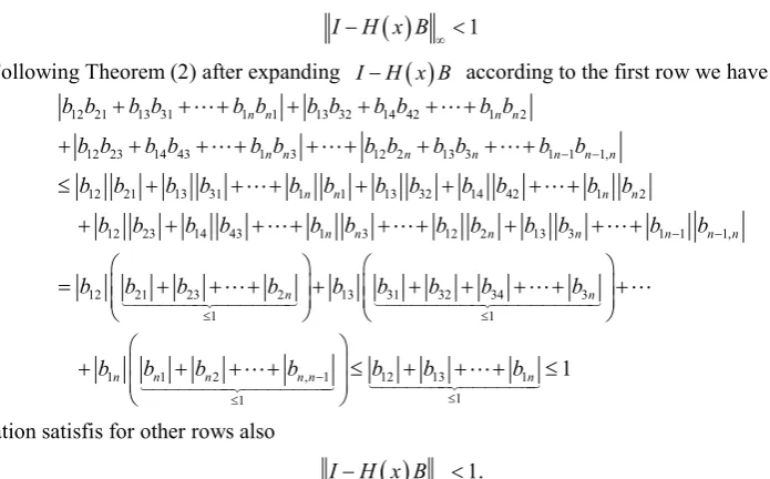
Proof: Following Theorem (2) after expanding I H x B−

( )

according to the first row we have

1 1 1 1 1 1 1 1 1 1

1 1 1 1 1 1

1 1 1 1 1 1 1

1 1 1 1 1 1 1 1 1

1 1

1 1 12 1 2 13 1 3 1 1 1 1

1 1 1 1 1 1

1 1 12 1 2 13 1 3 1 1

1 1 1 1 1 1 1 1

1 1

0

k k k k k k k k k k

k k k k n k k n

k k k k k k k

k k k k k k k n k k n

k k

b b b b b b b b b b b b b b b b b

b b

− −

+ +

−

− + +

+ − + + − + + + − +

+ + − + + + − +

≤ + − + + − + + + −

+ + − + + + − +

=

(

)

1 1 1 1 1 1

1 1

1 1 1

2 1 1

1

12 13 1 1 1 1 1

1 12 13 1 1 1 1 1 1.

k k k k k k n

k k n

k k k n

b b b b

b b b b b

b b b b b b

− +

≤

− +

 

 ₊ _{+ +} ₊ _{+ +} 

 

 

+ − + − + + − + − + + −

≤ + − + − + + − + − + + − ≤

This relation satisfis for other rows also

( )

1.

I H x B− _∞ <

5) We propose H x

( )

= +I S m

( )

+R such that S m

( )

and R was explained in (21) and (20) respectively and show that

( )

1.

I H x B− <

Theorem 6. If A is diagonally dominated and B=  bi j, , where b is defined ini j, (17) then

( )

1

I H x B− _∞ < Proof: Similar to proof of Theorems (3) and (5).

(7)

( )

1.

I H x B− <

( )

1

I H x B− _∞ <

Proof: Following Theorem (2) after expanding I H x B−

( )

according to the first row we have

12 21 13 31 1 1 13 32 14 42 1 2

12 23 14 43 1 3 12 2 13 3 1 1 1,

12 21 13 31 1 1 13 32 14 42 1 2

12 23 14 43 1 3 12 2 13 3 1 1 1,

1

n n n n

n n n n n n n

n n n n

n n n n n n n

b b b b b b b b b b b b

b b b b b b b b b b b b

b

− −

+ + + + + + +

+ + + + + + + + +

≤ + + + + + + +

+ + + + + + + + +

=

2 21 23 2 13 31 32 34 3

1 1

1 1 2 , 1 12 13 1

1 1

1

n n

n n n n n n

b b b b b b b b

b b b b b b b

≤ ≤

−

≤ ≤

   

+ + + + + + + + +

   

   

 

 

+ + + + ≤ + + + ≤

 

 

This relation satisfis for other rows also

( )

1.

I H x B− _∞ <

7) We propose H x

( )

= − +I U R such that U is the strictly upper triangular part of A and R was explained in (20) and show that

( )

1.

I H x B− <

( )

1

I H x B− _∞ <

Proof: Similar to proof of Theorems (3) and (7).

Now in the next section we apply H x

( )

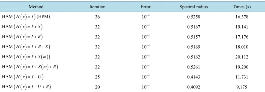
for solving numerical examples.

3. Numerical Results

In this section, we present some numerical examples to apply HAM and HPM methods for solving linear system. We used of Matlab 2013 for numerical results.

Example 1. Consider the linear system Ax b= , that

4 1 1

1 6 2 ,

0 1 3

A

−

 

 

= −_ _

 − 

 

7 9 5

b

    =      

and the exact solution is

1 2 1

x

    =    −  

[image:7.595.131.479.127.343.2]

.

Table 1 shows the iteration number,error,spectral radius of iteration matrix and computation time.

According to Table 1 we obtain the desirable result for solving this system by seven iterations with HAM and

( )

H x = − +I U R while by HPM method we used of fourteen iteration.

In this example the matrices S and S m

( )

are same and the results are same too.

Example 2. In this example we apply HAM method for solving the linear system Ax b=

(8)

[image:8.595.89.539.100.257.2]

Table 1. Camparision between HPM and HAM for 3 × 3 system.

Method Iteration Error Spectral radius Times (s)

HAM

(

H x( )=I

)

(HPM) 14 10−5 _0.4004 _0.013

HAM

(

H x( )= +I S

)

₁₁ ₁₀−5 _0.3057 _0.010

HAM

(

H x( )= +I R

)

9 10−5 _0.2168 _0.010

HAM

(

H x( )= + +I R S

)

₈ ₁₀−5 _0.1806 _0.014

HAM

(

H x( )= +I S m( )

)

11 10−5 _0.2918 _0.010

HAM

(

H x( )= +I S m( )+R

)

₈ ₁₀−5 _0.1806 _0.014

HAM

(

H x( )= −I U

)

8 10−5 _0.2918 _0.011

HAM

(

H x( )= − +I U R

)

₇ ₁₀−5 _0.1667 _0.011

Table 2. Camparision between HPM and HAM for 1000 × 1000 system.

Method Iteration Error Spectral radius Times (s)

HAM

(

H x( )=I

)

(HPM) 36 10−4 _0.5258 _16.378

HAM

(

H x( )= +I S

)

₃₂ ₁₀−4 _0.5167 _19.141

HAM

(

H x( )= +I R

)

32 10−4 _0.5157 _17.176

HAM

(

H x( )= + +I R S

)

₃₂ ₁₀−4 _0.5169 _18.010

HAM

(

H x( )= +I S m( )

)

32 10−4 _0.5162 _20.112

HAM

(

H x( )= +I S m( )+R

)

₃₂ ₁₀−4 _0.5261 _19.200

HAM

(

H x( )= −I U

)

25 10−4 _0.4143 _11.731

HAM

(

H x( )= − +I U R

)

₂₀ ₁₀−4 _0.4092 _9.175

4. Conclusion

From the numerical results, we have seen that the HAM method with different H x

( )

produces a spectral ra-dius smaller than the HPM and with the less iteration we obtain the desirable result.

Acknowledgements

We thank Islamic Azad University for support researcher plan entitled: “Combination of Iterative methods and semi analytic methods for solving linear systems” and the Editor and the referee for their comments.

References

[1] Nazari, A.M. and Zia Borujeni, S. (2012) A Modified Precondition in the Gauss-Seidel Method. Advances in Linear Algebra & Matrix Theory, 1, 31-37. http://dx.doi.org/10.4236/alamt.2012.23005

[2] Keramati, B. (2009) An Approach to the Solution of Linear System of Equations by He’s Homotopy Perturbation Me-thod. Chaos, Solitons and Fractals, 41, 152-156. http://dx.doi.org/10.1016/j.chaos.2007.11.020

[3] Liu, H.K. (2011) Application of Homotopy Perturbation Methods for Solving Systems of Linear Equations. Applied Mathematics and Computation, 217, 5259-5264. http://dx.doi.org/10.1016/j.amc.2010.11.024

[4] Liao, S.J. (1992) The Proposed Homotopy Analysis Technique for the Solution of Nonlinear Problems. Ph.D. Thesis, Shanghai Jiao Tong University, Shanghai.

[5] Morimoto, M., Harada, K., Sakakihara, M. and Sawami, H. (2004) The Gauss-Seidel Iterative Method with the Pre-conditioning Matrix.

(

I S S+ + m

)

. Japan Journal of Industrial and Applied Mathematics, 21, 25-34.

[image:8.595.88.538.283.439.2]

(9)

[6] Niki, H., Kohno, T. and Morimoto, M. (2008) The Preconditioned Gauss-Seidel Method Faster than the SOR Method.

Journal of Computational and Applied Mathematics, 218, 59-71. http://dx.doi.org/10.1016/j.cam.2007.07.002

[7] Niki, H., Kohno, T. and Abe, K. (2009) An Extended GS Method for Dense Linear System. Journal of Computational and Applied Mathematics, 231, 177-186. http://dx.doi.org/10.1016/j.cam.2009.02.005

[8] Yusefoglu, E. (2009) An Improvement to Homotopy Perturbation Method for Solving System of Linear Equations.

Computers & Mathematics with Applications, 58, 2231-2235. http://dx.doi.org/10.1016/j.camwa.2009.03.010

[9] Yuan, J.Y. and Zontini, D.D. (2012) Comparison Theorems of Preconditioned Gauss-Seidel Methods for M-Matrices.

Applied Mathematics and Computation, 219, 1947-1957. http://dx.doi.org/10.1016/j.amc.2012.08.037

[10] Gunawardena, A.D., Jain, S.K. and Snyder, L. (1991) Modified Iterative Method for Consistent Linear Systems. Linear Algebra and Its Applications, 154-156, 123-143. http://dx.doi.org/10.1016/0024-3795(91)90376-8

[11] Kohno, T. and Niki, H. (2009) A Note on the Preconditioner Pm=

(

I Sm+

)

. Journal of Computational and Applied Mathematics, 225, 316-319. http://dx.doi.org/10.1016/j.cam.2008.07.042

[12] He, J.H. (2003) Homotopy Perturbation Method: A New Non-Linear Analytical Technique. Applied Mathematics and Computation, 135, 73-79. http://dx.doi.org/10.1016/S0096-3003(01)00312-5

[13] Saad, Y. (2003) Iterative Methods for Sparse Linear Systems. SIAM Press, PHiladelphia. http://dx.doi.org/10.1137/1.9780898718003

[14] Liao, S.J. (2003) Beyond Perturbation: Introduction to the Homotopy Analysis Method. Chapman & Hall/CRC Press, Boca Raton. http://dx.doi.org/10.1201/9780203491164

[15] Liao, S.J. (2009) Notes on the Homotopy Analysis Method: Some Definitions and Theorems. Communications in Non-linear Science and Numerical Simulation, 14, 983-997. http://dx.doi.org/10.1016/j.cnsns.2008.04.013