Munich Personal RePEc Archive
A Pure-Jump Transaction-Level Price
Model Yielding Cointegration, Leverage,
and Nonsynchronous Trading Effects
Hurvich, Cliiford and Wang, Yi
Stern, NYU
4 December 2006
A Pure-Jump Transaction-Level Price Model Yielding
Cointegration, Leverage, and Nonsynchronous Trading Effects
Clifford M. Hurvich
∗Yi Wang
∗Abstract
We propose a new transaction-level bivariate log-price model, which yields fractional or standard cointegration. Most existing models for cointegration require the choice of a fixed sampling interval ∆t. By contrast, our proposed model is constructed at the transaction level, thus determining the properties of returns at all sampling frequencies. The two ingredients of our model are a Long Mem-ory Stochastic Duration process for the waiting times{τk}between trades, and a pair of stationary
noise processes ({ek}and{ηk}) which determine the jump sizes in the pure-jump log-price process.
The{ek}, assumed to bei.i.d.Gaussian, produce a Martingale component in log prices. We assume
that the microstructure noise {ηk} obeys a certain model with memory parameter dη ∈ (−1/2,0)
(fractional cointegration case) ordη=−1 (standard cointegration case). Our log-price model includes
feedback between the disturbances of the two log-price series. This feedback yields cointegration, in that there exists a linear combination of the two series that reduces the memory parameter from 1 to 1 +dη ∈(0.5,1)∪ {0}. Returns at sampling interval ∆t are asymptotically uncorrelated at any
fixed lag as ∆tincreases. We prove that the cointegrating parameter can be consistently estimated by the ordinary least-squares estimator, and obtain a lower bound on the rate of convergence. We propose transaction-level method-of-moments estimators of several of the other parameters in our model. We present a data analysis, which provides evidence of fractional cointegration. We then consider special cases and generalizations of our model, mostly in simulation studies, to argue that the suitably-modified model is able to capture a variety of additional properties and stylized facts, including leverage, portfolio return autocorrelation due to nonsynchronous trading, Granger causal-ity, and volatility feedback. The ability of the model to capture these effects stems in most cases from the fact that the model treats the (stochastic) intertrade durations in a fully endogenous way.
KEYWORDS: Tick Time; Long Memory Stochastic Duration; Information Share; Granger causality.
∗Stern School of Business, New York University.
I
Introduction
In this paper, we propose a transaction-level, pure-jump model for a bivariate price series, in which the intertrade durations are stochastic, and enter into the model in a fully endogenous way. The model is flexible, and able to capture a variety of stylized facts, including standard or fractional cointegration, persistence in durations, volatility clustering, leverage, and nonsynchronous trading effects. In this in-troduction, and indeed from here to Section VIII, we focus on cointegration, as this is the area in which we have so far been able to develop theoretical results on our model. Nevertheless, simulations show that a suitably-modified version of our basic model is able to produce the so-called leverage effect (i.e., negative autocorrelation between the current period’s return and the next period’s absolute return), as well as portfolio return autocorrelation due to nonsynchronous trading, Granger causality, and volatility feedback.
Cointegration has received considerable attention in Economics and Econometrics. Under both stan-dard and fractional cointegration, there is a contemporaneous linear combination of two or more time series which is less persistent than the individual series. Under standard cointegration, the memory pa-rameter is reduced from 1 to 0, while under fractional cointegration the level of reduction need not be an integer. Indeed, in the seminal paper of Engle and Granger (1987), both standard and fractional cointe-gration were allowed for, although the literature has developed separately for the two cases. Important contributions to the representation, estimation and testing of standard cointegration models include Stock and Watson (1988), Johansen (1988, 1991), and Phillips (1991). Literature addressing the corresponding problems in fractional cointegration includes Dueker and Startz (1998), Marinucci and Robinson (2001), Robinson and Marinucci (2001), Robinson and Yajima (2002), Robinson and Hualde (2003), Velasco (2003), Velasco and Marmol (2004), Chen and Hurvich (2003a, 2003b, 2006).
nature of observed asset-price processes.
Before describing the cointegration aspects of our model, we provide some background on transaction-level modeling. Currently, a wealth of transaction-transaction-level price data is available, and for such data the (observed) price remains constant between transactions. If there is a diffusion component underlying the price, it is not directly observable. Pure-jump models for prices thus provide a potentially appealing alternative to diffusion-type models. The compound Poisson process proposed in Press (1967) is a pure-jump model for the logarithmic price series, under which innovations to the log price are i.i.d., and these innovations are introduced at random time points, determined by a Poisson process. The model was generalized by Oomen (2006), who introduced an additional innovation term to capture market microstructure.
An informative and directly-observable quantity in transaction-level data is the durations{τk}between transactions. A seminal paper focusing on durations and, to some extent, on the induced price process, is Engle and Russell (1998). They documented a key empirical fact, i.e., that durations are strongly autocorrelated, quite unlike the i.i.d. exponential duration process implied by a Poisson transaction process, and they proposed the Autoregressive Conditional Duration (ACD) model, which is closely related to the GARCH model of Bollerslev (1986). Deo, Hsieh and Hurvich (2006) presented empirical evidence that durations, as well as transaction counts, squared returns and realized volatility have long memory, and introduced the Long Memory Stochastic Duration (LMSD) model, which is closely related to the Long Memory Stochastic Volatility model of Breidt, Crato and de Lima (1998) and Harvey (1998). The LMSD model isτk =ehkǫk where {hk} is a Gaussian long-memory series with memory parameter
dτ ∈ (0,1/2), the {ǫk} are i.i.d.positive random variables with mean 1, and {hk}, {ǫk} are mutually independent.
It was shown in Deo, Hurvich, Soulier and Wang (2006) that long memory in durations propagates to long memory in the counting processN(t), whereN(t) counts the number of transactions in the time interval (0, t]. In particular, if the durations are generated by an LMSD model with memory parameter
that varN(t) ∼Ct2dτ+1 as t → ∞. This long-range count dependence then propagates to the realized
volatility, under the simple return model considered in Deo, Hurvich, Soulier and Wang (2006).
In order to reflect the persistence in durations, we will assume in this paper that durations are generated by an LMSD model with memory parameter dτ ∈ (0,1/2). Thus, the resulting counting processN(t) will have long-range count dependence with the same memory parameter,dτ.
In this paper, we propose a pure-jump model for a bivariate log-price series such that any discretiza-tion of the process to an equally-spaced sampling grid with sampling interval ∆t produces fractional or standard cointegration,i.e., there exists a contemporaneous linear combination of the two log-price series which has a smaller memory parameter than the two individual series. A key ingredient in our model is a microstructure noise contribution{ηk} to the log prices. In the fractional cointegration case, this noise series obeys a fractional Gaussian noise model, with a corresponding memory parameterdη∈(−1/2,0), while in the standard cointegration case{ηk}is the difference of a white noise, and has memory parameter
dη = −1. In both cases, the reduction of the memory parameter is −dη. Due to the presence of the microstructure noise term, the discretized log-price series are not Martingales, and the corresponding re-turn series are not linear in either ani.i.d.sequence, a Martingale-difference sequence, or a strong-mixing sequence. This is in sharp contrast to existing discrete-time models for cointegration, most of which assume at least that the series has a linear representation with respect to a strong-mixing sequence.
The discretely-sampled returns (i.e., the increments in the log-price series) in our model are not Mar-tingale differences, due to the microstructure noise term. Instead, for small values of ∆tthey may exhibit noticeable autocorrelations, as observed also in actual returns over short time intervals. Nevertheless, the returns behave asymptotically like Martingale differences as the sampling interval ∆tis increased, in the sense that the lag-k autocorrelation tends to zero as ∆t tends to∞ for any fixedk. Again, this is consistent with the near-uncorrelatedness observed in actual returns measured over long time intervals.
thereby establishing the existence of cointegration in our model.
In order to derive the results described above, we will make use of the general theory of point processes, and we will also rely heavily on the theory developed in Deo, Hurvich, Soulier and Wang (2006) for the counting processN(t) induced by LMSD durations.
In Section II, we exhibit our pure-jump model for the bivariate log-price series. Since the two series need not have all of their transactions at the same time points (due to nonsynchronous trading), it is not possible to induce cointegration in the traditional way,i.e., by directly imposing in clock time an additive common component for the two series, with a memory parameter equal to 1. Instead, the common component is induced indirectly, and incompletely, by means of a feedback mechanism in transaction time between current log-price disturbances of one asset and past log-price disturbances of the other. This feedback mechanism also induces certain end-effect terms, which we explicitly display and handle in our theoretical derivations using the theory of point processes.
In Section III, we present the properties of the log-price series implied by our model. In particular, we show that the log price behaves asymptotically like a Martingale astis increased, and the discretely-sampled returns behave asymptotically like Martingale differences as ∆t is increased. We also present a lemma on the microstructure component of the log-price series. We show that this component, which is a random sum of the microstructure noise, has memory parameter 1 +dη <1.
In Section IV, we establish that our model possesses cointegration, by showing that the cointegrating error has memory parameter 1 +dη. We present two theorems, for the fractional and standard cointe-gration cases respectively, using a different definition of the memory parameter of the cointegrating error for each case.
In Section V, we show that the ordinary least squares (OLS) estimator of the cointegrating parameter
θis consistent, and obtain a lower bound on its rate of convergence.
In Section VII, we propose a method of moments estimator of the error and mirostructure feedback coefficients and variances. The estimator is based on the observed tick-time returns.
In Section VIII, we present data analyses of prices of classified stocks from a single company, buy and sell prices of a single stock, and transaction prices of stocks of two companies in the same industry, all of which provide evidence of fractional cointegration. We also consider the information share, which can be estimated based on the method of moments estimators from Section VII.
In Section IX, we demonstrate, largely through simulations, that modified versions of our model can reproduce two additional important stylized facts: leverage, and portfolio return autocorrelation due to nonsynchronous trading. We also show that the original model yields volatility feedback, and a modified version of the model can yield Granger causality. We trace all of these clock-time properties to their tick-time source.
In Section X, we provide some remarks and discuss possible further generalizations of our model and related future work.
II
A Pure-Jump Model For Log Prices
Suppose that there are two assets, 1 and 2, and that each log price is affected by two types of disturbances when a transaction happens. These disturbances are the efficient price shocks{ei,k}and the microstruc-ture noise {ηi,k}, for Asset i = 1,2. We assume that the {ei,k} are i.i.d. N(0, σ2
i,e). The fractional
cointegration case corresponds todη ∈(−12,0). In this fractional case, we assume that for i= 1,2, the
{ηi,k}, which are mutually independent, obey a fractional Gaussian noise model, with common memory parameterdη, i.e.
ηi,k=BH(k+ 1)−BH(k) (1)
where BH(t) is fractional Brownian motion with memory parameter dη = H − 1 2 ∈ (−
1
2,0). In this case, we will denoteσ2
Samorodnitsky and Taqqu (1994). The reason we choose the fractional Gaussian noise model is that it leads to a very simple expression for the variance of a partial sum, which is useful in the proof of Lemma 1.
The standard cointegration case corresponds todη=−1, and here we assume thatηi,k=ξi,k−ξi,k−1, where{ξi,k}∞
k=1arei.i.d.(0, σi,ξ2 ) noise series, with the nonrandom initializationξi,0= 0,i= 1,2. In this case, var(ηi,k) =σ2
i,η= 2σ2i,ξ.
The normality assumption on the efficient price shocks{ei,k}is only used in Theorem 5. The normality assumption on the microstructure noise {ηi,k} in the fractional case may be relaxed by considering a Fractional Laplace Noise. See Kozubowski, Meerschaert and Podgorski (2006). Note that we do not assume normality of the{ηi,k}in the standard cointegration case.
We now describe the tick-time return interactions that yield cointegration in our model. We will assume that the m-th tick-time return of Asset 1 incorporates not only its own current disturbances
e1,m andη1,m, but also weighted versions of all intervening disturbances of Asset 2 that were originally
introduced between the (m−1)-th and m-th transactions of Asset 1. The weight for the efficient price shocks, denoted by θ, may be different from the weight for the microstructure noise, denoted by g21 (the impact from Asset 2 to Asset 1). We similarly define them-th tick-time return of Asset 2, but the weight for the efficient price shocks from Asset 1 to Asset 2 is (1/θ) and the corresponding weight for the microstructure noise is denoted byg12. The choice of the second impact coefficient (1/θ) is necessary for the two log-price series to be cointegrated.
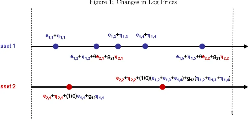
Figure 1 illustrates the mechanism by which tick-time returns are generated in our model. All dis-turbances originating from Asset 1 are colored in blue while all disdis-turbances originating from Asset 2 are colored in red. When the first transaction of Asset 1 happens, an efficient price shock e1,1 and a microstructure disturbance η1,1 are introduced. The first transaction of Asset 2 follows in clock time and since the first transaction of Asset 1 occurred before it, the return for this transaction is (e2,1+η2,1+ 1θe1,1+g12η1,1), i.e., the sum of the first efficient price shock of Asset 2, e2,1, the first
whose disturbances are e1,1 andη1,1, weighted by the corresponding feedback impact coefficients 1θ and g12. In the figure, both log-price processes evolve until timet. Notice that the third return of Asset 1 contains no feedback term from Asset 2 since there is no intervening transaction of Asset 2. The second return of Asset 2 includes its own current disturbances (e2,2, η2,2) as well as six weighted disturbances
[image:9.595.84.484.238.434.2](e1,2,e1,3,e1,4,η1,2,η1,3andη1,4) from Asset 1 since there are three intervening transactions of Asset 1.
Figure 1: Changes in Log Prices
At a given clock time t, most of the disturbances of Asset 1 are incorporated into the log price of Asset 2 and vice-versa. However, there is an end effect. The problem can be easily seen in the figure: since the fifth transaction of Asset 1 happened after the last transaction of Asset 2 before time t, the most recent Asset 1 disturbances e1,5 and η1,5 are not incorporated in the log price of Asset 2 at time
t. Eventually, at the next transaction of Asset 2, which will happen after time t, these two disturbances will be incorporated. But this end effect may be present at any given time t. We will handle this end effect explicitly in all derivations in the paper.
with memory parameters dτ1, dτ2 ∈(0,
1
2). The corresponding counting processes are denoted by Ni(t). Denote the clock time for thek-th transaction of Asseti byti,k. We also assume that{τ1,k} and{τ2,k}
are mutually independent and also independent of all disturbance series{e1,k},{e2,k},{η1,k}and{η2,k},
which implies thatN1(·) andN2(·) are mutually independent and independent of all disturbance series. Finally, all disturbance series are assumed to be mutually independent.
Our model for the log prices is then given for all non-negative real tby
logP1,t = NX1(t)
k=1
(e1,k+η1,k) +
N2(t1,N1 (t))
X
k=1
(θe2,k+g21η2,k) (2)
logP2,t = NX2(t)
k=1
(e2,k+η2,k) +
N1(t2,N2 (t))
X
k=1 (1
θe1,k+g12η1,k) .
Note that (2) implies that logP1,0 = logP2,0 = 0, the same standardization used in Stock and Watson (1988) and elsewhere.
The quantity N2(t1,N1(t)) represents the total number of transactions of Asset 2 occurring up to
the time (t1,N1(t)) of the most recent transaction of Asset 1. An analogous interpretation holds for the
quantityN1(t2,N2(t)).
To exhibit the various components of our model, we rewrite (2) as
logP1,t=
³NX1(t)
k=1
e1,k+ NX2(t)
k=1
θe2,k
| {z }
common component
´
+³
NX1(t)
k=1
η1,k+ NX2(t)
k=1
g21η2,k
| {z }
microstructure component
´ −
NX2(t)
k=N2(t1,N1 (t))+1
(θe2,k+g21η2,k)
| {z }
end effect
(3)
logP2,t=
³NX1(t)
k=1 1
θe1,k+ NX2(t)
k=1
e2,k
| {z }
common component
´
+³
NX1(t)
k=1
g12η1,k+ NX2(t)
k=1
η2,k
| {z }
microstructure component
´ −
NX1(t)
k=N1(t2,N2 (t))+1
(1
θe1,k+g12η1,k)
| {z }
end effect
.
Since both logP1,t and logP2,t areI(1) (see Theorem 1) and the linear combination logP1,t−θlogP2,t
isI(1 +dη) (by Theorems 3 and 4), the log-price series are cointegrated.
From (2) it can be seen that our model for the log price series can be represented in terms of subor-dinated Brownian motions and fractional Brownian motions, in the spirit of Clark (1973). For example, whenH ∈(0,1/2), logP1,tcan be written (up to a constant term) as
n
B1
³
N1(t)´+θB2
³
N2(t1,N1(t))
´o
+nB1,H
³
N1(t+ 1)´+g21B2,H
³
N2(t1,N1(t)+ 1)
´o
whereB1andB2are mutually independent Brownian motions, independent of the mutually independent fractional Brownian motionsB1,H and B2,H. The arguments forB1,H andB2,H would betrather than t+ 1, and the constant would be zero, if we had defined fractional Gaussian noise as the increment of a fractional Brownian motion at timesk−1 andkrather than the standardk,k+ 1. Here, the directing processes are the non-decreasing processesN1(t) andN2(t1,N1(t)), yielding a pure-jump price process.
Frijns and Schotman (2006) considered a mechanism for generating quotes in tick time which is similar to the mechanism we describe in Figure 1. However, they condition on durations, whereas we endogenize them in our model (2). Furthermore, their model implies standard cointegration, with cointegrating parameter that is known to be 1, and a single efficient shock component.
III
Long-Term Martingale-Type Properties Of the Log Prices
Define λ = 1/E0(τk), where E0 denotes expectation under the Palm distribution, i.e., the stationary distribution of{τk}. Note that λis a positive finite constant.
From (3) it can be seen that the microstructure components of the log price are random sums of the microstructure noise. The following lemma shows that such random sums have memory parameter 1 +dη<1, wheredη is the memory parameter of the microstructure noise.
Lemma 1 For durations {τk} generated by an LMSD model with memory parameterdτ ∈(0,1
fractional Gaussian noise series{ηk}with memory parameterdη=H−1 2 ∈(−
1
2,0), which is independent
of {τk},
var(
N(t)
X
k=1
ηk)∼(σ2λ2dη+1)t2dη+1
ast→ ∞, whereσ2= var[BH(1)]in Equation (1).
The following two theorems show that the log-price series in Model (2) have asymptotic variances that scale like t as t→ ∞, as would happen for a Martingale, and that their discretized differences are asymptotically uncorrelated as the discretization interval increases, as would happen for a Martingale difference series.
Define λ1= 1/E0(τ1,k) andλ2= 1/E0(τ2,k).
Theorem 1 For the log-price series in Model (2),
var(logPi,t)∼Cit, i= 1,2
ast→ ∞, whereC1= (σ12,eλ1+θ2σ22,eλ2)andC2= (σ22,eλ2+θ12σ21,eλ1).
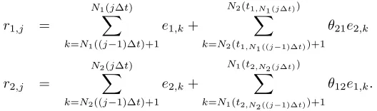
For a given sampling interval (equally-spaced clock-time period) ∆t, the returns for Asset 1 and 2 corresponding to Model (2) are
r1,j =
N1X(j∆t)
k=N1((j−1)∆t)+1
(e1,k+η1,k) +
N2(t1,N1 (j∆t))
X
k=N2(t1,N1 ((j−1)∆t))+1
(θe2,k+g21η2,k) (4)
r2,j =
N2(j∆t)
X
k=N2((j−1)∆t)+1
(e2,k+η2,k) +
N1(t2,N2 (j∆t))
X
k=N1(t2,N2 ((j−1)∆t))+1
(1
θe1,k+g12η1,k) .
Theorem 2 For any fixed integer k >0, the lag-k autocorrelation of {ri,j}∞j=1, i = 1,2, tends to 0 as
IV
Properties of the Cointegrating Error
We show that Model (2) implies a cointegrating relationship between the two series, treating the fractional and standard cointegration cases separately.
Theorem 3 Under Model (2) with dη ∈ (−1/2,0), the memory parameter of the linear combination
(logP1,t−θlogP2,t)is 1 +dη<1, that is,
var(logP1,t−θlogP2,t)∼C t2dη+1
ast→ ∞, whereC >0. Thus,logP1,t andlogP2,t are fractionally cointegrated.
Next, we investigate the standard cointegration case. It is important to note that, unlike in Theorem 3, where we measure the strength of cointegration using the asymptotic behavior of the variance of the cointegrating errors var(logP1,t−θlogP2,t), we need a different measure here since logP1,t−θlogP2,t
is stationary and its variance is constant for allt. Instead, we consider the asymptotic covariance of the cointegrating errors
cov(logP1,t−θlogP2,t,logP1,t+j−θlogP2,t+j)
asj→ ∞. We taketandj here to be positive integers,i.e., we sample the log-price series using ∆t= 1, without loss of generality.
We say that a sequence{aj}hasnearly-exponential decay ifaj/j−α→0 for allα >0 asj→ ∞. We
say that a stationary time series hasshort memory if its autocovariances have nearly-exponential decay.
Theorem 4 Under Model (2), with dη = −1, the cointegrating error (logP1,t −θlogP2,t) has short
V
Least-Squares Estimation of the Cointegrating Parameter
Assume that the log-price series are observed at integer multiples of ∆t. The proposed model (2) becomes
logP1,j =
N1X(j∆t)
k=1
(e1,k+η1,k) +
N2(t1,N1(j∆t))
X
k=1
(θe2,k+g21η2,k) (5)
logP2,j =
N2X(j∆t)
k=1
(e2,k+η2,k) +
N1(t2,N2(j∆t))
X
k=1 (1
θe1,k+g12η1,k) .
We show that the cointegrating parameterθcan be consistently estimated by OLS regression.
Theorem 5 For the discretely-sampled log-price series in (5), the cointegrating parameterθcan be
con-sistently estimated by θˆ, the ordinary least squares estimator obtained by regressing {logP1,j}nj=1 on
{logP2,j}nj=1 without intercept. For all δ >0,
n−dη−δ(ˆθ−θ)→p 0, asn→ ∞,
The rate of convergence of ˆθ improves asdη decreases. In the standard cointegration case dη =−1, the rate is arbitrarily close ton.
VI
Simulations on OLS Estimation of the Cointegrating
Param-eter
We study the performance of ˆθ in a simulation study carried out as follows.
First, we simulate two mutually independent duration process {τi,k}, i = 1,2, for Asset i. Each duration process follows the Long Memory Stochastic Duration (LM SD) model,
τi,k=ehi,kǫi,k
where the{ǫi,k}arei.i.d.positive random variables with all moments finite, and the{hi,k}are a Gaussian long-memory series with common memory parameterdτ ∈(0,1/2). Here, we assume that the{ǫi,k}follow a Weibull distribution with shape parameterκ= 1 and scale parameter ˜λ= 1, so thatE(ǫi,k) = 1. The
{hi,k} are simulated from a Gaussian ARFIMA(0,dτ, 0) model with unit innovation variance.
Using the simulated durations{τi,k},i= 1,2, we obtain the corresponding counting processes{Ni(t)}, usingti,1= Uniform[0, τi,1]. This ensures that the counting processes are stationary.
Next, we generate mutually independent disturbance series {e1,k},{e2,k},{η1,k} and {η1,k}. Here,
{ei,k}, i= 1,2,arei.i.d. N(0,1). Whendη ∈(−12,0), the{ηi,k}are given by fractional Gaussian noise as defined in (1) with σ2
1,η =σ22,η = 1, simulated using the algorithm on page 218 of Beran (1994). When dη = −1, {ηi,k} are simulated as the differences of two independent i.i.d.zero-mean standard normal series{ξi,k}.
We then construct the log-price series{logPi,j}n
j=1, i= 1,2 from (2), using a fixed sampling interval ∆t. The estimated cointegrating parameter ˆθ is obtained by regressing{logP1,j}jn=1on{logP2,j}nj=1.
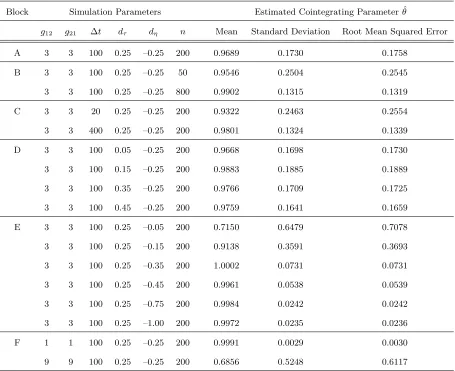
Table 1: Simulation Results on OLS Estimation of the Cointegrating Parameter
Block Simulation Parameters Estimated Cointegrating Parameter ˆθ
g12 g21 ∆t dτ dη n Mean Standard Deviation Root Mean Squared Error
A 3 3 100 0.25 –0.25 200 0.9689 0.1730 0.1758
B 3 3 100 0.25 –0.25 50 0.9546 0.2504 0.2545
3 3 100 0.25 –0.25 800 0.9902 0.1315 0.1319
C 3 3 20 0.25 –0.25 200 0.9322 0.2463 0.2554
3 3 400 0.25 –0.25 200 0.9801 0.1324 0.1339
D 3 3 100 0.05 –0.25 200 0.9668 0.1698 0.1730
3 3 100 0.15 –0.25 200 0.9883 0.1885 0.1889
3 3 100 0.35 –0.25 200 0.9766 0.1709 0.1725
3 3 100 0.45 –0.25 200 0.9759 0.1641 0.1659
E 3 3 100 0.25 –0.05 200 0.7150 0.6479 0.7078
3 3 100 0.25 –0.15 200 0.9138 0.3591 0.3693
3 3 100 0.25 –0.35 200 1.0002 0.0731 0.0731
3 3 100 0.25 –0.45 200 0.9961 0.0538 0.0539
3 3 100 0.25 –0.75 200 0.9984 0.0242 0.0242
3 3 100 0.25 –1.00 200 0.9972 0.0235 0.0236
F 1 1 100 0.25 –0.25 200 0.9991 0.0029 0.0030
9 9 100 0.25 –0.25 200 0.6856 0.5248 0.6117
More interestingly, the memory parameter of the duration process dτ has no discernible impact on the performance of ˆθ (See Blocks A and D). This is in agreement with the theoretical derivation for Theorem 5, in which dτ plays no role. On the other hand, the variance of ˆθ decreases sharply as the memory parameter of the microstructure noisedη decreases (see Blocks A and E). This is consistent with the results in Theorem 5, though the case dη = −0.75 is not covered by the theorem. (In this case, the microstructure noise{ηi,k}, i= 1,2 were simulated as the difference of the corresponding fractional Gaussian noise with memory parameterdη+ 1 = 0.25.)
VII
Method of Moments Parameter Estimation
We propose a simple (though clearly inefficient) transaction-level parameter estimation procedure for model (2) using the method of moments.
Consider Figure 1. The returns for the first, the third and the fourth transactions of Asset 1 have a simple structure, consisting of the sum of the current Asset 1 efficient and microstructure dusturbances, since for these transactions there was no intervening Asset 2 transaction. In general, we define a Type I transaction of Asset 1 as any Asset 1 transaction with no intervening Asset 2 transaction. Since {e1,k}
and{η1,k}are assumed to be mutually independent, the corresponding return variance for Type I Asset
1 transaction isσ2
1,e+σ21,η.
Consider the third and the fourth transactions of Asset 1 in Figure 1. This is a pair of adjacent Type I transactions. Since{e1,k} are assumed to bei.i.d., the covariance of the returns of such a pair is equal
to the lag-1 autocovariance of the microstructure noise series{η1,k}, given by
f(σ2i,η, dη) =
(22dη−1)σ2
i,η, dη∈(−12,0)
(22dη+2−1
23
2dη+1−7
2)σ 2
i,η, dη∈(−1,−12)
−σ2
1,ξ=−12σ2i,η, dη=−1.
(6)
transaction. An example is the second and the fifth Asset 1 transaction in Figure 1. The corresponding return variance isσ2
1,e+σ21,η+θ2σ22,e+g221σ22,η.
We can define Type-I, adjacent pairs of Type-I and Type-II transactions of Asset 2 in a similar manner.
For both assets, we compute the sample variance of the Type-I and Type-II transactions, as well as the sample covariance between adjacent pairs of Type-I transactions. The method-of-moments estimates ˆ
σ2
1,e, ˆσ12,η, ˆσ22,e σˆ22,η, ˆg12 and ˆg21 are given as the solutions to the following system, consisting of six equations.
c
var(Type I; Asseti) = ˆσi,e2 + ˆσi,η2 (i= 1,2) (7)
c
var(Type II; Asset 1) = ˆσ12,e+ ˆσ21,η+ ˆθ2σ22,e+ ˆg221ˆσ22,η
c
var(Type II; Asset 2) = ˆ1
θ2σˆ 2
1,e+ ˆg122 σˆ12,η+ ˆσ22,e+ ˆσ22,η
d
cov(Adjacent pairs of Type I; Asseti) = f(ˆσ2
i,η,dηˆ ) (i= 1,2)
where ˆθis an OLS estimator ofθas justified in Section V, ˆdη is obtained from the cointegrating residuals using the log-periodogram regression method, and the function f(ˆσ2
i,η,dηˆ ) is defined in (6). Note that
since bothg21 andg12appear as squares in the corresponding variances, we assume both to be positive.
A disadvantage of the method of moments is that the variance estimates ˆσ2
1,e, ˆσ12,η, ˆσ22,e σˆ22,η can be
negative. The same is true for ˆg2
[image:18.595.118.478.553.650.2]21 and ˆg122 . We set the corresponding estimates to be zero, if negative values are obtained in solving (7).
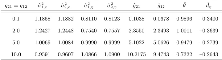
Table 2: Parameter Estimation using the Method of Moments
g21=g12 σˆ12,e σˆ
2 2,e σˆ
2
1,η ˆσ
2
2,η gˆ21 ˆg12 θˆ dˆη
0.1 1.1858 1.1882 0.8110 0.8123 0.1038 0.0678 0.9896 –0.3400
2.0 1.2427 1.2448 0.7540 0.7557 2.3550 2.3493 1.0011 –0.3639
5.0 1.0069 1.0084 0.9990 0.9999 5.1022 5.0626 0.9479 –0.2739
10.0 0.9591 0.9607 1.0866 1.0900 10.2175 9.4743 0.7322 –0.2643
estimators. The parameter values were dτ1 = dτ2 = 0.25, dη = −0.25, θ = 1, var(ei,k) = var(ηi,k) =
1,(i= 1,2). We variedg12 andg21, which we took to be equal. The{hi,k} were simulated as in Section VI. For each of 100 realizations, we simulated log prices in model (2) for a clock-time span of n∆t, with n = 100, ∆t = 50. The estimators ˆθ and ˆdη were constructed from the n = 100 clock-time log prices, and then these estimates were used together with the tick-time returns to yield the method of moments estimators. The estimator ˆdη was based on using the differenced cointegrating residuals in a log-periodogram regression with n0.5 frequencies, and then adding 1. The results, given in Table 2, are averages based on the 100 realizations. Asg12 is increased, all estimates except ˆθ become less biased.
VIII
Data Analysis
We analyze three empirical examples, corresponding to three different scenarios: prices of two classified stocks from a given company, buy and sell prices of a single stock, and prices of two different stocks within the same industry. In the first two situations, the cointegrating parameterθ would be expected to be 1, while in the third situation, there is no cleara priorivalue forθ.
Other possible scenarios that we do not pursue here include: (1) stock and option prices of a given company; (2) corporate bond prices at different maturities for a given company.
We obtained our data from the TAQ database of WRDS. We considered daily transactions between 9:30 AM to 4:00 PM. Overnight durations and returns are ignored, as implemented in, for example Hasbrouck (1995).
A
Prices of Classified Stocks from a Given Company
Corporation. The Class A and Class B common stock were combined as of the close of business on April 30, 2001. Class A stock has one vote per share while Class B stock has five votes per share.
We would expect the cointegrating parameter for the Class A and Class B log-prices to be close to 1. This is because Class A and B stocks have the same expected future cash flow. The only difference is the voting right, which only changes infrequently.
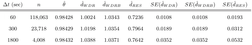
Our data spans the time period January 3, 2000 to April 30, 2001. Overall, there are 55,255 transac-tions of WDR and 10,689 transactransac-tions of WDRB. The average duratransac-tions are 131.78 and 653.16 seconds for WDR and WDRB, respectively.
[image:20.595.89.511.483.559.2]Based on the log-prices of WDR and WDRB observed every ∆t seconds, we computed the ordinary least squares estimates ˆθofθ, as well as log-periodogram regression estimates ˆdof the memory parameters for both log-price series as well as the cointegrating residuals (RES). The log-periodogram regression estimators were based on differences (with 1 subsequently added to the result), and used a number of frequencies equal to n0.7 for ˆdW DR and ˆdW DRB, and n0.6 for ˆdRES, chosen by visual inspection. The asymptotic estimated standard errors are also reported. The three choices of ∆tcorrespond to 1 minute, 5 minutes and 30 minutes. The results are reported in Table 3.
Table 3: Prices of Classified Stocks from a Given Company: WDR and WDRB
∆t(sec) n θˆ dˆW DR dˆW DRB dˆRES SE( ˆdW DR) SE( ˆdW DRB) SE( ˆdRES)
60 118,063 0.98428 1.0024 1.0343 0.7236 0.0108 0.0108 0.0193
300 23,718 0.98429 1.0198 1.0354 0.7964 0.0189 0.0189 0.0312
1800 4,008 0.98432 1.0388 1.0371 0.7642 0.0352 0.0352 0.0532
from (roughly) 1 to 0.75.
B
Buy and Sell Prices of a Single Stock
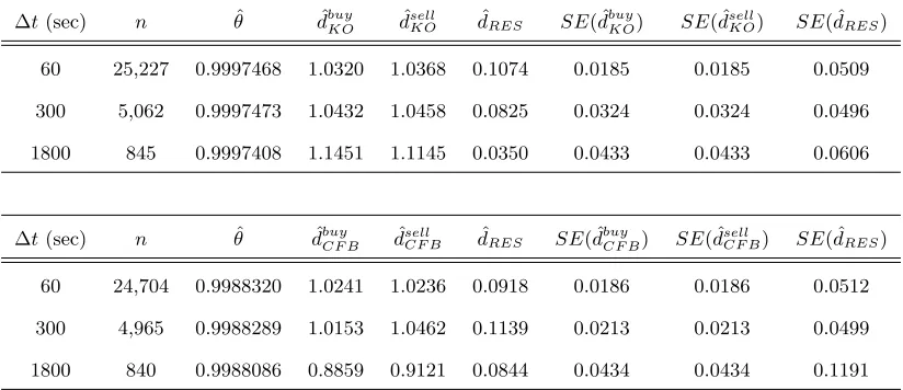
We consider buy and sell prices for a single stock. We analyze two different buy-sell data sets, one for a heavily-traded stock, Coca Cola (KO), and the other for a thinly-traded stock, Commercial Federal Bank (CFB). The data span the period from June 1, 2000 to August 31, 2000. Within this three-month period, there were 65 trading days (The market is closed on July 4, 2000) and 144,606 transactions of KO, 6,397 transactions of CFB.
We follow Lee and Ready (1991) to classify individual trades. If the transaction price is higher than the prior bid-ask midpoint, the current trade is labeled as a sell order. If the transaction price is lower, it is labeled as a buy order. If the transaction price is exactly the same as the prior bid-ask midpoint, the tick test (described in Lee and Ready 1991) is used to decide whether it should be classified as a buy or sell order.
[image:21.595.93.505.495.673.2]We study the buy and sell prices because they are closely related so that a strong cointegrating relationship is expected. Separating the buy and sell prices makes two series free of bid-ask bounce.
Table 4: Buy and Sell Prices of a Single Stock
∆t(sec) n θˆ dˆbuyKO dˆ
sell
KO dˆRES SE( ˆdbuyKO) SE( ˆd sell
KO) SE( ˆdRES)
60 25,227 0.9997468 1.0320 1.0368 0.1074 0.0185 0.0185 0.0509
300 5,062 0.9997473 1.0432 1.0458 0.0825 0.0324 0.0324 0.0496
1800 845 0.9997408 1.1451 1.1145 0.0350 0.0433 0.0433 0.0606
∆t(sec) n θˆ dˆbuy
CF B dˆ sell
CF B dˆRES SE( ˆdbuyCF B) SE( ˆdsellCF B) SE( ˆdRES)
60 24,704 0.9988320 1.0241 1.0236 0.0918 0.0186 0.0186 0.0512
300 4,965 0.9988289 1.0153 1.0462 0.1139 0.0213 0.0213 0.0499
The number of frequencies used in the log periodogram regressions vary from n0.5 ton0.8, chosen by visual inspection of log-log periodogram plots. As expected, the estimated cointegrating parameter is close to 1. Evidence of strong cointegration is found for both stocks. Furthermore, there is some evidence that the cointegration is fractional, and not standard.
C
Transaction Prices of Two Company Stocks within an Industry
We consider prices for the stocks of two companies within the same industry. Unlike in the previous examples, here there is noapriori value for the cointegrating parameterθ.
[image:22.595.101.493.380.458.2]The two companies we study are GM (GM) and Ford (F), within a one month period from June 1 to June 30, 2000. The results are given in Table 5. The cointegrating relationship between GM and Ford
Table 5: Transaction Prices of Two Company Stocks within an Industry
∆t(sec) n θˆ dˆGM dˆF dˆRES SE( ˆdGM) SE( ˆdF) SE( ˆdRES)
60 8,542 0.918506 0.9774 0.9848 0.8914 0.0172 0.0172 0.0270
300 1,715 0.918512 0.9659 0.9859 0.9468 0.0326 0.0326 0.0473
1800 286 0.918533 0.8968 1.1208 1.0338 0.0668 0.0668 0.1175
prices is much weaker than for the previous two examples, and because of this it is only significant for the smallest choice of the sampling interval ∆t.
D
Information Share
at timej on two different markets can be written as
logP1,j = logP1,0+
j
X
s=1
(ψ1˜e1,s+ψ2e˜2,s) +v1,j
logP2,j = logP2,0+
j
X
s=1
(ψ1˜e1,s+ψ2e˜2,s) +v2,j
where logP1,0 and logP2,0 are constants, (˜e1,s,˜e2,s)′ is a zero-mean vector of serially uncorrelated
dis-turbances with covariance matrix Ω, ψ = (ψ1, ψ2) are the weights for ˜e1,s,˜e2,s, and {(v1,j, v2,j)′} is a
zero-mean stationary bivariate time series. We regard ˜ei,s,(i= 1,2) as the innovation originating from the i-th market. The model in Hasbrouck (1995) is defined in clock time and is estimated using a one-second sampling interval. There, the information share of marketiis defined as
Si= ψ 2
iΩii ψΩψ′,
which is the proportional contribution from marketito the total random walk innovation variance. Only the random-walk component is used in constructing the information share since this is the only permanent component.
In our price model (3), we can also evaluate the information share, as described in words above. We consider two series, not necessarily the price of a given security on two different markets. For a given clock-time sampling interval ∆t, the information share of Asset 1, denoted byS1,C, is given by
S1,C =
var³ PN1(j∆t)
k=N1((j−1)∆t)+1e1,k
´
var³ PN1(j∆t)
k=N1((j−1)∆t)+1e1,k+θ
PN2(j∆t)
k=N2((j−1)∆t)+1e2,k
´ = λ1σ 2 1,e λ1σ12,e+θ2λ2σ22,e
.
Similarly, the information share of Asset 2 is given by
S2,C =
θ2λ 2σ22,e λ1σ12,e+θ2λ2σ22,e
.
Note that only the common component in (3) is used to evaluate the information share, as was also done by Hasbrouck (1995).
In Hasbrouck (1995), since the model is built in clock time, the trading intensities λ1, λ2 do not appear explicitly in the information share formulas, but instead the impact of these intensities is reflected inψΩψ′. By constrast,λ
As λ1/λ2→ ∞, S1,C approaches one and S2,C approaches zero. This is consistent with the general
intuition: an actively-traded security should reveal more information than a thinly-traded one. Indeed, Hasbrouck (1995) found that, for the 30 Dow-Jones stocks, the preponderance of the price discovery takes place at the NYSE and the majority of the transactions occurred on the NYSE.
To estimate the information share, estimates for the trading intensitiesλ1,λ2, and the efficient inno-vation variancesσ2
1,e,σ22,e are needed. To estimateλi,(i= 1,2), we use the total number of transactions
divided by the total period of observation for asseti. We estimateσ2
1,eandσ22,eby the method of moments
as discussed in section VII. We estimateθ using OLS, with ∆t= 60 seconds.
We consider the information shares of the buy and sell prices of a single stock: Coca Cola (KO). A question of interest is whether buy trades contain more information and therefore are more important for the price discovery process than sell trades. The data spans a 65 trading-day period from June 1 to August 31, 2000. The tick-time stock prices are plotted in Figure 2.
[image:24.595.113.489.501.638.2]We estimate the information share for each of three clock-time periods. Period one is the entire three-month interval comprising 65 trading days. Period two spans 36 trading days in which the stock price rose by roughly 20%. Period three comprises 22 trading days in which the stock price dropped by approximately 20%. The results are given in Table 6.
Table 6: Information Shares of Buy and Sell Price of KO
Period Type # of trades λˆi(per day) ˆσ2i,e σˆ
2
i,η Sˆi,C
1: 06/01 – 08/31/2000 Buy 74,856 1151.63 5.38e-07 4.45e-08 0.5144
Sell 69,750 1073.08 5.46e-07 4.75e-08 0.4856
2: 06/07 – 07/27/2000 Buy 42,804 1189.00 6.96e-07 4.39e-08 0.5813
Sell 39,437 1095.47 5.44e-07 4.37e-08 0.4187
3: 08/02 – 08/31/2000 Buy 23,800 1081.82 3.15e-07 4.26e-08 0.4120
Sell 21,626 983.00 4.95e-07 6.74e-08 0.5880
and sells. For period two when the stock price increases dramatically, the buy trades possess much more information than sell trades. By contrast, during period three when price has a significant drop, the sell trades have more information.
Figure 2: KO Stock Price in June to August, 2000
IX
Modifications of the Model to Capture More Stylized Facts
A
Volatility Feedback
In Model (2) we have assumed that N1(·) and N2(·) are mutually independent. Thus, for any fixed sampling interval ∆t, the resulting series of counts,{∆N1,j}, {∆N2,j} are mutually independent, where
∆N1,j = N1(j∆t)−N1([j−1]∆t) and ∆N2,j = N2(j∆t)−N2([j−1]∆t). From Clark (1973) (see
also Deo, Hurvich, Soulier and Wang (2006)), it is known for univariate series that the autocorrelation properties of realized volatility are related to those of counts. Thus, it may appear that for the bivariate returns (4) corresponding to model (2), the realized volatilities of the two series should be mutually independent. However, inspection of (4) reveals that bothN1(·) andN2(·) appear in the equations for both return series, {r1,j} and {r2,j}. Therefore, there is reason to suspect that in fact the realized
volatilities for the two return series will be mutually dependent. For example, if in a given time period the durations of Asset 1 are shorter than average (yielding a large contribution to the realized volatility of Asset 1), then although this will have no effect on the durations of Asset 2 it will still tend to produce a large number of shocks in the Asset 2 return, due to the return feedback mechanism shown in Figure 1, leading to a large contribution to realized volatility for Asset 2 from this time period.
We performed a small simulation study to confirm the volatility feedback effect. The parameter values weredτ1 =dτ2 = 0.35, dη =−0.25, θ = 1, var(ei,k) = var(ηi,k) = 1,(i= 1,2). We variedg12 and g21
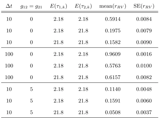
(which we took to be equal), to include or exclude the microstructure noise. We also varied the sampling frequency ∆tand the expected values of the durations of the two assets. The{hi,k}were simulated as in Section VI with unit innovation variance. The results, presented in Table 7, are based on 100 realizations of lengthn= 500. We denote byrRV the contemporaneous cross correlation of the realized volatilities of the two assets. Here, the realized volatilities were computed by summing the tick-time squared returns within each time period of width ∆t. This version of realized volatility was also considered in Andersen, Bollerslev, Frederiksen and Nielsen (2006).
It is seen from Table 7 that, as the average duration decreases or the sampling interval increases,rRV
Table 7: Simulation for the Volatility Feedback Effect
∆t g12=g21 E(τ1,k) E(τ2,k) mean(rRV) SE(rRV)
10 0 2.18 2.18 0.5914 0.0084
10 0 2.18 21.8 0.1975 0.0079
10 0 21.8 21.8 0.1582 0.0090
100 0 2.18 2.18 0.9609 0.0016
100 0 2.18 21.8 0.5763 0.0100
100 0 21.8 21.8 0.6157 0.0082
10 5 2.18 2.18 0.1140 0.0048
10 5 2.18 21.8 0.1591 0.0060
10 5 21.8 21.8 0.0508 0.0037
B
Portfolio Return Autocorrelation Due to Nonsynchronous Trading
The problem of nonsynchronous trading was first pointed out by Fisher (1966) and the issue has played an important role in the subsequent finance literature. Nonsynchronous trading can adversely affect pa-rameter estimation in the market model, (see, e.g., Scholes and Williams 1977), as well as the estimation of the covariance matrix of the returns (Shanken 1987), and can partially explain the positive autocor-relation of portfolio returns (see, e.g., Atchison, Butler and Simonds 1987, Lo and Mackinlay 1990 a,b, Boudoukh, Richardson and Whitelaw 1994, Kadlec and Patterson 1999).
reverted to the even stronger assumption of Scholes and Williams (1977) that there is no nontrading. Nevertheless, in one important respect, the assumptions of Badoukh, Whitelaw and Richardson (1994) are general, since they allow for cross-sectional dependence of the returns, unlike Scholes and Williams (1977). Recently, Kadlec and Patterson (1999) used a simulation-based approach to assess portfolio autocorrelation due to nonsynchronous trading, in which they use the event times as observed in actual data. Still, Kedlac and Patterson (1999) do not fully endogenize the event times, since if one wanted to run another simulation in their framework, they would have to use the same set of event times.
Up to now, the nontrading mechanism has not been modeled truly endogenously. In this paper, we model the duration process of the price directly, thus endogenize the nontrading mechanism in the price process.
To gain a better picture of the nonsynchronous trading effect implied by our model, we ignore tem-porarily the microstructure noise. Also, since stock prices may not be cointegrated in general, we change the efficient shock feedback coefficients in Model (2), 1/θandθ, toθ12andθ21, respectively. The resulting return series become
r1,j =
N1X(j∆t)
k=N1((j−1)∆t)+1 e1,k+
N2(t1,N1(j∆t))
X
k=N2(t1,N1 ((j−1)∆t))+1
θ21e2,k (8)
r2,j =
N2X(j∆t)
k=N2((j−1)∆t)+1 e2,k+
N1(t2,N2(j∆t))
X
k=N1(t2,N2 ((j−1)∆t))+1 θ12e1,k.
Lemma 2 Consider a portfolio consisting ofs1 shares of Asset 1 ands2shares of Asset 2, where the
re-turns on the two assets are given by (8). Suppose thatθ12>0andθ21>0. Then the lag-1 autocorrelation
[image:28.595.167.431.421.499.2]of the portfolio return isO(∆t−1)as∆t→ ∞, and is positive for all values of∆t.
Table 8 presents simulated averages of the lag-1 autocorrelations of returns of Asset 1, Asset 2 and a portfolio consisting of one share of each asset, i.e., s1 =s2 = 1, based on 5000 realizations. We also present the minimum and maximum portfolio autocorrelations. The LMSD model implemented here is
τi,k = 10ehi,kǫi,k,(i = 1,2). We used n= 500, θ
12 =θ21 = 1, dτ1 =dτ2 = 0.45 but vary the sampling
Table 8: Simulated Lag-1 Autocorrelations to Show Nonsynchronous Trading Effects
∆t 10 50 200
Asset 1 mean –0.0018 –0.0014∗ –0.0017∗
Asset 2 mean –0.0010 –0.0017∗ –0.0014∗
Portfolio mean 0.1077∗∗∗ 0.0894∗∗∗ 0.0376∗∗∗
maximum 0.3039 0.3354 0.2369
minimum –0.0668 –0.1321 –0.1288
∗,∗∗and∗∗∗indicate two-tailed significance at level 5%, 1% and 0
.1%, respectively.
Individual asset returns do not show strong autocorrelation. Nevertheless, the portfolio return has significant positive autocorrelation for all sampling intervals ∆tconsidered. The mean autocorrelations range from 0.0376 to 0.1077. The maximum portfolio autocorrelation can be as high as 0.3354. As ∆t
increases, the portfolio autocorrelation decreases, consistent with the theory described above.
In this paper, we only have two assets. With more assets, it may be possible to obtain far more spurious autocorrelation in the portfolio due to nonsynchronous trading. Empirically, as discussed in Perry (1985), the portfolio lag-1 autocorrelation increases as the number of securities in the portfolio increases. The generalization of our model to the case ofN ≥3 assets is beyond the scope of the current paper, but will be the subject of future research.
C
Granger Causality
Consider the return model (8). Suppose that θ12 6= 0 but θ21 = 0. Then the clock-time returns for Asset 2, {r2,j}, will contain contributions from both tick-time shock series {e1,k} and {e2,k}, whereas
the returns from Asset 1 will only contain contributions from{e1,k}. Roughly speaking, new information
directionality. If, for example, we were to fit a (misspecified) bivariateAR(1) model to the return data, we might expect to find that{r1,j}Granger-causes{r2,j}but that{r2,j}does not Granger-cause{r1,j}.
To get a clearer idea of why this might happen, note that although the individual return series are serially uncorrelated, there is a cross-correlation between the two returns when Asset 1 leads Asset 2 but not when Asset 2 leads Asset 1. This follows from the proof of Lemma 2 and is also in accord with intuition. For example, if Asset 1 was the last asset to trade in time period j−1 then the corresponding Asset 1 shock will be incorporated into the Asset 2 return at a time period after j−1. However, no Asset 2 shock will ever be incorporated into the Asset 1 return.
To study the causality properties of Model (8) under various restrictions, we simulated returns from the model using the same parameter values as in Table 7 (unless otherwise indicated). For each pair of simulated returns, we ran two OLS regressions: (1) Current returns of Asset 1 on lagged returns of both assets; (2) Current returns of Asset 2 on lagged returns of both assets. Table 9 reports means (over the 100 replications), and corresponding standard errors, for the estimated coefficient of lagged returns of Asset 2 in regression (1), and lagged returns of Asset 1 in regression (2). Denoting the population versions of these two regression coefficients asπ12 andπ21, it is seen that there is strong evidence that
[image:30.595.113.486.544.659.2]π21>0 but we cannot reject the hypothesis thatπ12= 0. Thus, at least in the context of the misspecified bivariate AR(1) model, it seems that the above-conjectured patterns in Granger causality indeed hold. The strength ofπ21diminishes as ∆tincreases, since it is the nonsynchronous trading effect that induces the causality.
Table 9: Simulation Results for Granger Causality
∆t θ12 θ21 mean(ˆπ12) SE(ˆπ12) t-stat(ˆπ12) mean(ˆπ21) SE(ˆπ21) t-stat(ˆπ21)
10 10 0 –0.0001 0.0005 –0.20 4.6588 0.0565 82.40
20 10 0 –0.0006 0.0007 –0.84 4.8621 0.0728 66.82
50 10 0 0.0011 0.0010 1.14 4.6951 0.0911 51.56
20 5 0 –0.0013 0.0014 –0.90 2.2726 0.0378 60.14
D
The Leverage Effect
The leverage effect is a negative correlation between the current return and future volatility (say, absolute return). We obtain a leverage effect in clock time by introducing a positive lagged cross-correlation between the current efficient shock ek and the next-transaction innovation (νk+1) to the log duration. The moving average representation of the long-memory component hi,k of τi,k in the LMSD model for durations can be written as hi,k = P∞j=0ψjνi,k−j where {ψj} are constants with P∞j=0ψj2 < ∞ and
{νi,k} is an i.i.d.Gaussian series with mean zero and variance σ2
νi. We will show using simulation that
a positive correlation betweenνi,k+1 andei,k in transaction time induces a clock-time leverage effect for the Assetireturn.
Specifically, we assume that ei,k = σi,e(φiνi,k+1+wi,k)/
q
φ2
iσ2νi+ 1, where ψi (i = 1,2) are
con-stants, and the {wi,k} are i.i.d. standard normal, independent of {νi,k}. Thus, corr(ei,k, νi,k+1) =
φiσνi/ q
φ2
iσν2i+ 1. As described in Section VI, the Asset i durations {τi,k} follow an LMSD model,
τi,k =ehi,kǫi,k, where {hi,k} follow an ARFIMA(0,dτ
i, 0) model and{ǫi,k}, independent of {hi,k}, are
i.i.d.Weibull with shape parameterκiand scale parameter ˜λisuch thatE(ǫi,k) = 1. A simple calculation yields
corr(ei,k, τi,k+1) = φiσ 2
νi q
φ2
iσ2νi+ 1
·r 1
˜
λ2
iΓ(1 +κ2i)e
σ2
νi
Γ(1−2dτi) Γ2 (1−dτi)
−1
.
The intuition for why this should produce a leverage effect is that if the current return shock is negative, this induces a below-average shockνk+1to the log duration, which then persists in the duration series to yield a sequence of below-average durations, i.e., frequent trading in clock time, and above-average volatility.
We verify using simulations that the correlation introduced above yields a leverage effect. For sim-plicity, we set the microstructure noise to zero. The resulting two-asset return model is given by (8). We simulatedn= 500 clock-time returns{ri,j}n
(2006). We also compared the portfolio return autocorrelations to those simulated under independence ofei,k andνi,k+1.
Note that corr(ri,j, ri,j+1) is the return lag-1 autocorrelation for Asseti= 1,2, while corr(|ri,j|, ri,j+1) and corr(|ri,j|, ri,j−1) measure the risk-premium effect (RP) and leverage effect (Lev), respectively. Other parameter values used in the simulation areθ= 1,dτ1 =dτ2 = 0.45,σi,e= 1, var(νi,k) =
Γ2(1−d
τ)
Γ(1−2dτ)so that
[image:32.595.95.508.289.444.2]var(hi,k) = 1 fori= 1,2,κi = ˜λi = 1,(i= 1,2). Results are based on 5000 realizations, and reported in Table 10.
Table 10: Risk Premium, Leverage, and Portfolio Autocorrelation from Simulations
Asset 1 Asset 2 Portfolio
∆t φi corr(ei,k, τi,k+1) RP Lev RP Lev Lag-1 Autocorr
10 0 0 –0.0006 0.0008 –0.0005 –0.0002 0.1077∗∗∗
5 0.23 –0.0059∗∗∗ –0.0924∗∗∗ –0.0062∗∗∗ –0.0916∗∗∗ 0.1279∗∗∗
50 0 0 –0.0005 0.0002 0.0002 –0.0004 0.0894∗∗∗
5 0.23 0.0018∗∗ –0.1178∗∗∗ 0.0011 –0.1169∗∗∗ 0.1038∗∗∗
200 0 0 –0.0008 0.0000 –0.0002 –0.0008 0.0376∗∗∗
5 0.23 0.0047∗∗∗ –0.1097∗∗∗ 0.0043∗∗∗ –0.1105∗∗∗ 0.0432∗∗∗
∗,∗∗and∗∗∗indicate two-tailed significance at level 5%, 1% and 0
.1%, respectively.
A positive correlation between {ei,k} and {νi,k+1} induces a significant leverage effect (with the predicted negative sign) for all values of ∆t. The magnitude of the leverage effect can be as large as 10%. On the other hand, the magnitude of the simulated risk-premium effect is always much smaller than that of the leverage effect: the corresponding ratio is no larger than 7%. Andersen, et. al. (2006) concluded from an analysis of 30 blue-chip stocks, there is evidence of a leverage effect, but no convincing evidence of a risk premium effect, so our model is consistent with their findings. The risk premium effect produced by our model, though small, has the interesting property that it is negative for short horizons, but becomes positive for long horizons.
In each case, the two-samplet-test of equal means for the lag-1 return autocorrelation with and without the leverage effect leads to rejection of the null hypothesis at the 0.1% level. The leverage effect can increase the portfolio return autocorrelation by as much as 2%, as found for ∆ = 10. In the Finance literature, it has been concluded that nonsynchronous trading can explain at most part of the portfolio return autocorrelation; see, for example, Lo and MacKinlay (1990 a,b). We feel that this question merits re-investigation, in the light of the model we have proposed in which durations are fully endogenized, and in the light of our current finding of interactions between the leverage effect and nonsynchronous trading effects.
X
Remarks and Suggestions for Future Work
Remark 1: Although we have assumed that the durations are generated by the LMSD model, the
theoretical results of Sections III, IV and V on cointegration continue to hold under the more general conditions given in Theorem 1 of Deo, Hurvich, Soulier and Wang (2006), which would allow, for example, the Autoregressive Conditional Duration model of Engle and Russell (1998).
Remark 2: In the fractional cointegration case, we have assumed that the memory parameter dη of
the microstructure noise components {ηi,k} (i = 1,2) lies in the range (−0.5,0). Two generalizations may be of interest. First is the case dη = 0, which implies that there is no cointegration, as would be the case for a factor model such as CAPM, see Sharpe (1964). Second is the case dη ∈ (−1,−1/2), which should presumably result in stronger fractional cointegration than we have allowed with our pre-vious restrictions. We have only a partial understanding of what would happen in this case. To obtain
we would get fractional cointegration in this case, but we are currently unable to establish the exact degree of cointegration; we can merely show that it is at least is strong as what would be obtained for
dη∈(−1/2,0). The OLS estimator ofθwould still be consistent, with a rate that is at least as fast as√n.
Remark 3: There is an important caveat regarding the Martingale property in the special case of
model (2) in which the microstructure noise components {η1,k} and{η2,k} are absent. For each series,
as long as the conditioning set involves only returns of the given series up to timet, the log price series (observed at discrete, equally spaced time intervals) is a Martingale. The Martingale property is lost, however, if the conditioning set is augmented to include returns on both assets up to timet. Because of the feedback effect in the model, and the nonsynchronous trading, recent information about Asset 1 can help to predict the Asset 2 return, even though the Asset 2 return is unpredictible based on its own past. Such a situation can occur in actual markets. For example, to predict the (real) return on the sale of a given home, it helps to know the returns on sales of similar homes that have taken place recently, though it may not help at all to know the past returns on sales of the given home, especially if it has not been sold for a long time.
Remark 4: In certain situations it might be useful to allow for different additive constants in the
model (2) for logP1,tand logP2,t. In particular, we could consider adding a positive constantCto logP1,t
and subtractingCfrom logP2,t(cf.Roll, 1984). This would have no effect on any of the theoretical results
on cointegration or the OLS estimation of the cointegrating parameter. In the example we considered in Section VIII of buy and sell prices of a given stock, the constantC could represent transaction costs. Note that it would still not necessarily be the case that logP1,t exceeds logP2,t, but such a constraint
is not needed here since the buy and sell markets trade nonsynchronously. The constant C would not be estimable by OLS (which would still be run without an intercept), but could be estimable from the cointegrating residuals if there is strong cointegration, withdη<−1/2.
Finally, we list a few possibilities for future work stemming from the current project.
asset allocation, pairs trading and index tracking in the current pure-jump context. So far, work has been done for option pricing based on pure-jump processes (Prigent, 2001) and dynamic asset allocation based on jump-diffusion processes (Liu, Longstaff and Pan, 2003), but these papers do not allow for cointegration. Another strand of literature has shown that, in a diffusion context, cointegration may have an impact on option pricing (Duan and Pliska, 2004), and on index tracking (Dunis and Ho, 2005; Alexander and Dimitriu, 2005), but these papers do not allow for a pure-jump process.
Other estimators of the cointegrating parameter could be considered, besides OLS. Though many such estimators have been proposed for both standard and fractional cointegration, none have yet been justified under a transaction-level model such as (2). Semiparametric estimators could be considered, since by the remark above the results of this paper do not require a parametric model for durations.
Generalizations of our model (2) could also be studied. For example, we could relax the assumptions that N1(·) and N2(·) are independent. For a related model, see Hsieh and Hurvich (2006). Finally, the possibility of more than two assets as well as deterministic linear trends should be considered.
References
[1] Alexander, C. (1999), Optimal Hedging Using Cointegration,Philosophical Transactions of the Royal Society A 357, 2039–2058.
[2] Alexander, C. and Dimitriu, A. (2005), Indexing, Cointegration and Equity Market Regimes, Inter-natiional Journal of Finance and Economics 10, 213–231.
[3] Andersen, T., Bollerslev, T., Frederiksen, P. and Nielsen M. (2006), Continuous-time Models, Realized Volatilities, and Testable Distributional Implications for Daily Stock Returns. Working Paper.
[5] Bollerslev. T. (1986), Generalized Autoregressive Conditional Heteroskedasticity,Journal of Econo-metrics 31, 307–327.
[6] Boudoukh, J., M. Richardson and R. Whitelaw (1994), A Tale of Three Schools: Insights on Autcor-relations of Short-Horizon Returns,Review of Financial Studies 7, 539–573.
[7] Breidt, F., Crato, N. and de Lima, P. (1998), The Detection and Estimation of Long Memory in Stochastic Volatility,Journal of Econometrics 83, 325–348.
[8] Chen, W. and Hurvich, C. (2003a), Estimating Fractional Cointegration in the Presence of Polynomial Trends,Journal of Econometrics 117, 95–121.
[9] Chen, W. and Hurvich, C. (2003b), Semiparametric Estimation of Multivariate Fractional Cointegra-tion,Journal of the American Statistical Association 98, 629–642.
[10] Chen, W. and Hurvich, C. (2006), Semiparametric Estimation of Fractional Cointegrating Subspaces, Forthcoming inAnnals of Statistics.
[11] Clark, P.K. (1973), A subordinated stochastic process model with finite variance for speculative prices,Econometrica 41, 135–155.
[12] Deo, R., Hsieh, M. and Hurvich, C. (2006), The Persistence of Memory: From Durations to Realized Volatility. Working Paper, Stern School of Business New York University.
[13] Deo, R., Hurvich, C., Soulier, P. and Wang Y. (2006), Conditions for the Propagation of Memory Parameter from Durations to Counts and Realized Volatility. Working Paper, Stern School of Business New York University.
[14] Duan, J.C. and Pliska, S. (2004), Option Valuation with Cointegrated Asset Prices, Journal of Economic Dynamics and Control 28, 727–754.
[16] Dunis, C.L. and Ho, R. (2005), Cointegration Portfolios of European Equities for Index Tracking and Market Neutral Strateries,Journal of Asset Management 6, 33-52.
[17] Engle, R. and Granger C.W.J. (1987), Co-integration and Error Correction: Representation, Esti-mation and Testing,Econometrica 66, 1127–1162.
[18] Engle, R. and Russell J. (1998), Autoregressive Conditional Duration: a New Model for Irregularly Spaced Transaction Data,Econometrica 66, 1127–1162.
[19] Fisher, L. (1966), Some New Stock Market Indices,Journal of Business 39, 191–225.
[20] Frijns, B. and Schotman, P. (2006), Price Discovery in Tick Time, Working Paper.
[21] Harvey, A.C. (1998), Long Memory in Stochastic Volatility,in: J. Knight, S. Satchell (Eds.), Fore-casting Volatility in Financial Markets, Butterworth-Heineman, Oxford, 307–320.
[22] Hasbrouck, J. (1995), One Security, Many Markets: Determining the Contributions to Price Discov-ery, Journal of Finance 50, 1175–1199.
[23] Hsieh, M. and Hurvich, C.M. (2006), Long Memory Models for Durations of Bivariate Series, Working Paper.
[24] Isserlis, L. (1918), On a Formula for the Product-Moment Coefficient of any Order of a Normal Frequency Distribution in any Number of Variables,Biometrika 12, 134–139.
[25] Johansen, S. (1988), Statistical Analysis of Cointegration Vectors, Journal of Economic Dynamics and Control 12, 231–254.
[26] Johansen, S. (1991), Estimation and Hypothesis Testing of Cointegration Vectors in Gaussian Vector Autoregressive Models,Econometrica 59, 1551–1580.
[27] Kadlec, G. and Patterson, D. (1999), A Transactions Data Analysis of Nonsynchronous Trading,
Revies of Financial Studies 12, 609–630.
[29] Liu, J., Longstaff, F. and Pan, J. (2003), Dynamic Asset Allocation with Event Risk, Journal of Finance 58, 231–259.
[30] Lee, C. and M. Ready (1991), Inferring Trade Direction from Intraday Data,Journal of Finance 46,
733–746.
[31] Lo, A. and A.C. MacKinlay (1990a), An Econometric Analysis of Nonsynchronous Trading,Journal of Econometrics 45, 181–211.
[32] Lo, A. and A.C. MacKinlay (1990b), When are Constrarian Profits Due to Stock Market Overreac-tion?,Revies of Financial Studies 3, 175–205.
[33] Marinucci, D. and Robinson, P.M. (2001), Semiparametric Fractional Cointegration Analysis. Fore-casting and empirical methods in finance and macroeconomics,Journal of Econometrics105, 225–247.
[34] Oomen, R.C.A., (2006), Properties of Realized Variance under Alternative Sampling Schemes, Jour-nal of Business and Economic Statistics 24, 219–237.
[35] Perry, P. (1985), Portfolio Serial Correlation and Nonsynchronous Trading,Journal of Financial and Quantitative Analysis 20, 517–523.
[36] Phillips, P.C.B. (1991), Optimal Inference in Cointegrated Systems,Econometrica 59, 283–306.
[37] Phillips, P.C.B. and Durlauf, S. (1986), Multiple Time Series Regression with Integrated Processes,
The Review of Economic Studies 53, 473–495.
[38] Press, S.J. (1967), A Compound Events Model for Security Prices,Journal of Business40, 317–335.
[39] Prigent, J-L. (2005), Option Pricing with a General Marked Point Process,Mathematics of Opera-tions Research 26, 50–66.
[40] Robinson, P.M. and Haulde, J. (2003), Cointegration in Fractional Systems with Unknown Integra-tion Orders,Econometrica 71, 1727–1766.
[42] Robinson, P.M. and Yajima, Y. (2002), Determination of cointegrating rank in fractional systems,
Journal of Econometrics 106, 217–241.
[43] Roll, R. (1984), A Simple Implicit Measure of the Effective Bid-Ask Spread in an Efficient Market,
Journal of Finance 39, 1127–1139.
[44] Samorodnitsky, G. and Taqqu, M.S. (1994), Stable Non-Gaussian Random Processes, New York: Chapman and Hall.
[45] Scholes M. and J. Williams (1977), Estimating Betas from Nonsynchronous Data,Journal of Finan-cial Economics 5, 309–327.
[46] Shanken J. (1987), Nonsynchronous Data and the Covariance-Factor Structure of Returns,Journal of Finance 42, 221–232.
[47] Sharpe, W. (1964), Capital Asset Prices: A Theory of Market Equilibrium Under Conditions of Risk,Journal of Finance 19, 425–442.
[48] Stock, J. (1987), Asymptotic Properties of Least Squares Estimators of Cointegrating Vectors, Econo-metrica 55, 1035–1056.
[49] Stock, J. and Watson M. (1988), Testing for Common Trends, Journal of American Statistical Association 83, 1097–1107.
[50] Velasco, C. (2003), Gaussian Semiparametric Estimation of Fractional Cointegration, Journal of Time Series Analysis 24, 345–378.