Systematic Integration of Large Data Sets for Improved Decision-Making

(1)

Power Systems Engineering Research Center Empowering Minds to Engineer

the Future Electric Energy System

Systematic Integration of Large Data

Sets for Improved Decision-Making

(2)

Systematic Integration of Large Data Sets

for Improved Decision-Making

Final Project Report

Project Team

Faculty:

Mladen Kezunovic, Project Leader

Le Xie

Texas A&M University

Santiago Grijalva, Polo Chau

Georgia Institute of Technology

Students:

Tatjana Dokic, Yingzhong Gu

Texas A&M University

Arjun Anand, Shang-Tse Cheng

Georgia Institute of Technology

PSERC Publication 15-05

September 2015

(3)

For information about this project, contact

Dr. Mladen Kezunovic

Department of Electrical and Computer Engineering Texas A&M University

Phone: 979-845-7509 [email protected]

Power Systems Engineering Research Center

The Power Systems Engineering Research Center (PSERC) is a multi-university Center conducting research on challenges facing the electric power industry and educating the next generation of power engineers. More information about PSERC can be found at the Center’s website: http://www.pserc.org.

For additional information, contact:

Power Systems Engineering Research Center Arizona State University

527 Engineering Research Center Tempe, Arizona 85287-5706 Phone: 480-965-1643

Fax: 480-965-0745

Notice Concerning Copyright Material

PSERC members are given permission to copy without fee all or part of this publication for internal use if appropriate attribution is given to this document as the source material. This report is available for downloading from the PSERC website.

(4)

Acknowledgements

This is the final report for the Power Systems Engineering Research Center (PSERC) research project titled “Systematic Integration of Large Data Sets for Improved Decision-Making” (project T-51). We express our appreciation for the support provided by PSERC’s industry members and by the National Science Foundation under the Industry/University Cooperative Research Center program. In particular, we wish to thank industry advisors Feng Gao (ABB), Jay Giri (ALSTOM Grid), William Kouam Kamwa (AEP), David Martinez (Southern California Edison), Eugene Litvinov (ISO New England), Mahendra Patel (EPRI), and Bill Timmons (Western Area Power Authority).

(5)

Executive Summary

This project is focused on the Big Data uses in power systems. To be able to research this topic that spans across many applications and yet to stay within the scope of the project, three issues were addressed by the team of researchers: Outage and Asset Management (Mladen Kezunovic and his students), Short-term Spatio-temporal wind forecast (Le Xie and his students), and Distributed Database for Future Grid (Santiago Grijalva and Polo Chau and their students). Before specific results of the study are addressed, the report has offered a definition of the Big Data problem in the utility industry in Section 2. In Section 3, the improved fault location using lightning data for transmission network is presented. In Section 4, a methodology for evaluating risk of insulation breakdown is discussed. Section 5 describes big data application to wind power forecast and look-ahead power system dispatch. Section 6 describes implementation of distributed database for future grid using smart meter data as an example. Conclusions are given in Section 7.

As an introduction to the Big Data problem, it was pointed out that spatial and temporal aspects are most critical part of the use of Big Data. This is particularly challenging when the data from various sources are integrated. This is illustrated by an example where the data from various power system field measurement infrastructures is merged with data that comes from the sources outside the utility owned database. Examples of the utility sources of field measurement data of interest were supervisory control and data acquisition system, synchrophasor measurement system, automated smart metering system, etc. Examples of the non-utility owned databases are the lightning detection network, weather data coming from the various government services, landscape and vegetation data, etc. It has been pointed out that the uses of integrated data require innovative data analytics to deal with Big Data properties such as large volume, high velocity and increasing variety. The study has also pointed out that handling Big Data requires very close attention to the framework for spatial representation, namely the Geographic Information System (GIS) implementation, and the framework for temporal correlation, namely the Global Position System (GPS) time-synchronization.

In the area of outage and asset management, two important applications are addressed: fault location with improved accuracy and asset management with improved probability of failure assessment. For the fault location example, a traveling wave fault locator performance was enhanced by correlating the results with the location estimation from the lightning detection network data. It was demonstrated that using the data from the two sources enhances the accuracy of the fault location estimation. In the second example, monitoring of the failure probability of transmission line insulators was considered. It was shown that by correlating the insulator modeling data with the environmental data from the weather stations produces better failure rate estimates than what is possible to achieve with the traditional failure rate estimates. In both applications new data analytics were introduced, and it was shown how the Big Data had to be organized, managed and processed to obtain better results than what the traditional approaches offer.

(6)

trigonometric direction diurnal (TDD) and TDD with geostrophic wind information (TDDGW) models are used and critically evaluated. It is shown that by incorporating spatial correlations of neighboring wind farms, the forecast quality in the near-term (hours-ahead) could be improved. The TDD and TDDGW models are incorporated into a robust look-ahead economic dispatch and a day-ahead reliability unit commitment. Compared with conventional temporal-only statistical wind forecast models, such as the PSS models, the spatio-temporal models consider both the local and geographical wind correlations. By leveraging both temporal and spatial wind historical data, more accurate wind forecasts can be obtained.

In the last section the issue how to organize and utilize Big Data in the distribution area, illustrated by the data coming from the automated meter reading systems is studied. The problem is framed in the context of the next generation Distributed Grid Control and Management Architecture. Particular focus was on the future database management techniques that can facilitate the use of Big Data. It was shown that by using open-source distributed databases such as HBase, we can get reasonably good performance in real-time data storage. The capability and speed of the database increases almost linearly as we increase the number of machines. Using HBase also comes with several other benefits, such as fault tolerance and the integration with other data processing tools.

The study has provided different aspect of the uses of Big Data ranging from the various applications in the transmission and distribution systems and as an outcome several conclusions may be reached:

• The use of Big Data in the utility industry requires new spatial and temporal integration approaches, and corresponding new data analytics

• The data sets that constitute Big Data are quite diverse in their properties, so special care needs to be placed on advanced database management techniques

• The use of Big data offers distinct performance benefits but also carries additional cost, so a judgment about most suitable applications needs to be exercised

(7)

Project Publications

 P. Chen, T. Dokic, N. Stokes, D. W. Goldberg, M. Kezunovic. “Predicting

Weather-Associated Impacts in Outage Management Utilizing the GIS Framework,” IEEE/PES Innovative Smart Grid Technologies Latin America (ISGT-LA), Montevideo, Uruguay, October 2015.

 P. Chen, T. Dokic, M. Kezunovic. “The Use of Big Data for Outage Management

in Distribution Systems”, CIRED Workshop on Challenges of Implementing Active Distribution System Management, Rome, Italy, June 2014.

 T. Dokic, P. Dehghanian, P. Chen, M. Kezunovic, Z. Medina-Cetina, J.

Stojanovic, Z. Obradovic. "Risk Assessment of a Transmission Line Insulation Breakdown due to Lightning and Severe Weather," HICCS – Hawaii International Conference on System Science, Kauai, Hawaii, January 2016. (Accepted)

 M. Kezunovic, T. Dokic, P. Chen, V. Malbasa. "Improved Transmission Line

Fault Location Using Automated Correlation of Big Data from Lightning Strikes and Fault-induced Traveling Waves," Hawaii International Conference on System Science (HICCS), Kauai, Hawaii, January 2015.

 M. Kezunovic; L. Xie, S. Grijalva. “The Role of Big Data in Improving Power

System Operation and Protection,” 2013 IREP Symposium-Bulk Power System Dynamics and Control (IREP), Rethymnon, Greece, August 2013.

 X. Zhu, Genton, M. G., Gu, Y., and Xie, L. “Space-Time Wind Speed Forecasting

(8)

List of Figures

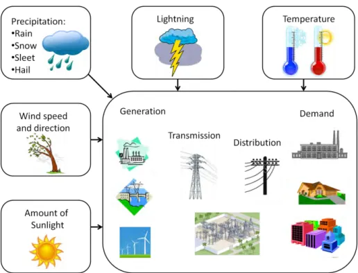
Figure 1: Weather factors affecting power system ... 7

Figure 2: ATPDraw model of the tested line ... 14

Figure 3: GIS data framework ... 15

Figure 4: Dataflow during the fault ... 15

Figure 5: Spatio-temporal correlation of traveling wave fault locator data with lightning, GIS and GPS data ... 16

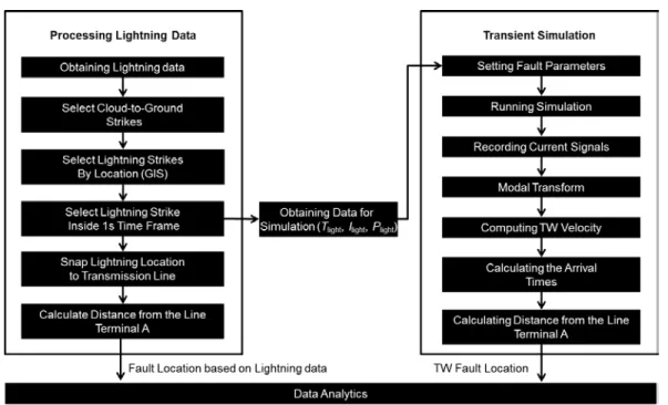
Figure 6: Processing steps ... 17

Figure 7: Buffer around the line ... 17

Figure 8: Selection of lightning strike ... 18

Figure 9: Projecting the lightning ... 18

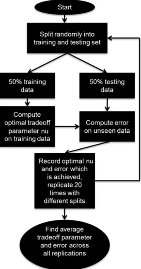
Figure 10: Algorithm flowchart for determining optimal trade-off parameter ... 21

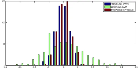
Figure 11: Histogram of an error distribution for individual traveling wave and lightning data; and our approach that combines two methods ... 22

Figure 12: Comparison between traveling wave and lightning data using nu ... 22

Figure 13: Location of three weather stations ... 26

Figure 14: CIGRE concave lightning model, [63] ... 28

Figure 15: The simulation process ... 28

Figure 16: Risk analysis model ... 30

Figure 17: Lightning density map ... 30

Figure 18: Illustration of a network data X = (lightning current, temperature, pressure, humidity, precipitation, BIL_old); Y = (BIL_new); links: impedance matrix. ... 31

Figure 19: Location of transmission network components ... 34

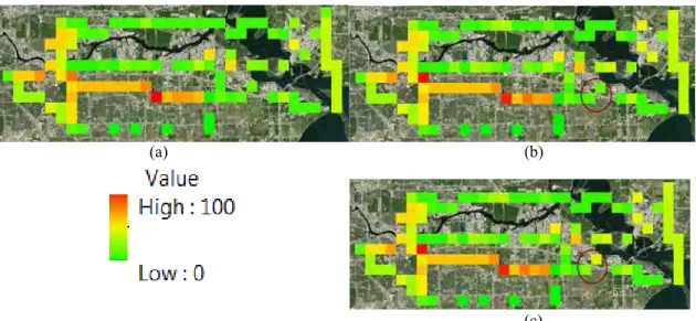
Figure 20: Total risk calculated on (a) January 1st 2009; (b) December 31st 2014; (c) January 5th 2015 (prediction after the next lightning strike) ... 35

Figure 21: Map of the four locations in West Texas ... 40

Figure 22: Wind roses of the four locations in West Texas ... 41

Figure 23: Wind speed density at ROAR 2008-2009 ... 43

Figure 24: Functional boxplot [106] of daily wind speed at ROAR 2008-2009 ... 44

Figure 25: The pressure gradient, Coriolis, and friction forces influence the movement of air parcels. Geostrophic wind (left) and real wind (right) ... 45

Figure 26: Two-layer dispatch model ... 48

(12)

Figure 28: Distribution of forecast errors under different forecast models ... 54

Figure 29: Total operating cost using different forecast models ... 55

Figure 30: Operating cost reduction using different forecast models ... 56

Figure 31: Illustration of the future grid. ... 58

Figure 32: Insert latencies in commercial DBMSs ... 64

Figure 33: Average download speed from various cities to Milwakee ... 65

Figure 34: Structure of denial of services attack ... 66

Figure 35: Example of concurrency management ... 67

Figure 36: CAP theorem by Stephen Smith ... 68

Figure 37: Split file in a distributed file system ... 69

Figure 38: Hash list for distributed databases ... 70

Figure 39: Database sharding... 70

Figure 40: Structure of database simulation ... 72

Figure 41: Simulation of user based clients in the Smart Grid ... 73

Figure 42: Snapshot of reports generated by Prosumer Appliances ... 74

Figure 43: Snapshot of aggregated data grouped by prosumers ... 74

Figure 44: Overall analytics infrastructure ... 75

Figure 45: Performance of HBase on a distributed system... 79

Figure 46: HBase: with and without auto-flushing ... 92

(13)

List of Tables

Table 1: The big data 3 Vs ... 2

Table 2: List of data for improved fault location ... 12

Table 3: The big data properties ... 13

Table 4: List of data ... 25

Table 5:Example of weather data ... 35

Table 6: Site information ... 39

Table 7: MAE values of the 10-minute-ahead, 20-minute-ahead and up to 1-hour-ahead forecasts on 11 days’ in 2010 from the PSS, AR, TDD and TDDGW models at the four locations (smallest in bold) ... 47

Table 8: Generator parameters ... 53

Table 9: Sample days in simulation study ... 53

Table 10: HBase write time with auto flush turned off ... 92

(14)

1.

Introduction

1.1 Project Objectives

The utility industry is encountering new challenges in dealing with extremely large data sets, often called big data. In [1], the authors have denoted that two groups of data can be distinguished: the first group stems from the utility measurement infrastructure, and the second group coming from other source of data not necessarily being part of utility infrastructure.

Examples of the first group of data experienced by the utility industry include the following: (1) synchrophasor measurement system (SMS) data that is used in addition to traditional supervisory control and data acquisition (SCADA) data for situational awareness, (2) data sets collected by poling automated revenue metering (ARM) systems for billing purposes, (3) transient recorder data used for fault location, (4) asset management data that may consist of condition-based measurements collected from intelligent electronic devices (IED) as well as nameplate and maintenance data entered off-line.

The second group of data sets, not obtained through the utility field measurement infrastructure but widely used in decision making, include weather data, Geographic Information System (GIS) data [2]-[4], data from the National Lightning Detection Network (NLDN) [5], landscape and vegetation data [ref], and electricity market data [6]. From [7], correlation of data in time and space and providing unified and generalized modeling, is essential in implementing data analytics for various electric utility applications.

The objective of this research is to illustrate the correlation of various data sets in order to satisfy specific requirements for data analytics in the electric power industry.

1.1.1 The Challenge of the Big Data Integration

The big data exhibits following characteristics, [7], [8]:

• Large volume: describes the quantity of collected data that can reach several gigabytes or even terabytes,

• High velocity: describes the rate at which data is collected and processed typically expressed in terms of number of samples per second,

• Increasing variety: describes the heterogeneity of analyzed data including many different data sources that follow different standards for data representation. Table 1 lists estimation for big data characteristics of several data sources that are of interest for electric utilities. One may see that the amount of data and velocity with which the data is generated can be overwhelming for both on-request and real-time applications.

(15)

1.2 Targets of Research

1.2.1 Outage and Asset Management

The integration of weather data, condition based maintenance data and real-time substation IED data correlated within a geographic context can lead to improved outage and asset management decision-making. Useful data for the integration are:

• Geographic information about utility network asset placement; • Condition based maintenance data for assets;

• Substation IED data concurrent to the lightning strikes that affected the network. Additional data that is used to correlate the events are:

• Geographic Information System (GIS) data; • Data from weather stations;

• Data from the National Lightning Detection Network (NLDN).

The goal of this effort is an integration of relevant data within a single unified model and an investigation of using such modeling to improve outage and asset management decision-making. Following are the outcomes of the research:

Table 1: The big data 3 Vs

VOLUME VELOCITY V A R I E T Y

Smart meters 0.5 million devices can generate more than 120 GB of data per day

Collecting meter data at the interval of 5-15 min

Synchronized phasor measurement

100 devices can collect more than 2.5 GB of phasor data per day

Up to 240 samples per second

GIS and GPS

data Additional GIS layer for every type of data GPS time tag accuracy of 100ns Weather data Only one radar can generate over 50 GB of

data per day New data every 1 to 10 min Seismic data Up to 200 GB of raw _{imagery per day} Sample rate from 0.01 to 100 _{samples per second}

(16)

• Ability to evaluate performance of traveling wave fault location technique in the presence of lightning strikes and severe storms. This investigation is conducted to explore how additional data gathered from unconventional sources can improve the performance of this technique. Additional data can improve accuracy of the traveling wave fault location.

• Methodology for predicting impact on transmission line insulators, power and instrument transformer bushings, surge arresters, etc. Probability of failure after repeated lightning strikes is calculated predicting damage caused by the fault and overvoltage transient flashovers. Maintenance scheduling optimization approach based on risk based calculation. The risk based approach allows the crew scheduling prioritization for minimum cost and maximum improvement of asset reliability

1.2.2 Short-term Spatio-Temporal Wind Forecast

This segment of the project seeks a novel statistical wind power forecast framework, which leverages the spatio-temporal correlation in wind speed and direction data among geographically dispersed wind farms. Critical assessment of the performance of spatio-temporal wind power forecast was performed using realistic wind farm data from West Texas. It was used to justify whether spatio-temporal wind forecast models are numerically efficient approaches to improving forecast quality. The integrated forecast and economic dispatch framework was tested in a modified IEEE RTS 24-bus system. This research included the following detailed targets:

• Develop power system scenarios (day-ahead market operation scenario, intra-day operation scenario, and real-time market operation scenario) for the scheduling models. The advantages and disadvantages for various wind generation forecast models (PSS model, AR model, TDD model and TDDGW model) need to be evaluated.

• The wind data as well as the geographical and pattern information from West Texas needs to be processed to prepare for large scale simulation and model training. • Based on the established benchmark system and power system scheduling, we have

to conduct comprehensive numerical experiments for auto-correlation and cross-correlation analysis.

• We have to design a scheduling system to simulate the established benchmark system. With the scheduling system, we can compare the performance of different models in power system operation by incorporating spatio-temporal wind data. The benchmark system is a revised IEEE RTS system. We reconfigure the system parameters to mimic the electric power system in West Texas region. The system structure, resources mixture, load profiles as well as operating procedure of Texas are required to be well prepared for the scheduling system.

(17)

1.2.3 Distributed Database for Future Grid

There are a lot of potential applications for the data obtained from smart meters. Past experience particularly from blackouts has shown that there is a need for an enhanced decision making process, especially for the following:

• Tracking faults and defects in the system

• Utilizing intermittent power from renewable resources • Outage management and restoration

• Monitoring voltage stability or oscillations

Data obtained from the various smart meter installations makes this a viable problem to solve. The first step involved however is to build a robust data management system that is able to process and store this data and make it available for analysis (either real-time or batch) in an easy to access format. We studied the feasibility of utilizing open source distributed database systems like HBase and Cassandra for storing the data.

1.3 Report Organization

The report is organized as follows: Section 2 provides background for data integration. In Section 3 the improved fault location using lightning data for transmission network is presented. In Section 4, a methodology for evaluating risk of insulation breakdown is presented. Section 5 describes big data application to wind power forecast and look-ahead power system dispatch. Section 6 describes implementation of distributed database for future grid. Contributions of the report are listed in the Section 7.

(18)

2.

Technical Background

2.1 Data Sources

2.1.1 Utility Measurements

The SCADA system provides a set of measurements at the substation, including analog measurements such as bus voltages, flows (amps, MW, MVAR), frequency, transformer tap position, status (breaker switching state) signals, etc. The SCADA Data is sent to the energy management system (EMS) every two to ten seconds. New types of data coming from Phasor Measurement Unit (PMU) and IEDs, such as Digital protective relay (DPR), Digital fault recorder (DFR), Sequence of event recorder (SER), and other IEDs, have a much higher sampling rate and are able to record a larger amount of data. In addition, there are different configuration data that are stored together with these measurements.

As described in [9] the unified generalized representation of data and model may be performed in accordance with the standard formats for data exchange. The data exchange standard provides a description of the data syntax. Some examples are demonstrated below: • SCL (IEC 61850-6) provides description for substation equipment and their

configuration as well as data format for IEDs, [10],

• IEEE COMTRADE (IEEE C37.111) describes the data format for exchange of transient data captured by IEDs, [11],

• IEC CIM (IEC 61970) describes format for power system model and SCADA data, [12] and [13],

• IEEE COMFEDE (IEEE C37.239) describes format for event data exchange, [14], • Measurement requirements and common data format for PMUs is described in

IEEE PC37.118.1 [15], while format for communication of phasor measurements is described in IEEE PC37.118.2, [16].

2.1.2 GIS and GPS

Data involved in the power systems decision-making process have two main components, the temporal and spatial. GIS together with GPS enables spatial-temporal correlation as a base for all other data that may be associated or analyzed. As it is stated in [7] the spatial and temporal correlation of data plays an essential role in the process of integrating big data in the electric power industry applications. Spatial correlation of data is done by integrating different data sets as layers of GIS, while GPS is used for time synchronization between events.

Using GIS it is possible to systematically incorporate spatial data from different sources together [17]. Different data sources can be represented as individual layers, making data visualization and management easier. Several important aspects of GIS operation need to be taken into consideration [18]:

(19)

• Landbase Map: This is the data defining the physical features and spatial attributes of system components, and therefore it forms the framework of the overall GIS implementation.

• Data Conversion: For data to be useful it needs to be pre-processed since geographical attributes which are identified through imagery or other sources then need to go through the vectorization process.

• Layers: These are a GIS specific data structures allowing for heterogeneous data sources to be kept distinctly separate and stored in a single file.

Two distinct categories of GIS data, spatial and attribute data can be identified [19]. Data which describes the absolute and relative context of geographic features is spatial data. For transmission towers, as an example, the exact spatial coordinates are usually kept by the operator. In order to provide additional characteristics of spatial features, the attribute data is included. Attribute data includes characteristics that can be either quantitative or qualitative. For example a table with the physical characteristics of a transmission tower can be described with the attribute data.

Any kind of data with a spatial component can be integrated into GIS as another layer of information. As new information is gathered by the system these layers can be automatically updated. Some examples are:

• History of outages for specified components of transmission system, • Lightning detection network data,

• Signals received from IEDs.

GPS is a system of 24 satellites installed by the US Department of Defense. It provides location and time information for GPS receivers located on the Earth. In order to use this service devices such as traveling wave recorders and lightning sensors are equipped with GPS receivers that supply information about longitude, latitude, and altitude, as well as a precise time tag. The latest equipment has a GPS time accuracy of 100 ns with a resolution of 10 ns [20].

2.1.3 Weather Data

With the developed modern science and technology, the measurements and the data collections infrastructure have been particularly designed and gradually improved for increasingly better operational weather forecasts. Not only localized observations (e.g. radar detection of tornados) but also large-scale weather patterns are necessary for predicting the weather over a specific small area.

The main weather factors affecting the power system are presented in Figure 1. Weather conditions have high impact on all parts of electric power system. Main causes of outages are:

(20)

• Combination of rain, high winds and trees movement: in order to completely understand this event several data sources need to be integrated including precipitation data, wind speed and direction, and vegetation data.

• Lightning activity: the faults are usually caused by cloud-to-ground lighting hitting the poles.

• Severe conditions such as hurricanes, tornados, ice storms: in case of severe conditions multiple weather factors are recorded and used for analysis.

• In case of extremely high and extremely low temperatures the demand increases which can lead to the network overload.

In the case of a large blackout, there is typically a combination of factors leading to the outage. For example, 2003 Northeast Blackout started with tree touching the line but then equipment failure led to the cascading distress on the electric grid. After the blackout, lack of good time synchronization system led to a lot of difficulties with investigation. Thus, in order to prevent large blackouts in the future, it is of great importance to connect all factors affecting the grid and correlate them in time and space. Weather impact together with equipment failure causes more than 50% of outages in electric network.

In order to efficiently exploit renewable energy resources such as wind and solar, weather information can be used as a direct indication of potentials for exploitation of these resources present in a targeted area. Energy suppliers are interested in coordinating the traditional power plants and weather-dependent energy sources. Thus, they need accurate predictions of weather conditions in locations where renewable energy plants are located.

(21)

For example, wind speed is crucial for energy production based on wind, while the sun’s angle and cloud coverage are important information for solar based production.

Following factors are measured in a weather station: • Air and soil temperature (min, max, average) • Precipitation

• Wind speed and direction • Lightning characteristics

• Air relative humidity (min, max, average) • Solar radiation

• Pan evaporation • Snow-water equivalent

Metrological stations (i.e. observation sites) worldwide routinely measure the basic meteorological parameters. The discussions below will demonstrate the data property primarily using ASOS, which the major source of automated surface observational data in the U.S. Most ASOS sites are located in the airports and currently there are more than 900 of them in the U.S [21]. The properties of data collection and interpolation are specifically discussed below:

• Data collection infrastructure:

o Sensors: The group of sensors of ASOS is listed in [21] (e.g. Precipitation

Identification Sensor). The specifications for sensor measuring range, accuracy, and resolution in ASOS are discussed in [21]. The requirements regarding sensor exposure and placement are listed in [22]. More information on station instrumentations may be found in [23].

o Data exchange: The standard formats for weather data exchange among

automated weather information systems are described in [24], and the configurations of ASOS network data flow are described in [21].

• Interpolation: Typically weather stations are sparsely located over the area. In order to generate maps with description of weather conditions for the whole area different interpolation techniques need to be applied [25].

Satellites detect different meteorological phenomena and the atmosphere in different temporal and spatial scales. The satellite meteorological detection is passive remote sensing in general, whereas the radar meteorological detection is active remote sensing. Satellites can measure shortwave (solar) radiation and longwave (terrestrial) radiation reflected and emitted by the earth-atmosphere system, respectively. Meteorological variables such as temperature and humidity profiles, cloud fraction, cloud top temperature can be derived from satellite observations. This process is called “retrieval” in remote sensing.

As a ground-based instrument, radar can detect the weather as far as hundreds of kilometers away. Radar detection has been widely applied for short-time weather forecasts. Radars

(22)

can emit radio or microwave radiation and receive the back-scattering signals from a convective system. The strength of radar echo is dependent on the type of hydrometeors and suggestive of the intensity of the convective system, within which precipitation and radial velocity can be retrieved from radar observations.

2.1.4 Lightning Data

The faults are usually caused by cloud-to-ground lighting hitting the poles. Depending on the area, the lightning may be very important in influencing electric power network faults. For instance, the research in UK [26] shows that lightning strikes are the second most common factor in weather-related distribution system faults. Due to predicted changes in operating conditions caused by weather and the change of power system infrastructure the percentage of faults induced by lightning is estimated to increase by 40% by 2080s [27]. In this case to minimize the effects of lightning proper protection of network structure (i.e. ground wires) and equipment (i.e. surge protectors) must be implemented by utilities [28]. The lightning detection network data can be used to correlate information about lightning characteristics with other event data gathered from the substation measurements. This provides better situational awareness during the critical events affecting the system and has the potential to improve automated fault location techniques.

Lightning data is gathered by the sensors that are typically located sparsely over the area of interest. There are three common types of lightning sensors:

• Ground-based systems that use multiple antennas to determine distance to the lightning by performing triangulation.

• Mobile systems that use direction and a sensing antenna to calculate distance to the lightning by analyzing surge signal frequency and attenuation.

• Space-based systems installed on artificial satellites that use direct observation to locate the faults.

Typical detection efficiency for a ground-based system is 70-90%, with an accuracy of location within 0.7-1 km, while space-based systems have resolution of 5 to 10 km, [29]. For example, The National Lightning Detection Network (NLDN) [30] uses ground-based system to detect lightning strikes across the United States. After detection data received from sensors in raw form is transmitted via satellite-based communication to the Network Control Center operated by Vaisala Inc. [31].

When it comes to the way data is received by the utility we can distinguish two cases: (i) the lightning sensors are property of the utility, and (ii) lightning data is received from external source. In the first case raw data are received from the sensors, while in second case external sources provide information in the format that is specific to the organization involved. No matter which source is used the lightning data typically includes the following information: a GPS time stamp, latitude and longitude of the strike, peak current, lightning strike polarity, and type of lightning strike (cloud-to-cloud or cloud-to-ground).

(23)

2.2 The Big Data

The big data processing methodology consists of following steps [32]: • Search

o Implementing advance search process for fast access to data of interest. o Example: Gather all the data related to specific event.

• Machine Learning

o Identifying important information using machine learning techniques such as

classification and clustering.

o Learning from the historical data.

o Example: Learning from historical data about equipment and measurements at

a given location. • Knowledge Extraction

o Extracting knowledge from information using different data mining

techniques.

o Extracting knowledge from the individual data sources without combining

them. Each data set has its individual conclusions.

o Example: Extracting knowledge separately from the lightning detection

network, and separately from traveling wave recorders. • Correlation

o Combine individual knowledge gathered from different data sources to form a

final conclusions and results based on reasoning.

o Example: Correlating data from traveling wave recorders with data about

lightning. • Prediction

o Identifying rules and trends in analyzed data that can be used to predict future

behavior:

o Linear Prediction o Neural Networks

o Example: Predict what may be the response of equipment in the case of

lightning strike in its vicinity. • Visualization

o Provide systematic way of presenting bots data and results. o Geographical and temporal representation.

(24)

3.

Use of Big Data for Improved Fault Location

3.1 Introduction

Traveling wave fault location has been explored in literature [33-40] and claimed to be extremely accurate, which requires data sampling in the kilohertz and even megahertz range. Many utilities have either deployed such fault locators or are in the process of evaluating them. The GPS synchronization between two traveling wave recorders on two sides of the transmission line was discussed in [38-40]. In [41], the real time monitoring of transmission line transients under lightning strikes was presented. Real time electromagnetic transients were measured and correlated with lightning data recorded at the outage location to evaluate the impact on insulation coordination. Such measurements are very intensive exhibiting sampling rates of several megahertz.

Factors affecting accuracy of the traveling wave fault location methods are:

• Estimation of line length is a major cause of error. As it is presented in [33] not knowing exact line length and line topology can lead to the error close to 500 foot (150 m).

• The traveling waveform is assumed to travel at the speed of light, [42]. When it comes to the overhead transmission lines, velocity of the propagated wave is close to that of the light but not quite the same.

• Time stamping must be very precise to make the system work. As it is stated earlier the latest traveling wave fault locators have GPS time tag accuracy of 100ns, [42]. • Wave-detection error due to interpretation of the transient is a major source of error. This error results from misinterpretation of multiple transients and/or reflected transients. This is a significant concern in the case of lightning strikes. Lightning storms with multiple rapid strikes can cause confusion in terms of which transient was associated with which fault, [43]. In [39], the issue of multiple lightning strikes was investigated and it was reported that travelling wave recorders can produce incorrect results in such cases.

• Current transformers (CT) and capacitive voltage transformers (CVT) can affect the accuracy as well. In [44, 45] modeling techniques for transient response of CTs and CVTs are discussed. It has been pointed out that the differences in the length of the cabling from protection CT to the relay room at each end of the transmission line can affect accuracy [42]. Traveling wave fault location method used in this project extracts the traveling wave from the current signals collected on the secondary of CTs. The CTs have enough bandwidth to pass the transients, however they do affect accuracy of the method.

• Accuracy of the method is greatly affected in case of the faults with small inception angles (<5°). For the cases of fault inception at zero crossing, theoretically, no traveling wave from the fault location is generated [46].

This research demonstrates how the use of traveling wave and lightning surge measurements, correlated with data from Geographic Information System (GIS) and Global Positioning System (GPS) may bring major improvements in the outage

(25)

management. The utilities use such additional data types today, but data is processed manually and poorly correlated leading to delayed decisions and inaccuracies. The automated method has to address the big data problem due to heterogeneity of the data sets, as well as the high volume and velocity of data.

Because information coming from the lightning detection network is not a part of the conventional traveling wave fault location system it is not affected by all of the described errors. Thus, lightning detection network data may complement the fault location method and improves the accuracy of a complete system.

3.2 Data

Complete list of data is presented in Table 2, while Table 3 lists the big data properties of the presented application. The problem falls in the group of big data problems for the following reasons:

• Variety: The database includes sampled waveform data combined with reports from traveling wave fault locator units, lightning detection network, and geographical data. The data files come in different formats that are not compatible and information needs to be extracted so that they match the application. For example, lightning detection network provides the location of lightning strikes in terms of coordinates (longitude and latitude), while traveling wave recorder provides the information in terms of distance to the fault from line terminals.

• Volume: The implementation requires analysis of the extensive set of historical data in order to determine tradeoff between accuracy of traveling wave method and enhancement using the lightning data to determine the confidence of the data gathered during the event analyzed in real time. The lightning data is required for the period of time that covers all events from historical data and each lightning report will generate new map. This is just one level at which the volume of data can be overwhelming. In addition, during the fault, extensive set of data is received and

(26)

not all of it is used for automated fault location. First, the important information needs to be extracted in an automated way. Typically, this process is done manually by utilities today. With methods used in big data analysis such as indexing for faster search and machine learning for extracting knowledge from data this process can be automated.

• Velocity: The velocity refers to the speed at which data is arriving to the central computing facility. During the fault, multiple sources will send a large amount of data that needs to be stored and ready for analysis. The examples are samples of traveling wave waveforms and coordinates of lightning strikes.

3.3 Methodology

3.3.1 Traveling Wave Fault Location

The GPS synchronized traveling wave method is used as one source of information for fault location. Traveling wave fault locator calculates distance to fault automatically based on recorded samples of traveling waves at one or both sides of the line. Mostly used method in modern devices is double ended Type D method with GPS synchronization. The locator calculates arrival time of the fault-induced waves using GPS as a reference. Then, these time tags are sent to the central station where fault location algorithm is used to determine distance to the fault from line terminals. In addition, samples of the recorded signal are transmitted. The accuracy of traveling wave method is highly dependent on the sampling rate. Modern devices use sampling frequency of 0.1 to 20 MHz. In case of Type D traveling wave method, GPS is primarily used for synchronization between signals received at two ends of the line. Conveniently, this information can be used for time correlation with lightning detection data that also uses GPS.

In order to implement traveling wave fault location the following steps are taken:

• Modeling of the power system: It is done according to the method given in ref, [47]. Transmission line modeling is done using J. Marti model, [48]. This is a frequency

Table 3: The big data properties

VOLUME VELOCITY V A R I E T Y

Traveling wave data 4 GB for storage of 2100 records from 8

line modules per substation device Baud rate of 115200 bits per second

Lightning data 40 MB of data per day Sensor baud rate 4800 bits per second, _{event timing precision of 1μs}

(27)

dependent line model that uses analog filtering technique for identification of line parameters and can be simulated with ATP EMTP software, [49].

• Simulating the fault transients: Faults are introduced in various locations over the selected transmission line.

• Determining modal transformation for a three-phase system: Signals are transformed into modal components using Clark’s transformation, [50]. After modal transformation a three-phase system is represented by an earth and two aerial modes. The aerial mode 1 is used for fault distance estimation.

• Computing the traveling wave velocity: Method that uses maximum of the first two consecutive peaks of the power delay profile (MPD method, [36]) is used.

• Calculating the arrival time: Wavelet transformation is used to determine the arrival time of the transient peak. The “mother” wavelet that is used is Daubechies wavelet, [37]. Wavelet Toolbox in MATLAB is used [51].

• Calculating fault location: The arrival times of the transient peaks at two TWRs that are located on two line terminals (TA, TB), line length between two TWRs (l)

and calculated velocity of wave propagation (ν) are used to calculate the distance θ

to fault as

(3.1) • Performing time synchronization: Arrival times of two wave fronts are

synchronized using GPS, [38-40].

The model of a 400 kV transmission line presented in Figure 2 is used for simulation in the experimental section. The sampling frequency was 1 MHz. The line length was 120 miles (~193 km). The faults were generated in the range from 10 to 110 miles from the terminal A.

2 ) ( ν θ=l+ TA−TB

(28)

3.3.2 Spatio-Temporal Correlation

Framework for GIS project is presented in Figure 3, [52]. Data collected by lightning detection network and traveling wave recorders is mapped and stored in Geodatabase. Geospatial Analysis Tools are used for manipulation of maps. Framework contains one layer for each type of data. Layers are classes or categories of data that can be organized in separate and distinct data structures, but integrated into a single file. These layers can be updated as the new information arrives to the system.

By comparing time stamps of events detected by traveling wave recorders and those obtained from querying the lightning detection system it may then be determined whether the disturbance is likely to be caused by lightning activity, as indicated by their closeness in time and space. The flow of information is illustrated in Figure 4. If it is determined that the disturbance is likely generated by lightning then the complete set of data about the event is gathered at the Central Station where correlation of data is leveraged together with analytics to improve fault location. In the Central Station the transient simulation of event is run and analysis of data is performed as described next.

Figure 3: GIS data framework

(29)

The data management for the correlation process is shown in Figure 5. Traveling wave fault recorders are located at both ends of the transmission line. On the other hand lightning sensors are typically not a part of the utility infrastructure and are located sparsely across a wide area. The traveling wave fault location system provides the estimate termed

Automatic Fault Location Result in Figure 5. This result is implicitly allocated to the transmission line. Lightning sensors provide an estimated Location of a Lightning Strike. This result is presented in terms of longitude and latitude and it is not necessarily located on the transmission line, but rather somewhere in the vicinity of the line.

In Figure 6 processing steps for traveling wave fault location and lightning data integration are described. Before the beginning of spatio-temporal correlation process lightning data set is reduced to set containing only to-ground surges, where all instances of cloud-to-cloud surges are removed from data set. Then, the temporal correlation is done. After fault is detected, the time window that contains 2 seconds around the time stamp for fault beginning received from the traveling wave recorder (FaultStart) is created. The data received from lightning detection network is searched and only lightning strikes that satisfy following rule are collected inside the Database A:

|𝐹𝐹𝐹𝐹𝐹𝐹𝐹𝐹𝐹𝐹𝐹𝐹𝐹𝐹𝐹𝐹𝐹𝐹𝐹𝐹 − 𝐿𝐿𝐿𝐿𝐿𝐿ℎ𝐹𝐹𝑡𝑡𝐿𝐿𝑡𝑡𝐿𝐿𝑡𝑡𝐿𝐿𝑡𝑡𝑡𝑡𝐹𝐹𝐹𝐹𝐹𝐹𝑡𝑡𝑡𝑡| < 1𝑠𝑠 (3.2) After that the spatial correlation is done. Based on location of line terminals and geographical representation of the line the buffer around the line is created that covers area going 300m on both sides of the line, Figure 7. This area has a shape of a polygon. The data in Database A is searched and only those lightning instances that are inside the buffer area are collected in Database B.

Figure 5: Spatio-temporal correlation of traveling wave fault locator data with lightning, GIS and GPS data

(30)

In the next step lightning instances from Database B are searched and the closest one to the traveling wave recorder result is chosen to be correlated as a LightningDetectionResult,

Figure 8. The location of the lightning strike is projected to the closest point on the transmission line using a “snap” feature, Figure 9. The snap editing in GIS will move the point within the specific distance (tolerance) of the line to the closest point on the line. This snapped point is considered as the lightning detection network estimate of fault location so that the fault location can be described in terms of distance from the line terminals. For the tolerance 1 km distance from the line is chosen. Only lightning strikes that are within 1 km from the line will be used in the correlation process. Then, two fault location results one coming from the traveling wave fault locator and the other coming from the lightning

(31)

detection network are combined using a Bayesian framework in order to improve the accuracy of the prediction.

3.3.3 Data Analytics

We consider the traveling wave fault location to be the main source of information about the fault event. It processes the recorded data x, and makes the maximum likelihood estimate of the fault location based on this data. The precise value from (3.1) may be described as the following,

Figure 8: Selection of lightning strike

(32)

(3.3) It is possible to discern the variance of θ either from historical records or through other means, but these methods may be unreliable and are beyond consideration in this study. The lightning detection data is considered the prior probability, in this case coming from indirect, side-information and independent of the measurements x,

(3.4) The posterior probability of the fault location can then be expressed using Bayes Theorem as,

(3.5) In order to compute the necessary maximum a posteriori estimate of fault location,

(3.6) it is not necessary to compute the normalization constant because the same fault recorder data x is considered under all fault location positions θ.

By considering the posterior instead of only the likelihood better predictions are made because cross-domain data is integrated.

Taking the logarithm of the (3.5) and disregarding the normalization constant,

(3.7) Under the normal assumption for both distributions prior and likelihood in (3.6), the explicit computation of variance is not necessary. Instead it is computationally favorable to compute the optimal trade-off parameter nu from the interval [0, 1]. This parameter then controls the trade-off between a bigger or smaller variance in , and , but only in direct proportion to each other and irrespective of p(x). At nu = 1 we completely trust the lightning detection network data, and then as nu is transitioned towards 0 more and more certainty is placed in the traveling wave fault location.

This approach is computationally favorable to fully Bayesian approaches such as Markov Chain Monte Carlo sampling, which would make the application infeasible for power systems.

Considering the monotonicity of the logarithmic function we may express the improved fault location as the linear combination of

( ) ( )

( )

x p p x p x pθ = θ θ ) (x p

( )

θx p

( )

xθ p

( )

θ p ~log log log +

( )

xθ p p

( )

θ

(33)

(3.8) The task becomes that of obtaining the precise nu to use. In order to compute nu a binary search along a line can be used to find optimal values since the problem is one dimensional. This process requires only O(log n) time to find the optimal nu among n given values. A simple linear combination like this has the advantage of high bias and low variance in machine learning terms, meaning that its predictions are not likely to be very imprecise in addition to having good generalization power across unseen examples. Because of the low computational complexity this kind of algorithm is directly applicable to big data scenarios.

3.4 Results

In order to assess the performance of the proposed fault location method it was necessary to evaluate its performance on a number of different fault scenarios. Using the model in Figure 1, 1000 fault scenarios were simulated. First, all fault scenarios were solved using only the traveling wave method for fault location. After simulation the error of this method was calculated as the relative mean absolute error,

(3.9) Second, the results from the lightning detection network were calculated as explained in section 3.3 and (3.9) was used to quantify the error.

Algorithm flowchart for testing the proposed method is presented in Figure 10. First the dataset is split into training and testing set. Training data is used to compute the optimal tradeoff parameter nu. Error is then calculated using testing data.

After correlation of the two methods, as it was explained in Section 3.3.2, error of the improved result was calculated using (3.9). When dealing with a linear combination of predictors it is necessary to assess the generalization performance. Good generalization is indicated by the ability of a fault location method to locate faults accurately even for unforeseen fault locations. In order to quantify the generalization performance of the proposed fault location method it was necessary to compute the generalization error. In order to estimate the generalization error of the improved fault location method it is necessary to split the data from many different scenarios into a training set and a testing set of data. Determining the optimal nu on the training set gives point estimates of the generalization error on the testing set when comparing the improved fault location to the true fault location, and therefore the procedure needs to be repeated for precise estimates, a process often calls for 2-fold cross-validation. The results in Figure 11 and 12 are average results, computed per scenario, from 100 replications of cross-validation.

( ) ( ) [ ] [ ( )] [ θ θ ] θ θ θ θ p nu x p nu x p nu ⋅ + − ⋅ = ) 1 ( max arg max arg max arg log max arg

(34)

A histogram of all three results is presented in Figure 11, where the x-axis represents the error and the y-axis represents the frequency of that error, where errors from different scenarios are binned according to a regular grid. From Figure 11, the proposed approach outperforms the traveling wave fault location, having the largest number of test cases with error that is closer to zero. For every test case our approach shoved better accuracy than the individual methods. Mean Square Error of distance to fault for the lightning data was 0.0076±3.1e-04 miles, for traveling wave it was 0.0012±4.3e-05 miles and the improved method showed 0.0011±4e-05 miles, both the variance and the mean of the error were smaller using the improved method on unseen fault scenarios, when compared to the traveling wave method.

3.5 Discussion

It is significant that the traveling wave method result has much higher accuracy than the one obtained from lightning data. The lightning detection data may only be useful in

(35)

enhancing the traveling wave fault detection method. Lightning data has very high variance as well compared to other two methods.

Additionally, the proposed method shows no bias in the predictions in Figure 10, indicating that the fault prediction location neither systematically over- or under-estimated. Because traveling waves are recorded on both sides of the transmission line, the error does not depend on the distance from the fault.

As it can be seen in Figure 12 the tradeoff parameter nu between accuracy of traveling wave method and lightning data is estimated to be optimal at 0.871±0.0133 on unseen examples. This can be interpreted as placing 87.1% trust in the result of the traveling wave method, 12.9% in the estimate from lightning. The low variance of nu is indicative of the low variance predictor used for improved fault location.

Figure 11: Histogram of an error distribution for individual traveling wave and lightning data; and our approach that combines two methods

-0.40 -0.3 -0.2 -0.1 0 0.1 0.2 0.3 0.4 0.5 50 100 150 TRAVELING WAVE LIGHTNING DATA PROPOSED APPROACH 0 0.1 0.2 0.3 0.4 0.5 0.6 0.7 0.8 0.9 1 2 4 6 8 10 12 14 16x 10 -3

lightning data traveling wave

M ean S quar e E rror nu

(36)

3.6 Summary

The research demonstrates that correlating automatically multiple sources of data may help enhance fault location calculation. A method using correlation of cross-domain data for identifying which faults are likely to be caused by lightning strikes is presented. A method for locating faults using lightning detection data is presented and its precision quantified. A method of integrating lightning detection sensor data with traveling wave fault location measurements is presented and its precision quantified. The results indicate that integrating lightning detection sensor data with traveling wave fault detection data improves fault location accuracy. Proposed method that correlates traveling wave fault locator data and lightning data exhibits better performances than any of the methods alone.

(37)

4.

Evaluating Impact of Weather Events to Insulation Coordination

4.1 Introduction

Lightning studies and experiences with insulation coordination have been reported in [53-57]. For the purpose of estimating probability of a lightning strike, historical lightning data has been used in [53, 54]. In [41], real time monitoring of transmission line transients under lightning strikes was presented, which allows for spatio-temporal correlation of lightning data and transient measurements to evaluate the impact on insulation coordination. Correction factors for utilization of weather station data for insulation coordination have been described in [58]. In [59], the lightning-related risk analysis using artificial neural network in order to estimate insulator flashover rates has been performed. An optimization procedure to determine locations of line arresters that would minimize the risk has been implemented. In the mentioned work, the weather conditions have been taken into account; however, the statistical study has been performed based on a randomly generated data. This paper builds on the study presented in previous chapter by adding the risk assessment to improve transmission system asset and outage management. The approach utilizes the weather data used for improved fault location to determine how the lightning protection assets deteriorate due to high frequency transients caused by lightning. By evaluating how past lightning strikes affect the condition of the equipment over time, quantitative means for prediction of potential insulator failure are derived allowing the measures that can be taken in order to improve lightning protection performances of the system to be specified. The overarching goal of this research is to develop an early warning system (EWS) for prediction of insulation breakdown. The aim is to develop a risk-based EWS that can integrate real time data about lightning threats to the system, and determine system vulnerability of and economic impacts on a given area of interest. In today’s practice the vulnerability of the system’s components is determined in advance by the manufacturer after performing certain number of standardized tests under controlled conditions. The stress limit determined through the tests is assumed to be constant during the component’s lifetime. In our research, accumulated impacts of past disturbances to the components are taken into account to assess unfolding component’s vulnerability after exposure to continued weather threats such as lightning. In order to evaluate the current state of equipment as well as prediction of risk in case of future weather impact, a case with real data gathered from lightning detection network and weather stations is conducted.

4.2 Data

A complete list of data used in this study is presented in Table 4. All towers and substations were geographically referenced in order to spatially correlate their locations with those of lightning strikes and weather stations. The 100 m buffer is created around transmission lines. Only lightning strikes inside the buffer were selected and each of them was simulated as one fault scenario inside ATP. Location of lightning strike in the ATP model is

(38)

Data obtained from three weather stations was used: Station NCHT2 - 8770777 - Manchester, TX, Station LYBT2 - 8770733 - Lynchburg Landing, TX, Station MGPT2 - 8770613 - Morgans Point, TX, [60]. The locations of stations are presented in Figure 13. Each weather station reports measured values at the location with certain time resolution.

4.3 Methodology

4.3.1 Integrating Weather Data

After values from multiple weather stations are collected, interpolation algorithms are used to estimate the values of parameters in an area of interest (i.e. transmission lines). The results are then presented as a vector or raster maps than can be overlaid with the network georeferenced map. Time instances of interest are times of lightning strikes obtained from lightning detection network. In order to temporally correlate lightning data with data from weather stations, linear interpolation is used. For each tower and substation, weather parameters at the locations were calculated based on distance to the weather stations as:

P = P1 d1+ Pd22 + Pd33 1 d1+ 1d2+ 1d3 (4.1)

Table 4: List of data

Lightning Detection Network

Weather Insulation Studies Geography Traveling

Wave Fault Locators

Date and time of

lightning strike Temperature Surge impedances of towers Location of substations Date and time when event was recorded Location of a

strike (latitude and longitude)

Atmospheric

pressure Surge impedances of ground wires Geographical representation of the line

Distance to the fault from the line terminals Peak current and

lightning strike polarity

Relative

humidity Footing resistance Location of towers Transient signals recorded at the line terminals Type of lightning strike (cloud to cloud or cloud to ground)

Precipitation Components BIL (Basic Lightning Impulse Insulation Level)

Location of surge arresters

(39)

where P is an estimated parameter value at the component location, Pi is a parameter value

measured at weather station i; and di is a distance from the weather station i to the

component. Weather data is used to calculate BIL under nonstandard atmospheric conditions [61], BILA as:

(4.2) where BILA is the BIL under nonstandard conditions, BILS is the standard BIL, δ is the

relative air density, and HC is the humidity correction factor. Relative air density can be

calculated using:

(4.3) where TS and PS are standard temperature and pressure respectively; T and P are measured

temperature and pressure respectively. Humidity correction factor is equal to 1 for rainy conditions and for dry conditions can be calculated using:

(4.4)

4.3.2 Network Modeling

The network is modeled using the ATP version of EMTP [49]. J. Marti’s frequency dependent model [48] was used for modeling of transmission line segments between towers. For representing towers, multistory transmission tower model for lightning surge analysis proposed in [62] is used. Tower model parameters are calculated using (4.5.a-4.5.f): S C A H BIL BIL =δ T P PT S S = δ     ₋ ⋅ + =1 0.0096 11 δ H HC

(40)

Zt = 60�lnH_r −1� (4.5.a) r =�r1h1+ r2h2_2H + r3h3� (4.5.b) H =�hi 3 i=1 (4.5.c) Ri =_h−2Z₁_+ht₂ln√γ_+h₃hi, i = 1. .3 (4.5.d) R4 = −2Ztln�γ (4.5.e) Li =αRi2H Vt , i = 1,4 (4.5.f) where: Zt – tower impedance, H – tower height, Ri – resistances of sections, Li – inductances of sections, γ – attenuation coefficient, α – damping coefficient, Vt – propagation velocity,

h1, h2, h3 – distances between stories,

h4 – distance between lowest story and ground,

ri – distances between tower center and tower edge at the level of a story i.

Rf – tower footing resistance.

Modeling of lightning impulse is done using current source based on CIGRE concave lightning model presented in Figure 14 [63]. Lightning peak current is obtained from the lightning detection network. A time characteristic is synchronized with the time of a lightning strike.

(41)

The simulation process is presented in Figure 15. First the lightning strike is selected and data from lightning detection network are sent to the ATP model in order to generate the fault. Then the simulation is run. After simulation for each node (tower) of interest, the maximum value of voltage is recorded. In parallel, the nonstandard BIL for the component is calculated using weather data. In the end, measured maximum voltage is compared to the component’s nonstandard BIL and data is sent to the prediction model where it will be used as historical data for training.

(42)

4.3.3 Risk Framework

Risk assessment framework is defined as follows:

(4.6) where R is the State of Risk for the system (or component), T is the Threat intensity (i.e. lightning peak current), Hazard P[T] is a probability of a lightning strike with intensity T;

P[C|T] is the Vulnerability or probability of an insulation breakdown if lightning strike with intensity T occurred; and the Worth of Loss, u(C), is an estimate of financial losses in case of insulation breakdown.

The proposed risk measure can be defined as a stochastic process and referenced in time and space as follows [64]:

R(X, t) = P[T(X, t)]∙P[C(X, t)|T(X, t)]∙u(C(X, t)) (4.7)

where X represents the spatial parameter (longitude and latitude) and t represents the time parameter obtained using GPS. As an example, the impact of lightning is associated with certain time and location. The impact that lightning will have on a component depends on the component’s distance from the lightning strike. With the stochastic risk maps, the early warning system can be spatially and temporally mapped accordingly.

The spatio-temporal risk measures fit well with Bayesian paradigm [64]. The definition of Bayesian model is:

π(hypotesis|evidence) =

(4.8)

= f(dobs|θ)π(θ)

∫f(dobs|θ)π(θ)dθ∝ βf(dobs|θ)π(θ)

where π(θ) is the prior state of information or probability of the evidence associated with the set of parameters θ; f(dobs|θ) is the likelihood of evidence or parameters θ will reproduce

the observations dobs; π(θ|dobs) is the posterior representing joint probability function

between prior and likelihood.

Figure 16 shows the relationship model for risk assessment. Lightning data are indicating the probability of a lightning strike that is impacting probability of a backflashover. Probability of a backflashover is also under impact of weather conditions (temperature, pressure, humidity and precipitation). If there was a backflashover, the probability of a component failure is increased. Due to component failure, some losses are expected to be imposed. The chain of events will impact the final risk as discussed in [64] when using Bayesian Networks. The three components of risk analysis (hazard, vulnerability and worth of loss) can be identified in Figure 16 and are explained in the following sections.

) ( ] [ ] [T