Application of Artificial Neural Network and Adaptive Neural based Fuzzy Inference System Techniques in Estimating of Virtual Water

Application of Artificial Neural Network and Adaptive

Neural-based Fuzzy Inference System Techniques in

Estimating of Virtual Water

Khaled Ahmadaali

Department of Irrigation & Reclamation Engineering, Faculty of Agricultural Engineering & Technology,

University of Tehran, Karaj, Iran.

AbdolMajid Liaghat

Department of Irrigation & Reclamation Engineering,

Faculty of Agricultural Engineering & Technology, University of Tehran, Karaj,

Iran.

Nader Heydari

Irrigation and Drainage Department, Iranian Agricultural Engineering Research Institute (AERI),

Karaj, Tehran, Iran.

Omid Bozorg Haddad

Department of Irrigation & Reclamation Engineering,

Faculty of Agricultural Engineering & Technology,

University of Tehran, Karaj, Iran.

ABSTRACT

Wheat, barley, sugerbeet, potato, alfalfa, and corn are common crops produced in Iran, which need the most virtual water volume compared to other crops. Determination of the virtual water for these crops would assist in better management of water resources. The main objective of this study is to find out the best technique for estimating and mapping of virtual water. In this research, the virtual water volume was determined by crop water requirement and crop yields using three ANN structures as well as ANFIS technique. Based on RMSE and R2 the comparison of obtained results predicted through the applied ANNs structures indicate that the RBF outperforms the other models for estimating virtual water for wheat, potato, corn, and barley. Moreover, a comparison between RBF and ANFIS revealed that ANFIS is a promising model, which can be efficient mathematical tool for estimation of crop‟s virtual water.

Keywords

virtual water, ANN, MLP, RBF, GRNN, ANFIS

1.

INTRODUCTION

Iran is located at an arid and semi-arid region with low precipitation and high evapotaranspiritation. Moreover the distribution of water resources availability is uneven spatially and temporally, so that the central, eastern and southern part of the country faces drought. Also in the absence of irrigation, rainfed agriculture has a high risk. The average annual precipitation is about 252 mm, but the average annual evaporation capacity is about 1500-2000mm. regarding the evaporation capacity, 71% of annual precipitation about 179mm vaporize directly. The regional actual water use is 87.5×109 m3, of which agricultural irrigation water accounting for 94.25%, and urban water 4.75 and industrial water use 1% (Alizadeh and Keshavarz, 2005). The specific climate condition led to unsuitable temporal and local precipitation hence, producing sustainable agricultural products which subject to the proper use of water resources. Growing population and urbanization have increased required water and food unexpectedly in the country. Considering the mentioned climate conditions and limitation of using new water resources, and on the other hand the necessity of increasing agricultural products, considering Virtual Water (VW) content of these products is vital to manage the water resources.

The concept of virtual water which is a method of studying water resources quantitatively was hypothesized by Tony Allan (1997) for the first time, to describe the total water embedded in agricultural products suggesting that water poor region should import water-intensified agricultural products. Various studies conducted the world show the direct effect of virtual water on water management and its direct and indirect effects on agriculture as the major consumer of water resources. Measuring virtual water is a useful concept for assessing water management as it permits the comparison of crops and livestock from the perspective of embedded water (Brown et al., 2009). A number of studies have recognized the usefulness of virtual water concept to analyze production patterns and associated water flows(Dietzenbacher and Velázquez, 2007; Zeitoun et al., 2010).

Wheat, barley, sugerbeet, potato, alfalfa, and corn are the major crops produced in Iran. Unfortunately, these crops are also those with the highest Virtual water content (VWC) compared to other crop commodities. Determining VW of these crops would help the decision makers to manage water resources better. The „virtual water‟ perspective is consistent with the concept of integrated water management in which many aspects of water supply and demand or consider when determining the optimal use of limited water resources (Bouwer, 2000).

In recent decades, inspiring of swarm intelligence concepts has been increasingly proliferated in the field of water resources by developing different approaches. Ease of use and availability of such methods have been fundamental reasons for their popularity. Moreover, these methods are capable to be used by the minimum level of the available data.

of any unstudied area without any need of costly measurements or time consuming calculations.

With regarding to the literature review and to the best of our knowledge, VW has not been used in earlier papers. In this study, efficiency of three different ANN techniques, Multilayer Perceptron (MLP), Radial Basis Functions (RBF), and Generalized Regression Neural Networks (GRNN) as well as ANFIS were examined in estimation of VW using measured data of the yield and Crop Water Requirement (CWR) of common crops, and climatic factor data in Iran.

2.

DESCRIPTION OF THE STUDY

AREA

Iran is one of the biggestcountries of the Middle East in terms of area at 1,648,195 km2 (636,372 sq mi), and is located between the 25°N - 40°N latitudes and 44°E - 64°E longitudes with altitude from -40 m to 5670m. Winter temperature of -20 C and less in most part of the high altitude regions and summer temperature of 50 C in the southern regions of Iran have been recorded (Montazar and Zadbagher, 2010). Distribution of precipitation incountry is not uniform and causes problems for supplying water invarious regions especially in populated areas.

3.

MATERIAL AND METHODS

3.1 Virtual water calculation

The data of irrigated cropped area (ha) and crop yield data (t/ha) for mentioned major crops are taken from ministry of agriculture. The actual crop evaporation per crop have been done based on FAO Penman-Montieth in non-standard condition and so effective rainfall (Peff) data is collected from

water national document. The plain‟s Geographic Information System (GIS) data file is taken from the ministry of energy. Latitude, longitude, and altitude of these plains are derived from Digital Elevation Model (DEM) (100×100m) from National Cartographic Center of Iran. The database contains 364 points throughout the country‟s latitude, longitude, altitude, and VWC of the major crops prepared and was analyzed by mentioned models. CWR have been calculated with the methodology developed by FAO as formula 18 (Allen et al., 1998a; Allen et al., 1998b) states

(1) ETc = Kc× ET0

where𝐸𝑇𝑐 mm is the actual crop evaporation, Kc is the crop

coefficients, and ET0 mm is the potential crop evaporation.

CWR m3/ha can be calculated in accordance to formula 2:

(2) CWR = 10(ETc− Peff)

wherePeff is the effective rainfall. The factor 10 is to convert

mm into m3/ha.

VWC of each crop can be computed as (Fang et al., 2010):

(3) VWC𝑐 =CWR_Y 𝑐

𝑐

where𝑉𝑊𝐶𝑐 stands for the VWC of unit crop c (m3/t), 𝐶𝑊𝑅𝑐

is the water requirement of unit crop c (m3/ha), and 𝑌𝑐 refers

to the annual average yield of unit crop c (t/ha). A summary of obtained results and their basic statistics was presented in Table 1.

Table1. Statistical analysis of the used parameters

Latitude

(m)

Longitude (m)

Altitude (m)

Virtual water (m3/t)

Wheat Barley Alfalfa Potato Corn Sugerbeet

Maximum 1,683,671.80 4,396,919.30 2,756.00 2,967.00 2,984.10 3,522.10 2,224.30 706.6 1,263.00

Minimum -72,251.40 2,871,535.90 -8 559.5 548.3 930.5 107.5 117.3 107.3

Range 1,755,923.10 1,525,383.40 2,764.00 2,407.50 2,435.80 2,591.60 2,116.70 589.3 1,155.70

Skewness 0.2 0 -0.2 1.3 0.9 1 1.8 0.9 1.7

Kurtosis -1 -1.1 -0.3 1.5 0.9 1.4 3.7 0.6 3.7

Mean 699,196.00 3,609,192.70 1,257.10 1,322.50 1,346.20 1,713.60 601.7 284.4 418.6

Std. dev. 452,006.00 375,024.70 577.9 479.9 459.4 467.2 391.8 115.3 200.8

3.2 Artificial neural networks (ANNs)

ANNs are based on current understanding of biological nervous systems, though much of the biological details are neglected. ANNs are massively parallel systems composed of many processing elements connected by links of variable weights (Aali et al.,2009). There are well known networks with specific architecture which are wieldy used in water resources engineering. Three different program codes were written in MATLAB 7.11.0 R2010b for ANN models simulations.

3.2.1 Multi-layer perceptron neural

network (MLP)

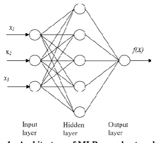
Fig 1: Architecture of MLP neural network

Basically the MLP consists of three layers: the input layer, where the data are introduced to the network; the hidden layer, where the data are processed (that can be one or more), and the output layer, where the results for given inputs are produced. The weights are computed through an iterative process based on back propagation algorithm in such a way that the difference between computed and given output (or any error criterion such as mean square error) is sufficiently small. The hidden layer node numbers of each model were determined after trying various network structures, since there was no theory yet available to tell how many hidden units were needed to approximate a given function. Cross validation mode (checking mode) monitors the error to find the optimal termination point for training and also avoid overtraining. Testing mode was used to determine how accurately the network can simulate input-output relationships (Aali et al., 2009).

All collected data were divided into three sets; training, validation, and test data. Each set has the various percents of all data and finally the best set with the best percentage were determined. In this study a having a three-layer feed-forward network that consisted of an input layer, one hidden layer, and one output layer. Tangent sigmoid and linear transfer functions were used for hidden and output layers respectively.

3.2.2 Radial basis function neural

network (RBFNN)

Radial basis function is the basis for RBFNNs, which are in turn the basis for series of networks known as statistical neural networks. An RBFNN, which is a three layer network with one hidden layer, uses the similarity between observations of predictors and similar sets of historical observations to obtain the best estimate for a dependent variable (Figure 2).

Fig 2: Architecture of RBFNN

The number of neurons in hidden layer was equal to the number of historical observation of predictors which each neuron in this layer represent the pair of historical observation of predictors/dependants. The output of each neuron was actually the contribution of the historical observation in estimating the real time event The kernel function which is Gaussian kernel function is used to calculate the outputs; the input is the Euclidian distance between each input to the neuron, the specified vector of the same size of the input (Wang et al., 2010). For each input x, the j-th output (j=1, 2, ...,L), 𝑦𝑗(𝑥) , defined as:

(4) yj(𝑥) = 𝑂𝑗𝑖exp⁡(− x − Ci

2

2σ𝑖2 𝑀

𝑖=1 )

where Oji = the synaptic weight between the i-th neuron of the

hidden layer and the j−th neuron of the output layer, M, L, respectively denotes the number of the hidden neurons and the number of the output neurons, || ... || represents Euclidean norm, and 𝜎 = the controlling parameter of the kernel function which output limits are dependant.

3.2.3 Generalized regression neural

network (GRNN)

A GRNN is a variant of the radial basis function network. A GRNN consists of four neuron layers: input, pattern (radial basis), summation, and output layers that are shown schematically in Figure3 (Shahlaei et al., 2010).

Fig 3: Architecture of GRNN

In this network, number of neurons in the input and output layers were equal to the dimension of input and output vectors respectively. GRNN is a universal approximator for smooth functions, which is able to approximate any relationship between X-block and its y vector. The operation of approximation of y vector by network was performed during training of network. After figuring out the relationship between input and output of networks, this relationship was used for computation of output of networks. In the GRNN model, approximation of an output vector with respect to an X-block can be regarded as finding the expected value of y conditional upon the X-block.

3.3 Adaptive Neural-based Fuzzy Inference

System (ANFIS)

2009). The first-order Sugeno fuzzy model, a typical rule set with two fuzzy If-Then rules, can be expressed as:

(5) Rule 1: If x is A1 and y is B1, then

𝑓1= 𝑝1𝑥 + 𝑞1𝑦 + 𝑟1

(6) Rule 1: If x is A2 and y is B2, then

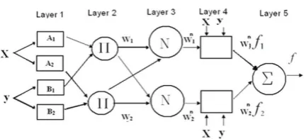
𝑓2= 𝑝2𝑥 + 𝑞2𝑦 + 𝑟2

The corresponding equivalent ANFIS architecture is presented in Figure 4.

Fig 4: Equivalent ANFIS architecture

Nodes at the same layer have similar functions. The node function is described next. The output of the ith node in layer l is denoted as Oli.

Layer 1: Every node i in this layer is an adaptive node with node function

(7) Ol,i= μAi x i = 1,2

Ol,i= μBi−2 y i = 3,4

where x (or y) is the input to the ith node, and Ai(or B i-2) is a

linguistic label (such as „„low‟‟ or „„high‟‟) associated with this node. In other words, Oli is the membership grade of a

fuzzy set A (= A1, A2, B1,or B2) and it specifies the degree to

which the given input x (or y) satisfies the quantifier A . The outputs of this layer are the membership values of the premise part.

Layer 2: This layer consists of nodes labeled П, which multiply incoming signals and sending the product out. For instance,

(8) 𝑤𝑖= 𝜇𝐴𝑖 𝑥 × 𝜇𝐵𝑖 𝑦 𝑖

= 1,2

Where, each node output represents the firing strength of a rule.

Layer 3: In this layer, the nodes labeled N calculates the ratio of the ith rule‟s firing strength to the sum of all rules‟ firing strengths

(9) 𝑤𝑖=_𝑤 𝑤𝑖

1+ 𝑤2 𝑖 = 1,2

the outputs of this layer are called normalized firing strengths. Layer 4: This layer‟s nodes are adaptive with node functions

(10) 𝑂𝑖4= 𝑤𝑖𝑓𝑖= 𝑤𝑖(𝑝𝑖𝑥 + 𝑞𝑖𝑦 + 𝑟𝑖)

whereWi is the output of layer 3, and{pi, qi, ri}is the

parameter set. Parameters of this layer are referred to as consequent parameters.

Layer 5: This layer‟s single fixed node labeled

Σ

(11) 𝑂15= 𝑤𝑖𝑓𝑖

𝑖

= 𝑤 _𝑤𝑖 𝑖𝑓𝑖

𝑖 𝑖

In the present study, the triangular (trimf), trapezoidal (trapmf), gaussian (gaussmf), generalized bell shaped (gbellmf), and sigmoid (sigmf) membership functions (Laslett et al.) were used for input data. For output data the constant and linear membership function were used. A10-fold cross validation method was used for selecting the best performing models during the training process. Two optimization method Back propagation and hybrid were used. In each application, different numbers of membership functions were tested.

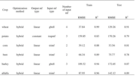
A hybrid intelligent system called ANFIS (the adaptive neuro-fuzzy inference system) for predicting VW was also applied. ANFIS was trained with the help of MATLAB 7.11.0 R2010b, and six top models, were selected based on RMSE, and R2. ANFIS parameter types for the six models and their values are presented in Table 4.

A multi-criteria assessment was conducted to evaluate the success of each model. The estimation capability of each model is evaluated using the Root Mean Square Error (R-MSE), and determination coefficient (R2) criteria. Formulas for calculating RMSE, and R2_{are given as follows:}

(12)

RMSE = 1

𝑛 (Oi− Pi

n

i=1

)2

(13) 𝑅2₌ 𝑛𝑖=1(𝑂𝑖− 𝑂 )(𝑃𝑖− 𝑃 )2

(𝑂𝑖− 𝑂 )2 𝑛𝑖=1(𝑃𝑖− 𝑃 )2 𝑛

𝑖=1

Where n is the number of observations,𝑖is the index for the number of data,Oi and Pi are the measured and predicted

values, respectively (Araghinejad and Burn, 2005).

4.

RESULTS AND DISCUSSIONS

Distribution of climatic elements such as temperature, precipitation, and wind velocity are affected by climatic factors such as altitude, longitude, latitude, slop. However, distribution of land and water, topography, and ocean currents as well as distribution of these climatic elements is very important in crop production (Lowry, 1972).

As mentioned earlier, different structures of the ANN models were employed for estimating VW in order to select the suitable parameter set combination of each model for each crop. The statistical measurements of the results obtained by each ANN models in training, validation and testing sets for different crops individually which are summarized in Table 2.

According to Table 2, the best number of neurons in hidden layer for MLP model and the best amount of spread (σ) for RBF and GRNN models are mentioned in column 3. The best percent of all data that were used for each set of training, validation, and testing ANN models have been shown in column 4. Column 7 shows the best network among the applied ANN models for each crop.

The obtained results show that RBF model with the smallest RMSE and the highest R2 was the best model for predicting VW content of corn, sugerbeet, and alfalfa. Furthermore, the value of spread for RBF model assigned to all crops was 0.5.

optimization method performed better than back propagation method for each crop. The linear mf was selected as better output mf for each crop except potato. In most crop (corn, sugerbeet, and alfalfa) the best input mf were trimf, and gbell mf was selected for wheat and barley, while trapmf was selected for potato. gaussmf and sigmf were not performed as the best mf for any crop. In potato was different from other crops in reference to output and input mf.

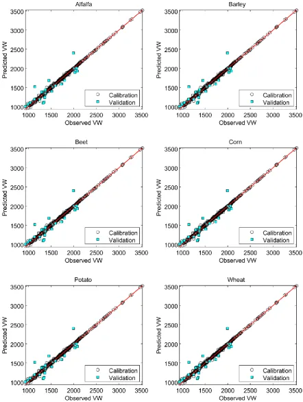
The coefficient of correlation between measured and predicted values is considered as a valuable indicator of the predictability of models. These relationships, presented in Figure 5, were found to be highly correlated. Cross-correlation between predicted and observed values (Figure 5) indicated that the constructed ANFIS model is acceptable for prediction of VW for each crop.

According to the RMSE and R2 values (Table 4), selected ANFIS model has a high prediction performance for estimation of VW for each crop. The same results were reported by Kisi and Ozturk (2007) for evapotranspiration

estimation and also Aali et al (2009) in estimation of saturation percentage of Soil.

5.

CONCLUSION REMARKS

In this study, VW volume of common crops in Iran was determined by CWR and crop yield. Three ANN structures (MLP, RBF, and GRNN) and ANFIS were applied in this regards. The comparison of obtained results according to RMSE and R2 showed that among the applied ANNs (MLP, RBF, and GRNN) structures, RBF with the least amount of RMSE equal to 80.88, 101.00, 48.88, 153.22 and highest R2 equal to 0.96, 0.92, 0.91, and 0.886 was found to be the most accurate model for estimating the VW of wheat, potato, corn, and barley, respectively. Although, the MLP was the best model, the other ANN models were suitable to estimate the VW volume. A comparison between the RBF and ANFIS showed that ANFIS with lower RMSE and higher R2 was more accurate for each crop.

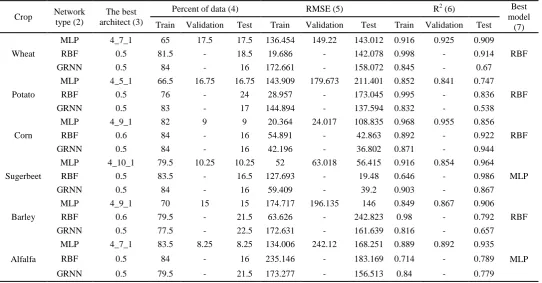
Table 2. Statistical analysis for the ANN models in training, validation, and testing sets

Crop Network type (2)

The best architect (3)

Percent of data (4) RMSE (5) R2 (6) Best

model (7) Train Validation Test Train Validation Test Train Validation Test

Wheat

MLP 4_7_1 65 17.5 17.5 136.454 149.22 143.012 0.916 0.925 0.909 RBF

RBF 0.5 81.5 - 18.5 19.686 - 142.078 0.998 - 0.914

GRNN 0.5 84 - 16 172.661 - 158.072 0.845 - 0.67

Potato

MLP 4_5_1 66.5 16.75 16.75 143.909 179.673 211.401 0.852 0.841 0.747 RBF

RBF 0.5 76 - 24 28.957 - 173.045 0.995 - 0.836

GRNN 0.5 83 - 17 144.894 - 137.594 0.832 - 0.538

Corn

MLP 4_9_1 82 9 9 20.364 24.017 108.835 0.968 0.955 0.856

RBF

RBF 0.6 84 - 16 54.891 - 42.863 0.892 - 0.922

GRNN 0.5 84 - 16 42.196 - 36.802 0.871 - 0.944

Sugerbeet

MLP 4_10_1 79.5 10.25 10.25 52 63.018 56.415 0.916 0.854 0.964

MLP

RBF 0.5 83.5 - 16.5 127.693 - 19.48 0.646 - 0.986

GRNN 0.5 84 - 16 59.409 - 39.2 0.903 - 0.867

Barley

MLP 4_9_1 70 15 15 174.717 196.135 146 0.849 0.867 0.906

RBF

RBF 0.6 79.5 - 21.5 63.626 - 242.823 0.98 - 0.792

GRNN 0.5 77.5 - 22.5 172.631 - 161.639 0.816 - 0.657

Alfalfa

MLP 4_7_1 83.5 8.25 8.25 134.006 242.12 168.251 0.889 0.892 0.935

MLP

RBF 0.5 84 - 16 235.146 - 183.169 0.714 - 0.789

Table 3. Preferred ANFIS’s parameter type and their performance indices

Crop Optimization method

Output mf type

Input mf type

Number of input

mf

Train Test

RMSE R2 RMSE R2

wheat hybrid linear gbell 4 37.84 0.99 129.26 0.91

potato hybrid constant trapmf 3 159.85 0.83 170.26 0.79

corn hybrid linear trimf 2 39.12 0.88 53.56 0.81

beet hybrid linear trimf 2 66.34 0.89 75.77 0.78

barley hybrid linear gbell 3 109.32 0.94 172.65 0.87

Table 4. Statistical analysis between preferred ANN and ANFIS models based on RMSE and R2

Crop ANFIS ANN

RMSE R2 RMSE R2

wheat 129.26 0.91 120.77 0.94

potato 170.26 0.79 151.38 0.84

corn 53.56 0.81 49.58 0.77

beet 75.77 0.78 127.69 0.65

barley 172.65 0.87 274.67 0.75

alfalfa 142.12 0.89 235.15 0.71

6.

REFERENCES

[1] Aali, K. A., Parsinejad, M., and Rahmani, B. 2009. Estimation of saturation percentage of soil using multiple regression, ANN, and ANFIS techniques. Computer and Information Science 2, P127.

[2] Alizadeh, A., and Keshavarz, A. 2005. Status of agricultural water use in Iran. In "Water Conservation, Reuse, and Recycling: Proceedings of an Iranian-American Workshop", pp. 94-105. National Academies Press.

[3] Allen, R. G., Pereira, L., Raes, D., and Smith, M. 1998a. FAO Irrigation and drainage paper No. 56. Rome: Food and Agriculture Organization of the United Nations, 26-40.

[4] Allen, R. G., Pereira, L. S., Raes, D., and Smith, M. 1998b. Crop evapotranspiration-Guidelines for computing crop water requirements-FAO Irrigation and drainage paper 56. FAO, Rome 300, 6541.

[5] Araghinejad, S., and Burn, D. H. 2005. Probabilistic forecasting of hydrological events using geostatistical analysis/Prévision probabiliste d'événements hydrologiques par analyse géostatistique. Hydrological sciences journal 50.

[6] Bouwer, H. 2000. Integrated water management: emerging issues and challenges. Agricultural water management 45, 217-228.

[7] Brown, S. C., Mason, C. A., Lombard, J. L., Martinez, F., Plater-Zyberk, E., Spokane, A. R., Newman, F. L., Pantin, H., and Szapocznik, J. 2009. The relationship of built environment to perceived social support and psychological distress in Hispanic elders: The role of “eyes on the street”. The Journals of Gerontology Series B: Psychological Sciences and Social Sciences 64, 234-246.

[8] Dietzenbacher, E., and Velázquez, E. 2007. Analysing Andalusian virtual water trade in an input–output framework. Regional Studies 41, 185-196.

[9] Drake, J. T. 2000. "Communications phase synchronization using the adaptive network fuzzy inference system (anfis)," New Mexico State University.

[10] Fang, S., Pei, H., Liu, Z., Beven, K., and Wei, Z. 2010. Water resources assessment and regional virtual water potential in the Turpan Basin, China. Water resources management 24, 3321-3332.

[11] Jang, J.-S. R., Sun, C.-T., and Mizutani, E. 1997. Neuro-fuzzy and soft computing-a computational approach to learning and machine intelligence [Book Review]. Automatic Control, IEEE Transactions on 42, 1482-1484.

[12] Kisi, O. 2007. Evapotranspiration modelling from climatic data using a neural computing technique. Hydrological Processes 21, 1925-1934.

[13] Laslett, G., McBratney, A., Pahl, P. J., and Hutchinson, M. 1987. Comparison of several spatial prediction methods for soil pH. Journal of Soil Science 38, 325-341.

[14] Lowry, W. P. 1972. "Compendium of lecture notes in climatology for Class III meteorological personnel," Secretariat of the World Meteorological Organization.

[15] Montazar, A., and Zadbagher, E. 2010. An analytical hierarchy model for assessing global water productivity of irrigation networks in Iran. Water resources management 24, 2817-2832.

[16] Shahlaei, M., Sabet, R., Ziari, M. B., Moeinifard, B., Fassihi, A., and Karbakhsh, R. 2010. QSAR study of anthranilic acid sulfonamides as inhibitors of methionine aminopeptidase-2 using LS-SVM and GRNN based on principal components. European journal of medicinal chemistry 45, 4499-4508.

[17] Wang, Y.-m., Chang, J.-x., and Huang, Q. 2010. Simulation with RBF neural network model for reservoir operation rules. Water resources management 24, 2597-2610.