RADAR
Research Archive and Digital Asset Repository
Ibarguren-Arrieta, I., Perez, J., Muguerza, J., Rodriguez, D. and Harrison, R. () 'The Consolidated Tree Construction
Algorithm in Imbalanced Defect Prediction Datasets'. . Congress on Evolutionary Computation, San Sebastian
DOI:
This document is the authors’ Accepted Manuscript.
License:
https://creativecommons.org/licenses/by-nc-nd/4.0
Available from RADAR:
https://radar.brookes.ac.uk/radar/items/3f8a3534-afca-4cb2-b577-be06f2381324/1/
Copyright © and Moral Rights are retained by the author(s) and/ or other copyright owners unless otherwise waved in
a license stated or linked to above. A copy can be downloaded for personal non-commercial research or study, without
prior permission or charge. This item cannot be reproduced or quoted extensively from without first obtaining
permission in writing from the copyright holder(s). The content must not be changed in any way or sold commercially
in any format or medium without the formal permission of the copyright holders.
The Consolidated Tree Construction Algorithm in
Imbalanced Defect Prediction Datasets
Igor Ibarguren
∗, Jes´us M. P´erez
∗, Javier Mugerza
∗, Daniel Rodriguez
§, Rachel Harrison
¶∗Dept of Computer Science Univ of the Basque Country
20018 Donostia, Spain
Email:{igor.ibarguren, txus.perez, javier.mugerza}@ehu.eus §University of Alcala
28871 Alcal´a de Henares, Madrid, Spain Email:[email protected]
¶School of Technology Oxford OX33 1HX, UK
Email: [email protected]
Abstract—In this short paper, we compare well-known rule/tree classifiers in software defect prediction with the CTC decision tree classifier designed to deal with class imbalance. It is well-known that most software defect prediction datasets are highly imbalance (non-defective instances outnumber defective ones). In this work, we focused only on tree/rule classifiers as these are capable of explaining the decision, i.e., describing the metrics and thresholds that make a module error prone. Furthermore, rules/decision trees provide the advantage that they are easily understood and applied by project managers and quality assurance personnel. The CTC algorithm was designed to cope with class imbalance and noise datasets instead of using preprocessing techniques (oversampling or undersampling), ensembles or cost weights of misclassification. The experimental work was carried out using the NASA datasets and results showed that induced CTC decision trees performed better or similar to the rest of the rule/tree classifiers.
I. INTRODUCTION
The imbalance problem is an important topic of research in supervised classification where the number of instances of a class outnumbers the others. When dealing with imbalanced datasets, there are different approaches: (i) preprocessing tech-niques to balance the number of instances across the labels, (i) cost-sensitive approaches to penalise differently the types of errors, (iii) ensembles of classifiers to make them robust to the imbalance problem, (iv) hybrid techniques combining previous approaches, or finally, making the algorithms more robust to the imbalance problem. For recent recent surveys, we refer to the the works by Branco et al. [1] and Haixiang et al. [2]).
In this work, we address the problem of software defect prediction (SDP) as an important area of research in Software Engineering. In SDP most datasets are highly imbalanced (the number of defective modules highly outnumbers the non-defective ones) with an algorithm that it is robust to the imbalance problem, the CTC algorithm developed by P´erez et al. [3]. There are multiple papers on using a variety of machine learning techniques in software defect prediction. However, the use of tree or rule classifiers helps explaining
why modules can be defect prone. These classifiers select the software metrics and assign thresholds to them in an intuitive and easily applicable way. Therefore, we compare the most popular tree or rule classification algorithms using well-known NASA datasets (the version curated by Shepperd et al. [4] and named D’) with the CTC algorithm.
The rest of the paper is organised as follows. Next, Sec-tion II overviews previous work in this field. This is followed by Section III, that describes briefly the experimental work which is composed of a description of datasets used, evaluation measures, and a brief statistical analysis of the results. Finally, Section IV concludes the paper and outlines future work.
II. PREVIOUSWORK
Fern´andez et al. [5] proposed a taxonomy of genetics-based machine algorithms for rule induction, classifying 16 algorithms into three categories based on the chromosome codification. One of the categories was further divided into three subcategories based on their approach for a total of five subcategories. They performed a hierarchical analysis of the performance of these algorithms over 96 datasets divided into three contexts. Two of these contexts had a high degree of imbalance, whereas the third context was a balanced version of the second. First, an intra-subcategory analysis was performed. Then, the winners of each subcategory were compared to six non-evolutionary algorithms. In one of the classification con-texts (two-class non-preprocessed imbalanced classification), Ripper (a non-evolutionary rule-induction algorithm) placed first. The only evolutionary algorithms without statistically significant differences with RIPPER were Oblique-DT and GAssist (placing 3rd and 5th, respectively).
A later work by Ibarguren et al. [6] extended these experi-ments by adding CTC to the study. In this case CTC performed best for two-class non-resampled dataset classification, per-forming significantly better than GAssist (now placing 6th). These results led us to believe that CTC could perform well in the context of software defect prediction as these datasets
TABLE I
MDP NASA DATASETSDESCRIPTION
# Instances D’ %Imbalance Ratio # Attributes
CM1 344 12.21 41 JM1 9,593 18.34 22 KC1 2,095 15.51 22 KC3 200 18 41 MC1 8,737 0.78 40 MC2 127 34.65 41 MW1 264 10.23 41 PC1 759 8.04 41 PC2 1,493 1.07 41 PC3 1,125 12.44 41 PC4 1,399 12.72 41 PC5 16,962 2.96 40
are imbalanced and the comprehensibility of the classification (provided by the single tree CTC creates) is important.
From the software defect prediction point of view, there is a vast amount of work applying numerous machine learning techniques and comprehensive surveys include the ones by Hall et al. [7] and Catal [8]. Most works focused on comparing and analysing machine learning algorithms (e.g. [9])and pre-processing techniques such as feature selection. More recent works focuses on problems such as noise and imbalance [10], [12].
The different approaches to deal with imbalanced can be classified into data as sampling, cost-sensitive, ensemble ap-proaches or hybrid apap-proaches [11]. In this work, we compare only rule or tree classifiers taking into account the imbalance nature of software defect datasets. In addition, rule or tree classifiers can explain why a software module is error prone providing the metrics and thresholds for those metrics. Rules are also easily understood and applied by project managers and quality assurance personnel in contrast to black box algorithms such as neural networks or ensembles.
III. EXPERIMENTALWORK
A. Datasets
We have carried out the experimental work using available software defect prediction datasets generated from NASA projects. In particular, we have used curated datasets by Shepperd et al. [4] who analysed different problems with these datasets and available in the Promise Repository1. Although
some quality issues have been reported by Shepperd et al. [4], and by Bowes et al. [13], [14] these datasets are the most popular ones in defect prediction and it allows us to compare our results with the literature.
Table I shows the number of instances for each dataset, their imbalance ratio (IR) and number of attributes. All datasets contain attributes mainly composed of different McCabe [15], Halstead [16] and count metrics. The last boolean attribute represents whether the class is (defective).
These sets of metrics (both McCabe and Halstead) have been used for QA during development, testing and mainte-nance. Generally, the developers or maintainers use threshold
1http://openscience.us/repo/
TABLE II
CONFUSIONMATRIX FORTWOCLASSES Act
Pos Neg
Pred
Pos True Pos (T P) False Pos (F P) (False alarm) P P V= Conf= P rec= T P T P+F P Neg False Neg
(F N) True Neg (T N) N P V = T N F N+T N Recall= Sens= T Pr= T P T P+F N Spec= T Nr= T N F P+T N
values. For example, if the cyclomatic complexity (v(g)) of a module is between 1 and 10, it is considered to have a very low risk of being defective; however, any value greater than 50 is considered to have an unmanageable complexity and risk. Although these metrics have been used for long time, there are no generally agreed thresholds.
It can be observed that most datasets are highly imbalanced, varying their IR from less than 1% to 30% and there are large numbers of duplicates and inconsistencies in some of the datasets. We used the cleaned version with dupicates (D’) as there is no reason to remove them if they are the real distribution. This however can lead to optimistic results since the same instances can be in both training and testing datasets. However, there are many other factors affecting the performance of the classifiers, for example, the degree of data overlapping among the classes is another factor that lead to the decrease in performance of learning algorithms. As stated by L´opez et al. [17] there are other problems: dataset shift (training and test data follow different distributions), distribution of the cross validation data, small disjuncts, the lack of density or small sample size, the class overlapping, the correct management of borderline examples or noisy data. B. Evaluation Measures
In the case of binary classifiers, many of the performance measures can be obtained from the confusion matrix (Table II). There is a trade-off between thetrue positive rate andtrue negative rateas the objective is to maximise both metrics. A classical evaluation technique to consider this trade-off when data is imbalanced is the Receiver Operating Characteristic (ROC) [18] curve which provides a graphical visualisation of the results. This graphical representation can be summarised as the Area Under the ROC Curve (AUC) providing a quality measure between positive and negative rates with a single value. Its range goes from 0 to 1 (the closer to one the better and 0.5 is equivalent to a random classification).
Another suitable and interesting performance metric for binary classification when data are imbalanced is Matthew’s Correlation Coefficient (M CC) [19]. Its range goes from -1 to +-1; the closer to one the better as it indicates perfect prediction whereas a value of 0 means that classification is not better than random prediction and negative values mean that predictions are worse than random.
M CC= p T P ×T N−F P ×F N
(T P+F P)(T P +F N)(T N+F P)(T N+F N)
(1) C. Rule Classifiers
In this work, we compare CTC [3], against other classi-fiers. The CTC (Consolidated Tree Construction) algorithm was created for an insurance fraud detection problem where class imbalance was present. CTC creates a set of balanced subsamples from a training sample, and, in contrast to other multiple classifier systems, it builds a single decision tree understandable by humans. The method is based on the well-known C4.5 algorithm. The CTC algorithm uses a voting pro-cess to decide the variable that will split the node at each step of the tree’s building process based on the decisions proposed by C4.5 algorithm in each subsample. An implementation of the CTC algorithm for Weka, called J48Consolidated, can be found in the Web2.
The comparison is performed against popular tree/rule classifiers all implemented in Weka, and using their default parameters:
• C4.5 [20] (J48 in Weka) is a decision tree. Decision trees are constructed in a top-down approach. The leaves of the tree correspond to classes, nodes correspond to features, and branches to their associated values. To classify a new instance, one simply examines the features tested at the nodes of the tree and follows the branches corresponding to their observed values in the instance.
• RIPPER (Repeated Incremental Pruning to Produce Error Reduction) is a rule based classifier [21], [22]. The algorithm is composed of three stages in which set of rules are induced using the information gain ratio as a measure, pruned used information gain and optimised respectively.
• CART (Classification and Regression Trees) [23] algo-rithm induces multiple decision trees. Each node of the decision trees starting from the root is a two branch bifurcation of the most discriminating attribute based on the Gini index. Induced trees are later pruned instead of employing a stopping criterion. The CART algorithm is more complex and time consuming than C4.5’s since multiple trees need to be built and pruned, but trees are generally simpler [24].
• PART [25] is an algorithm, which was designed by the authors of the Weka platform, that builds a rule set. The aim was to achieve the combination of the capacities of two algorithms: C4.5 and RIPPER. C4.5 is used to build a partial decision tree that will be used to extract one rule. The examples not covered by this rule are used to generate a new sample in order to build the next partial tree. The process is repeated until the remaining sample is assigned to the root node.
2http://www.aldapa.eus/res/weka-ctc/
TABLE III D’ RESULTS USINGAUC
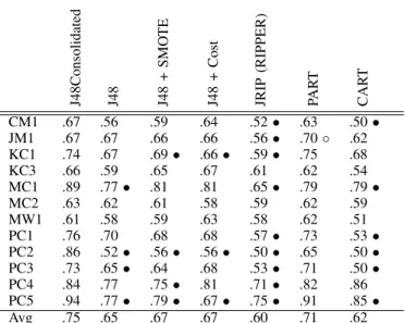
J48Consolidated J48 J48 + SMO TE J48 + Cost JRIP (RIPPER) P AR T CAR T CM1 .67 .56 .59 .64 .52• .63 .50• JM1 .67 .67 .66 .66 .56• .70◦ .62 KC1 .74 .67 .69• .66• .59• .75 .68 KC3 .66 .59 .65 .67 .61 .62 .54 MC1 .89 .77• .81 .81 .65• .79 .79• MC2 .63 .62 .61 .58 .59 .62 .59 MW1 .61 .58 .59 .63 .58 .62 .51 PC1 .76 .70 .68 .68 .57• .73 .53• PC2 .86 .52• .56• .56• .50• .65 .50• PC3 .73 .65• .64 .68 .53• .71 .50• PC4 .84 .77 .75• .81 .71• .82 .86 PC5 .94 .77• .79• .67• .75• .91 .85• Avg .75 .65 .67 .67 .60 .71 .62
◦,•statistically significant improvement or degradation
In addition we have also used J48 with filters to deal with imbalance. In particular, we have used (i) SMOTE (Synthetic Minority Over-sampling Technique) [26] a popular sampling technique which increases the number of the minority in-stances based on their neighbours, and (ii) cost sensitive classification in which a matrix cost penalises classification errors.
D. Empirical Results
We have generated multiple results for all the techniques and metrics previously mentioned using Weka’s Experimenter using 5 times 5 Cross Validation (5x5CV) over all algorithms and datasets. We next present the most relevant results together with a discussion leaving other material on the companion Web site.
Tables III and IV show the results of using as base learner the C4.5 algorithm (called J48 in Weka) with the default parameters (using pruning, with the minimum number of instances per leaf as two and no Laplace smoothing). The first numerical column shows the results for the base classifier and the rest of the columns show the results of the different algorithms and whether they are statistically significant using thet-test at 0.05 significance level. These results were obtained with Weka’s experimenter tool.
We have used the t-test to statistically compare the per-formance of the different classifiers with the CTC classifier using MCC and AUC. The t-test is provided by Weka’s Ex-perimenter. We have also compared the classifiers using non-parametric tests as recommended in recent literature (e.g. [27], [28], [29]) using the KEEL tool [30]3. In fact, we use the
Friedman Aligned Ranks test to discover whether or not there are significant differences between the algorithms. This test
TABLE IV D’ RESULTS USINGMCC J48Consolidated J48 J48 + SMO TE J48 + Cost JRIP (RIPPER) P AR T CAR T CM1 .24 .10 .17 .23 .05 .09 .00• JM1 .27 .23• .24 .24 .20• .17• .17• KC1 .34 .28 .31 .32 .26 .24• .21• KC3 .25 .22 .29 .24 .26 .23 .11 MC1 .19 .44◦ .43◦ .44◦ .42◦ .44◦ .44◦ MC2 .25 .21 .20 .16 .23 .26 .22 MW1 .14 .32 .15 .20 .19 .28 .00 PC1 .28 .24 .26 .30 .25 .23 .08• PC2 .18 .00• .09 .09 .01• .07 .00• PC3 .33 .24 .22 .29 .10• .14• .00• PC4 .51 .51 .52 .51 .44 .46 .40• PC5 .49 .50 .54◦ .52 .51 .42 .44 Avg .29 .27 .29 .29 .24 .25 .17 ◦,•statistically significant improvement or degradation
ranks the algorithms taking into account a weighted system, in which the harder to classify the data set is, the larger is the weight. On the other hand, when significant differences were found, the post-hoc 1xN Holm procedure was used in order to analyze which pairs of algorithms had statistical differences using the CTC as the control algorithm.
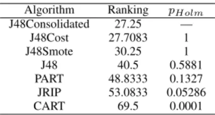
The average ranks obtained by each algorithm in the Fried-man Aligned test, as well as, the adjusted p-values computed using Holm post-hoc test are shown in Tables V and VI using MCC and AUC performance measures respectively. As it can be observed, CTC (J48Consolidated) ranks first for both performance measures, obtaining statistically significant differ-ences in both cases based on Friedman Aligned Ranks test (at 0.05 significance level). In the first positions of the rankings, for the both measures, we can found the used variants of C4.5 (J48), with the exception of the PART algorithm which achieves the second rank using the AUC measure (the PART algorithm is a combination of C4.5 and Ripper).
Regarding the results of the Holm test, the results are qualitatively different for MCC and AUC. In the case of MCC values, CTC only achieves statistically significant differences when comparing with CART. However, in the case of AUC, significant differences were found with all algorithms except with PART. It is worth noting that the ROC curve represents multiple pairs of T P rate and F P rates while changing the decision threshold of an example to belong to a class. Thus, the Area Under ROC curve (AUC) evaluates the classifier in multiple contexts of the classification space and because of this is considered a robust performance metric and is widely used in the community.
IV. CONCLUSIONS ANDFUTUREWORK
In this paper, we compared different tree/rule classifiers and evaluation metrics in the domain of software defect prediction
TABLE V
MCC AVERAGERANKINGS OF THE ALGORITHMS(ALIGNEDFRIEDMAN) AND AJUSTED P-VALUE(HOLM TEST)
Algorithm Ranking pHolm
J48Consolidated 27.25 — J48Cost 27.7083 1 J48Smote 30.25 1 J48 40.5 0.5881 PART 48.8333 0.1327 JRIP 53.0833 0.05286 CART 69.5 0.0001 TABLE VI
AUC AVERAGERANKINGS OF THE ALGORITHMS(ALIGNEDFRIEDMAN) AND AJUSTED P-VALUE(HOLM TEST)
Algorithm Ranking pHolm
J48Consolidated 13.7083 — PART 21.625 0.4266 J48Cost 39.2083 0.0208 J48Smote 44.4167 0.0061 J48 50.3333 0.0009 CART 58.4167 0 JRIP 69.7917 0
using datasets originated by NASA projects which have been cleaned and preprocessed by Shepperd et al. In particular, we compared the CTC (Consolidated Tree Construction algo-rithm) with other well-known algorithms using both the AUC and MCC measures. The CTC algorithm dealt well with these datasets which have a high level of imbalance and problematic instances (noise) based on the results of parametric and non-parametric statistical tests.
Future work could, on the one hand, include other consol-idated algorithms into this study. Until recently research on consolidation has focused on decision trees. However, rule-induction algorithms such as PART and RIPPER are expected to be consolidated in the near future. More class imbalance-oriented resampling techniques such as SMOTE+ENN or EUSCHC [31] could be added to the study and applied to the rest of algorithms other than J48. It could also be interesting to compare these algorithms with available WEKA imple-mentations of evolutionary algorithms, if any, and ensemble algorithms specifically tailored to tackle class imbalance [32]. However, it should be noted that these ensemble algorithms lack the ability to produce comprehensible classifiers.
On the other hand, a further study could look into the effect of different dataset characteristics such as size, imbalance ratio and attribute number on the performance, complexity and scalability of the classifiers used in this study. The datasets could be analysed using the measures proposed by Orriols-Puig [33] and the performance of the classifiers evaluated accordingly.
Finally, this study could be extended by adding more datasets and analysing the simplicity and applicability of the rules induced by the algorithms.
ACKNOWLEDGEMENTS
This research has been partially supported by the De-partment of Education, Universities and Research (Schol-arship PRE-2013-1-887, BOPV/2013/128/3067) and by the Department of Economic Development and Competitiveness (ADIAN, grant IT-980-16) of the Basque Government; and by the Ministry of Economy and Competitiveness of the Spanish Government and by the European Regional Development Fund - ERDF (eGovernAbility, grant TIN2014-52665-C2-1-R, MINECO/FEDER) and by European Commission funding under the 7th FP IAPP Marie Curie program for project (ICEBERG, grant 324356).
REFERENCES
[1] P. Branco, L. Torgo, and R. P. Ribeiro, “A survey of predictive modeling on imbalanced domains,” ACM Computuing Surveys, vol. 49, no. 2, pp. 31:1–31:50, Aug. 2016. [Online]. Available: http://doi.acm.org/10.1145/2907070
[2] G. Haixiang, L. Yijing, J. Shang, G. Mingyun, H. Yuanyue, and G. Bing, “Learning from class-imbalanced data: Review of methods and applications,”Expert Systems with Applications, 2016.
[3] J. M. P´erez, J. Muguerza, O. Arbelaitz, I. Gurrutxaga, and J. I. Mart´ın, “Combining multiple class distribution modified subsamples in a single tree,” Pattern Recognition Letters, vol. 28, no. 4, pp. 414–422, Mar. 2007. [Online]. Available: http://www.sciencedirect.com/science/article/ pii/S0167865506002285
[4] M. Shepperd, Q. Song, Z. Sun, and C. Mair, “Data quality: Some comments on the nasa software defect datasets,”IEEE Transactions on
Software Engineering, vol. 39, no. 9, pp. 1208–1215, 2013.
[5] A. Fern´andez, S. Garcia, J. Luengo, E. Bernad´o-Mansilla, and F. Herrera, “Genetics-based machine learning for rule induction: State of the art, taxonomy, and comparative study,” Evolutionary Computation, IEEE
Transactions on, vol. 14, no. 6, pp. 913–941, 2010.
[6] I. Ibarguren, J. M. P´erez, J. Muguerza, I. Gurrutxaga, and O. Arbelaitz, “Coverage based resampling: Building robust consolidated decision trees,”Knowledge-Based Systems, vol. 79, pp. 51 – 67, 2015. [7] T. Hall, S. Beecham, D. Bowes, D. Gray, and S. Counsell, “A
systematic literature review on fault prediction performance in software engineering,” vol. 38, no. 6, pp. 1276–1304, 2012. [Online]. Available: http://ulir.ul.ie/handle/10344/1772
[8] C. Catal, “Software fault prediction: A literature review and current trends,”Expert Systems with Applications, vol. 38, no. 4, pp. 4626 – 4636, 2011. [Online]. Available: http://www.sciencedirect.com/science/ article/pii/S0957417410011681
[9] S. Lessmann, B. Baesens, C. Mues, and S. Pietsch, “Benchmarking classification models for software defect prediction: A proposed frame-work and novel findings,”IEEE Transactions on Software Engineering, vol. 34, no. 4, pp. 485–496, July-Aug. 2008.
[10] S. Wang and X. Yao, “Using class imbalance learning for software defect prediction,”IEEE Transactions on Reliability, vol. 62, no. 2, pp. 434– 443, June 2013.
[11] D. Rodriguez, I. Herraiz, R. Harrison, J. Dolado, and J. C. Riquelme, “Preliminary comparison of techniques for dealing with imbalance in software defect prediction,” inProceedings of the 18th International Conference on Evaluation and Assessment in Software Engineering
)EASE=, ser. EASE’14. New York, NY, USA: ACM, 2014, pp. 43:1–
43:10. [Online]. Available: http://doi.acm.org/10.1145/2601248.2601294 [12] C. Seiffert, T. Khoshgoftaar, and J. Van Hulse, “Improving software-quality predictions with data sampling and boosting,”IEEE Transactions
on Systems, Man and Cybernetics, Part A: Systems and Humans, vol. 39,
no. 6, pp. 1283–1294, 2009.
[13] D. Bowes, T. Hall, and D. Gray, “DConfusion: a technique to allow cross study performance evaluation of fault prediction studies,”Automated
Software Engineering, vol. 21, no. 2, pp. 287–313, Jul. 2013. [Online].
Available: http://link.springer.com/10.1007/s10515-013-0129-8
[14] D. Gray, D. Bowes, N. Davey, and B. Christianson, “The misuse of the NASA Metrics Data Program data sets for automated software defect prediction,” in 15th Annual Conference on Evaluation & Assessment
in Software Engineering (EASE 2011). IET, Jan. 2011, pp. 96–103.
[Online]. Available: http://digital-library.theiet.org/content/conferences/ 10.1049/ic.2011.0012
[15] T. McCabe, “A complexity measure,”IEEE Transactions on Software
Engineering, vol. 2, no. 4, pp. 308–320, December 1976.
[16] M. Halstead, Elements of software science, ser. Elsevier Computer Science Library. Operating And Programming Systems Series; 2. New York ; Oxford: Elsevier, 1977.
[17] V. L´opez, A. Fern´andez, and F. Herrera, “On the importance of the validation technique for classification with imbalanced datasets: Addressing covariate shift when data is skewed,” Information
Sciences, vol. 257, pp. 1–13, 2014. [Online]. Available: http:
//www.sciencedirect.com/science/article/pii/S0020025513006804 [18] T. Fawcett, “An introduction to roc analysis,” Pattern Recogn.
Lett., vol. 27, no. 8, pp. 861–874, Jun. 2006. [Online]. Available:
http://dx.doi.org/10.1016/j.patrec.2005.10.010
[19] B. W. Matthews, “Comparison of the predicted and observed secondary structure of t4 phage lysozyme,” Biochimica et biophysica acta, vol. 405, no. 2, pp. 442–451, Oct. 1975. [Online]. Available: http://view.ncbi.nlm.nih.gov/pubmed/1180967
[20] J. Quinlan, C4.5: Programs for machine learning. San Mateo, California: Morgan Kaufmann, 1993.
[21] W. W. Cohen and Y. Singer, “A simple, fast, and effective rule learner,”
in Proceedings of the National Conference on Artificial Intelligence.
John Wiley & Sons, 1999, pp. 335–342.
[22] W. W. Cohen, “Fast effective rule induction,” inTwelfth International
Conference on Machine Learning. Morgan Kaufmann, 1995, pp. 115–
123.
[23] L. Breiman, J. H. Friedman, R. A. Olshen, and C. J. Stone,Classification
and Regression Trees. Belmont, California: Wadsworth International
Group, 1984.
[24] T. Oates and D. Jensen, “The effects of training set size on decision tree complexity,” inProceedings of the Fourteenth International Conference
on Machine Learning (ICML). Citeseer, 1997, pp. 254–262.
[25] E. Frank and I. H. Witten, “Generating accurate rule sets without global optimization,” in Proceedings of the Fifteenth International
Conference on Machine Learning, ser. ICML ’98. San Francisco, CA,
USA: Morgan Kaufmann Publishers Inc., 1998, pp. 144–151. [Online]. Available: http://dl.acm.org/citation.cfm?id=645527.657305
[26] N. V. Chawla, K. W. Bowyer, L. O. Hall, and W. P. Kegelmeyer, “Smote: Synthetic minority over-sampling technique,”J. Artif. Intell. Res. (JAIR), vol. 16, pp. 321–357, 2002.
[27] J. Demˇsar, “Statistical comparisons of classifiers over multiple data sets,”
Journal of Machine Learning Research, vol. 7, pp. 1–30, Dec. 2006.
[Online]. Available: http://dl.acm.org/citation.cfm?id=1248547.1248548 [28] S. Garc´ıa and F. Herrera, “An extension on ”statistical comparisons of classifiers over multiple data sets” for all pairwise comparisons,”Journal
of Machine Learning Research, vol. 9, pp. 2677–2694, 2009. [Online].
Available: http://www.jmlr.org/papers/volume9/garcia08a/garcia08a.pdf [29] S. Garc´ıa, A. Fern´andez, J. Luengo, and F. Herrera, “Advanced
non-parametric tests for multiple comparisons in the design of experiments in computational intelligence and data mining: Experimental analysis of power,”Inf. Sci., vol. 180, pp. 2044–2064, 2010.
[30] J. Alcal´a-Fdez, L. S´anchez, S. Garc´ıa, M. J. Jesus, S. Ventura, J. M. Garrell, J. Otero, C. Romero, J. Bacardit, V. M. Rivas, J. C. Fern´andez, and F. Herrera, “KEEL: a software tool to assess evolutionary algorithms for data mining problems,” Soft Computing, vol. 13, no. 3, pp. 307–318, May 2008. [Online]. Available: http://link.springer.com/10.1007/s00500-008-0323-y
[31] S. Garca and F. Herrera, “Evolutionary undersampling for classifica-tion with imbalanced datasets: Proposals and taxonomy,”Evolutionary
Computation, vol. 17, no. 3, pp. 275–306, Sep. 2009.
[32] M. Galar, A. Fernndez, E. Barrenechea, H. Bustince, and F. Herrera, “A review on ensembles for the class imbalance problem: Bagging-, boosting-, and hybrid-based approaches,”Systems, Man, and
Cybernet-ics, Part C: Applications and Reviews, IEEE Transactions on, vol. 42,
no. 4, pp. 463–484, 2012.
[33] A. Orriols-Puig, “New challenged in learning classifier systems: Mining rarities and evolving fuzzy models,” Ph.D. dissertation, Universitat Ramon Llull, Barcelona, Catalonia, Spain, 2008.