Munich Personal RePEc Archive
Lower bounds of concentration in a small
open economy
Ilmakunnas, Pekka
HECER
September 2006
öMmföäflsäafaäsflassflassflas
ffffffffffffffffffffffffffffffffffff
Discussion Papers
Lower Bounds of Concentration in
a Small Open Economy
Pekka Ilmakunnas
Helsinki School of Economics and HECER
Discussion Paper No. 118 September 2006
ISSN 1795-0562
HECER
Discussion Paper No. 118
Lower Bounds of Concentration in a Small Open
Economy*
Abstract
We examine how Sutton’s “bounds” approach works in a small country where industries have relatively high export and import intensities. Import competition is used as an indicator for the degree of competition in the low sunk cost industries. The bounds are estimated as stochastic frontiers, where observable industry characteristics, export intensity and entry barriers, are allowed to affect the mean and variance of the deviations from the frontier. In accordance with the theory, high R&D intensity industries have a lower bound for concentration, which is higher than that for low sunk cost intensity industries. For high advertising industries the theory does not hold as well. High import competition leads to a higher bound in the low sunk cost industries.
JEL Classification: L11, L13, L60
Keywords: Concentration, sunk costs, R&D, stochastic frontiers
Pekka Ilmakunnas
Department of Economics Helsinki School of Economics P.O. Box 1210
FI-00101 Helsinki FINLAND
e-mail:[email protected]
1. Introduction
During the heyday of the structure-conduct-performance (SCP) paradigm there was much
research on the measurement of concentration and development of concentration
measures. Concentration was also analyzed in the open economy context by adjusting
concentration ratios for exports and imports or by explaining domestic concentration by
export and import intensity. The analysis of market structure has gained new interest
since the 1990s. One major factor behind this has been the research of Sutton (1991,
1998, 2006). He has developed theories on what determines a lower bound for
concentration. The emphasis in empirical work is then not in explaining the actual level
of concentration in different industries, but rather on testing whether different kinds of
industries have different lower bounds for their concentration levels. The emphasis is on
how endogenous sunk costs in the form of advertising or R&D lead to a lower bound for
concentration that is higher than the bound in industries without such sunk costs. With a
few exceptions (Lyons and Matraves, 1996, Lyons, Matraves, and Moffatt, 2001) the
bounds approach has not been discussed in an open economy context.
This paper has two purposes. First of all, we want to examine how well the predictions of
the “bounds” theory hold in a small open economy. It is not immediately clear that they
should hold, since many relevant markets are not national, but rather international.
Further, in a small country most industries have a fairly small number of firms and high
concentration. However, if the results are consistent with the bounds theory, they actually
give strong support for it as it since predicts well even in these “unfavorable” conditions.
In particular, we take into account the open economy aspect by defining the degree of
competition in industries based on the role of imports. Our second goal is to examine
whether industries deviate from the lower bound in such a systematic manner that can be
explained by variables that describe for example the entry conditions of the industries.
This is done by estimating the bound as a stochastic frontier, where various variables,
including export intensity and measures of entry barriers, affect the mean and variance of
a truncated error term. Hence deviations from the bound are treated like “inefficiencies”
approach and the older approach where concentration was directly explained by different
characteristics of the industries. The data that we use is from Finnish manufacturing.
Our results support the “bounds” approach as far as R&D is concerned, but for
advertising the results are less conclusive. It also appears that import intensity can be
regarded as a measure of the degree of competition in low sunk cost industries. The
results are relatively robust to different definitions of R&D intensity and to alternative
measures of concentration. We also find that systematic deviations from the lower bound
can be explained by observable industry characteristics.
The structure of the paper is as follows. In section 2 we briefly review earlier empirical
research on Sutton’s endogenous sunk costs model. In section 3 we present the data and
econometric approach to be used and in section 4 we report the estimation results.
Section 5 concludes the paper.
2. Previous research on the endogenous sunk costs model
Although theory does not give straightforward guidelines on the relationship between the
number of firms and degree of competition, some limits to their connection can be stated
(Sutton, 1991, 2002). The number of firms affects the level of the price negatively in all
market structures, except for the extreme cases of perfect collusion and homogeneous
goods Bertrand competition. On the other hand, given the market size, the more firms
there are, the smaller is the scale of production and the higher the price has to be for the
firms to survive. If the market size grows, it can accommodate more firms. These
relationships determine an inverse relationship between market size and the inverse of the
maximum possible number of firms, i.e. the lower bound for concentration. If all N firms
in an industry were of equal size, market structure could be measured with the number of
firms. The lower bound is an inverse relationship between market size and 1/N, which in
this equal firm size case equals the Herfindahl index H. If firm sizes vary, the bound, now
an inverse relationship between a concentration measure and market size is at some
concentration-market size space depends on the history of the industries, random events,
etc.
An essential feature of the bounds approach is the incorporation of endogenous sunk
costs in the determination of market structure. These include advertising and research and
development expenses. On one hand, they increase the customers’ willingness to pay for
the product, but on the other hand, they increase costs and raise the price required for
firm survival. As a result, the first prediction of the theory is that the lower bound of
concentration has to be at a higher level and industries with this kind of sunk costs tend to
be more concentrated. The second prediction is that when market size grows, the firms
may invest even more in sunk costs and concentration may decrease only slowly, and the
lower bound is less steep than in low sunk cost industries. In the industries with no sunk
costs increasing degree of price competition shifts the bound up (given market size),
since the number of firms has to fall for the firms to survive. This is the third prediction
of the theory.
In practice, the bound is estimated by regressing a measure of concentration on market
size. The concentration measure most typically used is logit transformation of a
concentration ratio, ln(C/(1-C)), but also logit transformation of Herfindahl index has
been used (Lyons and Matraves, 1996), or an untransformed concentration ratio. The
explanatory variable is usually some measure of market size relative to setup costs, S/σ.
To obtain a suitable convex form for the bound, this variable often enters in the form
1/ln(S/σ).
The definition of sunk cost industries varies somewhat in the literature. The empirical
work in Sutton (1991) considered only advertising, but the approach has been applied by
subsequent writers to both advertising and R&D (Robinson and Chiang, 1996, Lyons and
Matraves, 1996, Symeonidis, 2000, Lyons, Matraves, and Moffatt, 2001, Giorgetti,
2003).1 Industries can be divided to two types: 1: industries with no endogenous sunk
1 Sutton (1998) derives a lower bound relationship between concentration and market segmentation,
costs, and 2: endogenous sunk cost industries. Group 2 can be further divided to 2A:
advertising intensive industries, 2R: R&D intensive industries, and 2AR: both advertising
and R&D intensive industries. Given the market size, the lower bound for concentration
should be lowest in group 1; in group 2 it is higher and does not necessarily decrease
monotonically with market size. Various authors have used slightly different
combinations of these industry groups. Type 1 industries can further be divided to high
and low competition industries. We will use import intensity variables to measure the
degree of competition in these industries.
To test the hypothesis, one can pool all industries in estimation and include separate
intercepts for each industry type. Lyons and Matraves (1996) include the level of
integration in the equation for the bound, estimated using EU-level concentration and
market size data. This is based on the argument that the degree of integration of markets
should theoretically have an influence on the level of the bounds; this influence can be
different in the different types of industries. Lyons, Matraves, and Moffatt (2001) use a
switching regression model to determine whether the appropriate market is national or
EU market. Symeonidis (2000) includes a dummy variable describing the competition
regime, influenced by changes in cartel policy. Robinson and Chiang (1996) use separate
estimations for industries with different types of competition. Sometimes also the slope
coefficients are allowed to vary by industry type to test the second prediction.
Sutton (1991) estimated the model using a method that imposed the constraint that all
observations are above the boundary. Since the model includes two parameters, constant
and the coefficient of 1/ln(S/σ), the boundary goes through two observation points. This
method was used also by Robinson and Chiang (1996) and Marin and Siotis (2002), and
Giorgetti (2003) compares this method and quantile regression. A stochastic frontier has
been estimated by Lyons and Matraves (1996), and Marin and Siotis (2002). The
stochastic frontier approach allows industries to be in disequilibrium, i.e. it is possible
that they are occasionally situated below the theoretical (equilibrium) lower bound. An
average frontier (i.e., OLS estimation) has been used by Symeonides (2000), who found
that the errors had a wrong skew to be based on a stochastic frontier, and by Lyons,
Matraves, and Moffatt (2001), among others.
The traditional SCP way of examining the determinants of concentration was to include
several variables together in a regression model for concentration (see e.g. Davies, 1989).
These variables typically included advertising intensity and/or R&D intensity, measures
of barriers to entry, and often also export and import shares. In the bounds approach the
model is estimated separately for different types of industries without including R&D or
advertising as explanatory variables. One purpose of this paper is to examine whether
some of the “traditional” variables could still be used for explaining how far different
industries are from the lower bound. If there are factors that influence the competitive
situation, entry etc. in the markets, they could be potential determinants of the position of
the industries in the concentration - market size space. Note that this is different from
saying that in the low sunk cost industries high and low competition industries should
have different limiting levels of concentration. Below we define the high/low competition
distinction of the low sunk cost industries and the corresponding bounds on the basis of
imports. The industries may, however, differ systematically from these bounds if they
have differences in the ease of domestic entry, for example. Technically, we estimate the
model as a stochastic frontier, where the explanatory factors are included in the mean and
variance of a truncated error term. These explanatory variables include export intensity
and alternative measures of entry barriers.
3. The data and econometric approach
We use data from 78 Finnish 4-digit manufacturing industries from 1975-94.2 The data
are based on information on plants in the Industrial Statistics. There is a lower size limit
of 5 employees before a plant is included. The plants are aggregated to firms to analyze
concentration. However, because of the lower size limit, the concentration figures will
2 See Wahlroos and Bäckström (1980) for an analysis of concentration in Finnish industries in the SCP
slightly overstate actual concentration. After 1994 there is a break in the statistics, since
after that year only plants belonging to firms with at least 20 employees are included.
Therefore we end the data period in 1994. All variables are measured as averages over
5-year periods, 1975-79, 1980-84, 1985-89, and 1990-94. This averaging accounts for
possible random measurement errors in variables and also lessens problems caused by the
fact that in many variables there is fairly little year-to-year variation. We therefore have a
(pseudo) panel of 78 cross-section observations over 4 periods, with a total of 312
observations.
As to the measure of concentration, we use the concentration ratio. Since in a small
country like Finland there are industries with very few producers, 4- or 5-firm
concentration ratios may be equal to 1 in many cases. This is why we have used C3,
3-firm concentration ratio, although even here some values are equal to 1. As an alternative
measure, we also use the Herfindahl index. The basic data are based on plants but include
firm codes so that the plants can be aggregated to firms within each industry. The
concentration ratios are based on these data on firms. Concentration can be measured
with value added or gross production. We have opted for measuring the concentration of
gross production, since this is closest to sales concentration, the measure most frequently
used, and because with value added we would have the problem of some negative
observations.
The basic equation, introduced by Sutton (1991), is
ln(C3/(1-C3)) = α + β[1/ln(S/σ)] + ε (1)
The dependent variable is a logit transformation of the concentration ratio. Since in some
industries the three-firm concentration ratio is equal to 1, the transformation was
chose c = 0.001, which implies that the logit transformation equals 6.90875 when C3 =
1.3
The explanatory variable is 1/ln(S/σ), where S is industry output and σ is setup cost. The
ratio σ/S is measured by MES*K/S, the value of the industry capital-output ratio K/S,
multiplied by minimum efficient scale MES. Capital stock K is the value of machinery
and buildings in the industry and MES is measured by the average size of the plants
producing more than the median plant, relative to industry output.4 The idea is that an
entering firm needs a fraction MES of the capital stock K. Both MES and the industry size
S are measured in terms of gross production.
To allow for disequilibrium deviations from the lower bound, we estimate the model as a stochastic frontier. The error term of the equation is assumed to have the form ε = v + u,
where v is normally distributed, N(0, σ2v), and u obtains only positive values. Since the
bound is a lower bound for concentration, the relationship is analogous to a cost frontier;
hence the positive sign of u. The u term is “inefficiency” or here deviation from the
bound. We assume that the error component u is distributed as N(µ, σ2u) truncated at zero.
Further, the mean µ and variance σ2u are allowed to depend on various variables Z: µ =
Zγ and σ2u = exp(Zφ). This formulation allows a variable to influence deviation from the
bound by shifting the truncation point and/or by shifting the variance of the inefficiency
term. An increase in the mean would shift the distribution of deviations from the bound
upwards. An increase in the variance would stretch the distribution, making larger
deviations more likely. Including the variables in both terms also allows for
non-monotonic effects (Wang, 2002).5 The variance of the symmetric error v is assumed constant, parameterized as σ2
v=exp(θ).
3 The constant cannot be very small, since otherwise when C3 = 1, the logit transformation would give very
large values. In this case ln((1+c)/c) = ln(1+(1/c)) ≈ 1/c→∞ when c → 0. As outliers these large values might have an impact on the estimated bound.
4 There are, of course, problems with this measure of MES, as with all other suggested proxies, since they
tend to be related to concentration (see Davies, 1989). In Sutton (1991) MES is measured by output of median plant. Other authors have used other market size measures, for example S/MES instead of S/σ, and
other measures for MES, e.g. engineering estimates.
5 See also Kumbhakar and Lovell (2000) for a discussion on different ways of parameterizing the
The industries are divided to groups on the basis of their R&D expenditure/sales and
marketing expenditure/sales ratios. Information on these expenditures was available from
Income Statements Statistics and R&D Statistics. Average values of the ratios are
calculated for each industry. Those industries are classified as R&D (advertising)
intensive, which have R&D/sales (marketing expenses/sales) ratio above the overall
average. The high sunk cost industries (group 2) is the union of these industry groups.
We end up with 20 R&D intensive (group 2R) and 26 advertising intensive (group 2A)
industries (see Table 1). There are only 5 industries where both R&D and advertising
were high (group 2AR). Because of the small number of industries in this group, it is not
treated separately. The 2R and 2A groups are allowed to have separate intercepts and
slopes in the model.
TABLE 1 HERE
In other studies, the classifications have often been based on advertising/sales or
R&D/sales ratios of 1%. The cutoff point for our R&D/output ratio is 0.4% and for the
marketing expenses/output ratio it is 2.6%. Therefore, our criterion for R&D intensity
may be more lax and for advertising intensity more conservative than in other studies.
However, there are likely to be measurement problems with these variables, since the
industry data on R&D and marketing expenses are based on a sample of firms, whereas
the industry gross output figures are based on all plants (except for the smallest).
Therefore, the ratios are not directly comparable to those used in other studies. Our
approach of comparing the industry ratios to the overall average ratio minimizes possible
problems from using a pre-assigned cut-off point in the presence of measurement errors.
We define the group of low sunk cost industries (group 1) as the intersection of the low
R&D and low advertising groups. This includes 37 industries. Since the intensity of
competition may influence the lower bound in the low R&D and low advertising
industries, we separate this group further to import intensive and import non-intensive
available only from the year 1985 onwards. We calculate imports/gross output ratios for
the industries and average these over time. Those industries are defined as import
intensive that have average imports/gross production ratio above the overall average. We
end up with 11 type 1I industries, i.e. low sunk costs industries that are import intensive
(see Table 1). These are allowed to have a separate intercept and slope. Similar analysis
could be made by classifying the industries to export intensive and export non-intensive.
However, since competition abroad need not affect the behavior of the firms in the home
markets, the effect on concentration is unclear, so we do not differentiate the industries
by exports.
The equation to be estimated is an extension of (1) with both the constant term and the
slope of the equation allowed to vary by industry group:
ln(C3/(1-C3)) = α + αRRD + αAADV + αIIMP*(1-RD)*(1-ADV) + β[1/ln(S/σ)] +
βR[1/ln(S/σ)]*RD + βA[1/ln(S/σ)]*ADV + βI[1/ln(S/σ)]*IMP*(1-RD)*(1-ADV) + ε (2)
where RD, ADV, and IMP are dummy variables for high R&D industries, high
advertising intensity industries, and high import competition industries, respectively. The
constant for the low sunk cost industries (both low R&D and low advertising) with low
import competition (group 1NI) is α, for the low sunk cost industries with high import competition (group 1I) α+ αI, for high R&D industries (group 2R) α+ αR, and for high
advertising industries (group 2A) it is α+ αA. The slopes of the bound can be calculated for each group in a similar way. The data set is a panel, but since we are interested in
finding a bound that envelops all industries, it does not make sense to include industry
fixed effects. In effect, all industries within a group should have the same intercept.
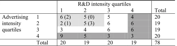
To check the robustness of the results, we also estimate the model so that the high and
low R&D industries are determined by quartiles of the R&D/sales-ratio. The high R&D
industries are in this case defined to be those in the highest quartile of the distribution. A
similar group is used for high advertising industries. We define as low sunk cost
median, i.e. in the two lowest quartiles. High sunk cost industries are such that either
R&D or advertising or both are in the top quartile. In these estimations the quartiles
where either R&D or advertising is in the third quartile and the other one in the bottom
three quartiles are left out. With this classification we have 36 high sunk cost industries,
18 low sunk cost industries, and 24 “middle” industries (see Table 2). Out of the sunk
cost industries, 19 have high R&D and 20 high advertising, so that only 3 industries have
both high R&D and high advertising intensity. The number of high R&D industries is
almost the same as in Table 1 where above average R&D intensity was used as the
cut-off point. This can be explained by the strongly skewed distribution of the R&D/output –
ratio. Among the 18 low sunk cost industries 6 have high import competition.
TABLE 2 HERE
How do other variables influence the level of concentration? They could be included into
the model in various ways. However, beyond the variables (setup costs and various
dummies and their interactions) that by theory should affect the bound, inclusion of other
variables directly as explanatory variables may not be justified. Instead, one could argue
that many of the other variables that potentially affect concentration should not influence
the lower bound, but rather determine how far different industries are from the bound.
While the bounds approach states that theory only gives the lower bound for
concentration, it is nevertheless interesting to see how deviations from the bound can be
explained by variables that have traditionally been used as determinants of concentration.
Our approach is to include this kind of variables in the mean µ and variance σ2u of the
truncated error component u.
We use the following variables in the mean and variance terms. Cost disadvantage ratio
(gross output per worker in plants producing less than the median plant, divided by the
corresponding figure for plants producing more than the median plant) takes into account
the costs that are caused by entry at suboptimal scale. Its impact on concentration should
be positive, since high cost disadvantage raises entry barriers. The variable also accounts
not measure the setup costs of those firms operating below the MES level (cf. Sutton,
1991, p. 95).
If the industry has many multi-plant firms, there may be economies in operating several
plants as opposed to operating in several single-plant firms. This may create a
disadvantage for entering firms that cannot start with several plants (Duetsch, 1984).
Multiplant economies are difficult to measure, so we use the variable share of multiplant
firms in the industry as a proxy measure of the importance of multiplant activity. It is
expected to have a positive impact on the deviation of actual concentration from the
lower bound.
We also include industry export intensity (share of production that goes to exports) as an
explanatory variable6. We argued above that it may be best not to include exports in the
equation that defines the lower bound. The impact of exports in the mean and variance of
u is not clear a priori either. On one hand, intense competition in export markets can have
effects similar to those of imports, i.e. higher concentration in the low R&D and low
advertising industries. On the other hand, it is possible that export markets make it
possible for more firms to survive in a country that has small domestic markets. This
would lead to lower domestic concentration.
4. Estimation results
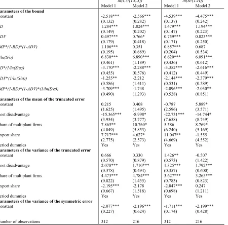
Table 3 presents the maximum likelihood estimation results for the model. Model 1 refers
to definition of R&D and advertising intensive industries based on the means of
R&D/sales and advertising/sales ratios, whereas Model 2 refers to definitions based on
the quartiles of the distributions of the ratios. The first two columns show the results
when C3 is the concentration measure and the last two columns for the Herfindahl index.
6 The export share data are from Industrial Statistics and available for all the years, in contrast to the
The estimated coefficient for high R&D dummy is positive and hence the hypothesis
about a higher lower bound for the R&D intensive industries gets support. The
comparison of import intensive and non-intensive industries with low sunk costs shows
that those industries that face tougher import competition have a higher lower bound, as
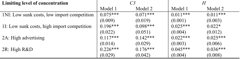
predicted. When S/σ approaches infinity, the constant term α in the model (Model 1) gives the limiting lower bound for ln(C3/(1-C3) in the low sunk cost, low import
competition industries. Hence, the limiting lower bound for C3 is eα/(1+eα). The limiting
bounds for the other industry groups are calculated in a similar manner. These limiting
concentration levels are shown in Table 4. Using the estimates of Model 1 in Table 3 the
implied limiting concentration ratio C3 is 0.226 for the high R&D intensity industries,
0.075 for the low sunk costs, low import competition industries and 0.196 for the low
sunk costs, high imports industries. As for advertising, the evidence is mixed. The
dummy for advertising intensive industries has a positive and significant coefficient, but
it is so low that the implied limiting concentration level is 0.117. This is above the
limiting concentration of the low sunk costs, low import competition industries, but
below that of the high import competition industries.
TABLES 3 AND 4 HERE
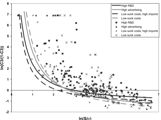
According to the theory, the bound should be less steep in the sunk cost industries. This
is, however, not quite supported by the results. The estimate for the slope coefficient is
highest (i.e., the slope steepest) for the reference group, low sunk costs, low import
competition industries. Advertising intensive industries have the second highest and
R&D intensive industries the third highest slope coefficient. The slope is the least steep
in the low sunk cost, high competition group. Figure 1 shows the deterministic parts of
the stochastic bounds.
FIGURE 1 HERE
We also report in Table 3 the coefficients of the variables in the mean and variance
on the effect of the variable on both µ and σ2u. Correspondingly, the total effect on Var(u)
depends on both terms (see Wang, 2002).7 These marginal effects, calculated for each
data point and averaged over the sample, are shown in Table 5. The share of multi-plant
firms has a highly significant positive effect both in the mean and variance equation. Also
the marginal effects on the mean and variance are positive. This is consistent with
multiplant economies. Since all the explanatory variables are shares, the magnitudes of
the marginal effects are such that, a one percentage point increase in a variable has a
marginal effect equal to an entry in Table 5 multiplied by 0.01. Hence, a one percentage
point increase in the share of multiplant firms would increase the mean E(u) by 0.05 and
the variance Var(u) by 0.22. Cost disadvantage has a negative sign in the mean equation,
but a positive one in the variance equation. The marginal impact on the mean is negative,
but but small, and the impact on the variance is positive (Table 5). Entry at suboptimal
scale may be costly, which contributes to high concentration in stretching the distribution
of deviations from the bound (although at the same time the distribution shifts slightly
closer to the bound). Finally, export share has a positive impact in the mean equation, but
a negative one in the variance equation. Its marginal impact on both the mean and
variance of the truncated error is negative. It seems that export activity makes it possible
for more firms to exist in a small market.
TABLE 5 HERE
To check the robustness of the results we defined the high and low sunk cost industries
on the basis of the quartiles of R&D and advertising intensity. The results on the
stochastic frontier are shown in column 2 of Table 3 and the limiting levels of
concentration in column 2 of Table 4. The constant for the low sunk costs, low import
competition group implies a limiting level of concentration 0.075 when market size
grows to infinity. The import competition dummy has non-significant coefficient. The
implied limiting level of concentration is 0.098. The limiting level of concentration for
7 In production models E(u) measures inefficiency and Var(u) can be interpreted as a measure of production
the high R&D intensity group is 0.176, and for the high advertising group 0.142. Except
for the high advertising group, these values are somewhat lower than in Model 1. The
results support the hypothesis that high sunk cost industries have higher limiting levels of
concentration. The slopes of the bounds for the high sunk cost industries are less steep
than for the other industries, as expected. As to the explanatory variables in the mean and
variance equations, the signs of the variables are the same as before, but the coefficient of
export share is not significant. The average marginal impacts on the mean and variance
are fairly similar to those in Model 1.
Finally, we carried out the estimations with the Herfindahl index as the measure of
concentration. The estimates using the two different definitions of R&D and advertising
intensity are shown in the last two columns of Table 3 and the limiting levels of the H
index in the last two columns of Table 4. The estimates agree with those obtained with
C3: The low sunk cost, low import competition industries have the lowest limiting H
-value and the steepest slope for the bound. The high R&D industries have the highest
limiting value for H and the least steep slope for the bound. The ranking of the low sunk
cost, high import competition and high advertising industries depends on the way the
high sunk cost industries have been defined. The main difference to the estimates with C3
in the impact of the other explanatory variables is that now cost disadvantage has a
negative marginal effect also on Var(u), although the magnitude of the effect is small.
With the alternative definition of sunk cost industries (Model 2), export share now has a
positive, but very small average marginal effect on Var(u).
All in all, the evidence gives mixed support for the endogenous sunk cost model. With
respect to R&D the results support the “bounds” approach, although the differences
between the limiting concentration ratios of high and low sunk cost industries are not big.
In case of advertising, the results are more inconclusive. One reason for this may be that
in an open economy sunk costs created by advertising by domestic firms is not that
important from the point of view of the market structure, if at the same time there is
advertising by foreign producers. Thus the main difference between industries seems to
industries the relevant markets are e.g. EU-wide (as in Lyons and Matraves, 1996), and in
small countries the theory does not fit well.
5. Conclusions
We have tested Sutton’s theory of concentration with Finnish data, using stochastic
frontiers to estimate lower bounds for concentration. It seems that in a small open
economy there are some features that need to be taken into account. First, in a small
country industries tend to be highly concentrated, which leads to difficulties in the use of
even 3-firm concentration ratios. We have adjusted the logit transformations of such
concentration ratios, although the adjustment is not unproblematic. The Herfindahl index
does not suffer from these problems and gives results that are consistent with those
obtained using the C3 concentration ratio. Another issue is how to treat foreign
competition. Rather than adjusting the concentration ratios for foreign trade, we have
treated import intensity as an indicator of competition. Consequently, we have allowed
for separate parameters for import intensive and non-intensive industries to test whether
the degree of competition affects the lower bound of concentration.
The results on R&D intensive and non-intensive industries seem consistent with the
predictions of the theory, although the differences between industries are not big. The
lower bound for the R&D intensive industries is at a higher level than that of low sunk
cost industries. On the other hand, among the low sunk cost industries, those facing tough
import competition have a higher limiting level of concentration than industries with less
foreign competition. As to advertising, the lower bound of concentration in advertising
intensive industries is at a lower level than in the industries with low sunk costs and high
import competition, which is in conflict with the theory. This result does, however,
change if we use another definition for the low sunk cost and high sunk cost industries. In
any case, it seems that in a small open economy the exposure to foreign competition is a
more decisive factor than advertising-related sunk costs. We have also tested whether
deviations of C3 from the lower bounds can be explained by observable industry
variance of deviations from the bound. This can be interpreted to be an effect of
multiplant economies. Export intensity had a negative impact on both. The results
indicate that export activity tends to allow more firms to exist, thereby lowering
concentration. Cost disadvantage of suboptimal scale plants had a positive effect on
variance, but a negative one on the mean of deviations from the lower bound. The impact
of scale-related entry barriers is therefore mixed.
References
Amemiya, T., Advanced Econometrics, Harvard University Press, 1985
Davies, S., ”Concentration”, in S. Davies et al., Economics of Industrial Organisation,
Longman, 1989, 73-126
Duetsch, L.L., “Entry and the extent of multiplant operations”, Journal of Industrial
Economics 32, 1984, 477-487
Giorgetti, M. L., Lower bound estimation – quantile regression and simplex method: An
application to Italian manufacturing sectors”, Journal of Industrial Economics 51, 2003,
113-120
Kumbhakar, S.C. and Lovell, C.A.K., Stochastic Frontier Analysis, Cambridge
University Press, 2000
Lyons, B. and Matraves, C., ”Industrial concentration”, in S. Davies, B. Lyons et al.,
Industrial Organization in the European Union: Structure, Strategy, and the Competitive
Mechanism, Oxford University Press, 1996, 86-104
Lyons, B., Matraves, C., and Moffatt, P., “Industrial concentration and market integration
in the European Union”, Economica 68, 2001, 1-26
Marin, P. L. and Siotis, G., “Innovation and market structure: An empirical evaluation of
the ‘bounds approach’ in the chemical industry”, CEPR Discussion Paper No. 3162, 2002
Robinson, W.T. and Chiang, J., ”Are Sutton’s predictions robust?: Empirical insights into
advertising, R&D, and concentration”, Journal of Industrial Economics 44, 1996,
Sutton, J., Sunk Costs and Market Structure – Price Competition, Advertising and the
Evolution of Concentration, MIT Press, 1991
Sutton, J., Technology and Market Structure – Theory and History, MIT Press, 1998
Sutton, J., “Market structure: The bounds approach”, in M. Armstrong and R. Porter,
eds., Handbook of Industrial Organization, vol. 3, Elsevier, 2006 (forthcoming)
Symeonidis, G., ”Price competition and market structure: The impact of cartel policy on
concentration in the UK”, Journal of Industrial Economics 48, 2000, 1-26
Wahlroos, B. and Backström, M., ”R&D intensity with endogenous concentration:
Evidence for Finland”, Empirical Economics 7, 1982, 13-22
Wang, H.-J., “Heteroscedasticity and non-monotonic efficiency effects of a stochastic
R & D intensity
Below average Above average Total Below average 37 (11) 15 52 Advertising
intensity Above average 21 5 26
Total 58 20 78
[image:21.595.83.418.126.183.2]Note: The industries in the shaded area are defined as high sunk cost industries and those in the unshaded area as low sunk cost industries. The number of high imports, low sunk cost industries is in parentheses.
Table 1. The number of industries in different groups, based on average values of R&D and advertising intensity (Model 1)
R&D intensity quartiles
1 2 3 4 Total 1 6 (2) 5 (0) 5 4 20 2 2 (1) 5 (3) 6 6 19 3 3 4 6 6 19 Advertising
intensity quartiles
4 9 5 3 3 20
Total 20 19 20 19 78
Note: The industries in the darker shaded area are defined as high sunk cost industries and those in the lighter shaded area as low sunk cost industries. The industries in the unshaded are were not used in the analysis. The number of high imports, low sunk cost industries is in parentheses.
[image:21.595.84.394.284.365.2]ln(C3/(1-C3)) ln(H/(1-H))
Model 1 Model 2 Model 1 Model 2
Parameters of the bound
Constant -2.518*** -2.566*** -4.539*** -4.475***
(0.132) (0.282) (0.137) (0.242)
RD 1.284*** 1.024*** 1.479*** 1.194***
(0.149) (0.202) (0.147) (0.223)
ADV 0.497*** 0.766* 0.759*** 0.823***
(0.179) (0.418) (0.171) (0.250)
IMP*(1-RD)*(1-ADV) 1.106*** 0.351 0.857*** 0.687
(0.195) (0.689) (0.204) (0.534)
1/ln(S/σ) 6.830*** 6.890*** 6.620*** 6.091***
(0.461) (1.189) (0.436) (0.612)
RD*(1/ln(S/σ)) -3.170*** -2.288*** -3.352*** -2.616***
(0.455) (0.576) (0.412) (0.449)
ADV*(1/ln(S/σ)) -1.255** -2.212 -2.144*** -2.379***
(0.586) (1.411) (0.531) (0.589)
IMP*(1-RD)*(1-ADV)*(1/ln(S/σ)) -3.709*** -1.748 -2.096*** -2.030**
(0.490) (1.293) (0.528) (0.851)
Parameters of the mean of the truncated error
Constant 0.215 0.408 -0.787 5.889*
(1.625) (1.495) (2.596) (3.571)
Cost disadvantage -15.365*** -8.998* -22.731*** -14.744*
(3.954) (3.777) (7.658) (8.749)
Share of multiplant firms 7.865** 10.760* 5.586 8.769*
(4.049) (5.853) (6.240) (5.169)
Export share 7.717*** 4.627* 11.047** -1.555
(2.775) (2.573) (4.669) (4.552)
Period dummies Yes Yes Yes Yes
Parameters of the variance of the truncated error
Constant 0.666 0.330 1.426** -0.507
(0.570) (0.879) (0.573) (1.422)
Cost disadvantage 2.078*** 1.710*** 1.325*** 1.792***
(0.378) (0.494) (0.357) (0.600)
Share of multiplant firms 4.473*** 4.784*** 3.627*** 3.265***
(0.822) (1.455) (0.783) (0.823)
Export share -2.195*** -2.178 -2.047*** 0.247
(0.667) (1.518) (0.698) (1.211)
Period dummies Yes Yes Yes Yes
Parameters of the variance of the symmetric error
Constant -2.077*** -2.196*** -1.711*** -2.199***
(0.227) (0.624) (0.174) (0.428)
Number of observations 312 216 312 216 Standard errors in parentheses. Significance level: *** 1%, ** 5%, * 10%.
[image:22.595.93.543.124.568.2]RD=dummy for high R&D intensity; ADV=dummy for high advertising intensity; IMP= dummy for high import competition.
Limiting level of concentration C3 H
Model 1 Model 2 Model 1 Model 2 1NI: Low sunk costs, low import competition 0.075*** 0.071*** 0.011*** 0.011***
(0.009) (0.019) (0.001) (0.003)
1I: Low sunk costs, high import competition 0.196*** 0.098*** 0.025*** 0.022*
(0.022) (0.051) (0.004) (0.012)
2A: High advertising 0.117*** 0.142*** 0.022*** 0.025***
(0.014) (0.029) (0.003) (0.006)
2R: High R&D 0.226*** 0.176*** 0.045*** 0.036***
(0.029) (0.042) (0.004) (0.008)
[image:23.595.84.502.147.250.2]Standard errors in parentheses. Significance level: *** 1%, ** 5%, * 10%.
Table 4: Limiting levels of concentration
ln(C3/(1-C3)), Model 1 ln(C3/(1-C3)), Model 2
E(u) Var(u) E(u) Var(u)
Average marginal effect of
Cost disadvantage -0.838 5.783 -1.042 2.632 Share of multiplant firms 5.053 22.619 6.378 18.784 Export share -0.541 -8.225 -0.440 -5.523
ln(H/(1-H)), Model 1 ln(H/(1-H)), Model 2
E(u) Var(u) E(u) Var(u)
Average marginal effect of
[image:23.595.81.432.321.462.2]Cost disadvantage -1.537 -0.692 -1.208 -0.041 Share of multiplant firms 3.031 7.071 3.829 7.443 Export share -0.195 -2.114 -0.086 0.094
-2 -1 0 1 2 3 4 5 6 7 8
0 1 2 3 4 5 6 7
ln(S/σ)
ln
(C3
/(
1
-C3
))
High R&D High advertising Low sunk costs, high imports Low sunk costs
[image:24.595.97.419.111.351.2]High R&D High advertising Low sunk costs, high imports Low sunk costs