Perishable Inventory Model Having Mixture of Weibull
Lifetime and Demand as Function of both Selling Price
and Time
Dr. R. John Mathew
*
Professor, Department of Computer Science and Engineering, Srinivasa Institute of Engineering and Technology, A.P, India
Abstract- In this paper we develop and analyse an inventory model for deteriorating items with mixture of Weibull rate of decay and demand as function of both selling price and time without shortages. Using the differential equations, the instantaneous state of inventory at time„t‟, the amount of deterioration etc. are derived. With suitable cost considerations the total cost function and profit rate function are also obtained by maximizing the profit rate function, the optimal ordering and pricing policies of the model are derived. The sensitivity of the model with respect to the parameters is discussed through numerical illustration. It is observed that the deteriorating parameters have a tremendous influence on the optimal selling price and ordering quantity.
Index Terms- Perishability, Instantaneous rate of deterioration, Total cost function, Profit rate function, the optimal ordering and pricing policies.
I. INTRODUCTION
uch work has been reported regarding inventory models for deteriorating items in recent years. In many of the inventory systems the major consideration is regarding the pattern of demand and supply. Goyal and Giri [4] have reviewed inventory models for deteriorating items. They also developed on the basis of demand variations and various other conditions or constraints. Various functional forms are considered for describing the demand pattern. Aggarwal and Goel [1] have developed an inventory model with the weibull rate of decay having selling price dependent demand. In reality, the demand rate of any product may vary with time or with price or with the instantaneous level of inventory displayed in a supermarket. Mathew [7] Roy and Chaudhuri [10], Sana [11], Tripathy and Mishra [13] have studied inventory models with demand rates depending on selling price of the item. Inventory problems involving time dependent demand patterns have received the attention of several researchers in recent years. Mathew [8] Chun, et al. [2], Giri, et al. [3], Manna, et al. [6], Mahata and Goswami [5] and Skouri, et al. [12] are among those who studied inventory models for deteriorating items having time dependent demand.
However, no serious attempt was made to develop inventory models for deteriorating items having mixture weibull rate of decay and both selling price and time dependent demand, which are very useful in many practical situations arising at oil and natural gas industry, photo chemical industries, chemical
processes, etc. Hence, in this paper we develop and analysed an inventory model with the assumption that the lifetime of the commodity is random and follows a three-parameter mixture weibull distribution having demand as a function of both selling price and time. Using differential equations the instantaneous state of on hand inventory is obtained. With suitable cost considerations the total cost function is derived. The optimal ordering policies are also obtained. The sensitivity of the model is analysed though numerical illustration. This model includes some of the earlier models as particular cases for specific or limiting values of the parameters.
II. ASSUMPTIONS AND NOTATIONS
We adopt the following assumptions and notations for the models to be discussed.
1.1 Assumptions
Assumption 1: The demand is known and is a function of unit selling price (s).
Assumption 2: Lead time zero Assumption 3: A deteriorating item is lost Assumption 4: The production rate is finite
Assumption 5: T is the fixed duration of a production cycle Assumption 6: The lifetime of the commodity is random and follows a three parameter
weibull distribution of the form f(t)= αβ(t-γ)β-1 eα(t-γ)β for t>γ
where α,β, γ are parameters.
Hence, the instantaneous rate of deterioration h (t) is h (t) =
αβ (t-γ) β-1 (2.1) 2.2 Notations
Q : The ordering quantity in one cycle of length T. A : The cost of placing an order.
C : The cost price of one unit.
H : The inventory holding cost per unit per unit time. S : The selling price of unit.
(s) : The demand rate, which is a function of unit selling price
III. INVENTORYMODEL
Consider an inventory system in which the amount of stock is zero at time t = 0. Replenishment starts at t = 0 and stops at t = t1 .The deterioration of the item start after a certain fixed lifetime
„‟. Since the perishability starts after „‟ the decrease in the inventory is due to demand during the period (0,), demand and deterioration during the period (, t1).During (t1, T) the inventory
level gradually decreases mainly to meet up demand and partly due to deterioration. By this process the stock reaches zero level at t = T. The cycle then repeats itself after time „T‟.
The schematic diagram representing the inventory system is shown in Fig.
Consider an inventory system in which the lifetime of the commodity is random and follows a mixture of three parameters weibull distribution with parameters1,1, 2,2, and p
Hence the instantaneous rate of deterioration h (t) as
H (t) =
1 2
1 1 2 2
2
1 2
1
1 ( t ) 1 ( t )
1 1 2 2
( t ) ( t )
p
(t
)
e
(1
p)
(t
)
e
pe
(1
p)e
for t > γ ; α1, α2,β1, β2, > 0 ; and 0 < p < 1 (3.1)
Along with all other assumptions made, assume that the demand rate is known and is a function of both selling price and time,
say
( , )
s t
. This functional form for the demand rate includes several functions involving selling price and / or time. To mention a few,(i) (s,t) =
(ii) (s,t) =
(iii) (s,t) = a
(iv) (s,t) = a
(v) (s,t) = , a constant, etc.
Where, s is the selling price per unit, T is the cycle length, r is the demand during the period T, n is the pattern index, a and b are known constants
Let „Q‟ be the ordering quantity in one cycle, „A‟ be the cost of placing an order, and „C‟ be the cost of one unit, „h‟ be the inventory holding cost per unit per unit time. (s,t) is assumed such that the total cost function is convex. In this model the stock decreases due to (i) the demand of items in the interval
(0,), (ii) the combination of deteriorating and demand of items in the interval (,t),(iii) during (t1,T) the inventory level gradually
decreases mainly to meet up demands and partly for deterioration, by this process the stock reaches zero level at t=T. The cycle then repeats itself after time T.
Let I (t) be the inventory level of the system at time t (0 < t <T). Then, the differential equations describing the instantaneous states of I (t) over the cycle of length T are
1 1
1 ( )
n
n
d srt
I t k dt
nT
for 0 < t < γ (3.2)
1 1
1
( ) ( ). ( )
n
n
d srt
I t h t I t k dt
nT
for γ < t < t1 (3.3)
1 1
1
( ) ( ). ( )
n
n
d srt
I t h t I t dt
nT
I (t) =
1 1
1
n
n
srt
k
nT
0 < t < γ (3.5)
I (t) =
1 2
1 2
1
p
(
t
)
(1
p
)
(
t
)
1
1 2
1 1
1 1
1 2 1 1
1 ( ) (1 ) ( ) ,
t n n
n n
sru sr
p u p u k du kr
nT T
γ < t < t1 (3.6)
I (t) =
1 2
1 2
1
p
(
t
)
(1
p
)
(
t
)
1 2 1 2
1 1
1 1
1 1
1 2 1 2
1
(
)
(1
)
(
)
1
(
)
(1
)
(
)
,
T t
n n
t t
t
p
t
p
t
dt
u
p
t
p
t
du
(3.7)The stock loss due to deterioration in the interval (0, T) is
L (T) =
1 1
1 1
n n srt kt
nT
(3.8)
The ordering quantity in a cycle of length T is obtained as
Q = kt1 (3.9)
Let K (t1, T, s) be the expected total cost per unit time. Since the total cost is the sum of the set up cost, cost of the units, the
inventory holding cost. K (t1, T, s) is obtained as
K (t1, T, s) =
1
1 0
( )
( )
( )
t T
t
A
cQ
h
h t dt
h t dt
h t dt
T
T
T
(3.10)using Taylor‟s series expansion for the exponential function for small values of α(t – )β , the power series expansion and ignoring the higher order terms we get,
1
22
2 2
1 1 1 2
1 1 1
1 2 2 2
2
( , , )
2(1
)
2
1
2
1
2
kct
t
p
A
hk
K t T s
t
p
t
T
T
T
1 1
1 2
1 2
1 1 1
1 2
(
)
(1
)
(
)
1
1
p
t
p
t
t
1 1
1 1 1 1
1 1
1
1 1 1 1
1
1 1 1
1 1
1 1
1 1
1 1
1 1
1 1 1 1
n n
n n n n
n
p hsr
t t
n n n
T
n n
2 2
2 2 2
2
1 1
1
1 1 1 1
1 1
2 2 2
1 1
2 2
2 2
(1 ) (1 )
1 1
1 1 1
n n
n n n n
p t p t
n n n
n n
1 2
1 2
1 1 1
1 1 1
1 n 1 n 1 n 1
1 1 1
1 n 1 1 2 n 2 2 n n
1 1
1 n
1 1 2 2
p hsr T
p (1 p) (1 p) T t T
1 1 1 1 1
1 1 T 1
n n n n n
1 1 1
1 1 1 1 1 1
1
1 1 1
1 1
1 1 1 n 1 n 1 1 1 1 n 1
1 n n 1 1 n n 2 n n
1 1 1
1 2
1 1 2
p T p T (1 p) T
T t T T T t T T t
1 1 1
n 1 n n 1 n 1
1 1
n n n
1 1 2 2 2 1 1 1 1 1 1
1 n 1 1 1 1 n n
1 1
2 2 n n 2 n n 1 1 1
1 1
2 1
2 1 1
p T T
T
(1 p) T T t T (T ) T (t ) p p
1 1 1
n n 1 1 1
n n n
2 2 1 2
1 1 1 1
1
1 1
2 n n 2 n 2 2 n
1 2 2
2
2 2
(1 p) T (T ) T (t ) (1 p) .t (1 p) t
1 1 1 1 n n
(3.11)
Profit rate function P (t1,T,s) is P (t1,T,s) = sλ(s) - K ((t1,T,s)
1
1 11 2 1 0
. .
( , ,
.
, T,
)
T n
n
s
s r t
dt
K t t s
T
n
t
s
T
P
= 2 2 1 2 2 21 1 1 2
1 1
1 1 2 2
2
(
)
2(1
)
(
)
2
(
1)(
2)
(
1)(
2)
ckt
t
p
s r
A
hk
t
p
t
T
T
T
T
11 2 1 1 1
1
1 1
1 1
1 2 1
1 1 1 1 1 1
1
1 2 1
1
( ) (1 ) ( )
1
1 1 1 1
n
n n
n
hsr
p t t p t t p t
n T n 1 2
1 1 2 2
1 1
1
1 1 1 1
1 1
1 1 2
1 1
1 2
1 2
(1 )
1 1
1 1 1 1
n n
n n n n
p
t p t
n n n
n n 1 2
1 2 2
1 1
1
1 1 1
1 1
1 1 1 2 2
1 2
1 1 2
(1 )
1 1 1 1 1
n n
n p n n
p p t
n n
n n n
2 1
2 1 1
1 1 1
1 1 1
1 n 1 n 1 1 1 n
1 1 1
2 n 2 2 n n 1 n n
1 1
1 1
1 n
2 2 1
p
hsr T T
(1 p) (1 p) T t T T t T
1 1 1 1 1 n 1 1 1
T
n n n n
1 1
1 1 1 1
1
1 1
1
1 n 1 1 1 1 n 1
1 1 n n 2 n n
1 1
2
1 2
p T (1 p) T
T T t T T t
1 1
n n 1 n 1 1
n n 2 2 2 1 1 1
1 n 1 1 1
1
1 1
2 2 n n 2 n n
1 1
2 1
2
p T
(1 p) T T t T (T ) T (t )
1
n n 1 1
1 1
2 2
1 2
1 1
1 1 1 1 1
n n 1
1 1
1 1 1 2 n n 2 n 2 2 n
1 2
1 1 2 2
T T
p p (1 p) T (T ) T (t ) (1 p) T (1 p) T
1 1 1 1 1 1 1
n n n n
IV. OPTIMALPOLICIESOFTHEMODEL
In this section the optimal pricing and ordering policies of the inventory system by taking a specific form the demand is discussed. Let the demand rate be of the form
1 1
1
( , )
n
n
srt
s t
nT
(4.1)
which indicates that the demand as an increasing function of time and selling price. This situation prevails in oil exploration industry.
To find the optimal values of t1, T, s equate the first order partial derivatives of P (t1, T, s) with respect to t1, T and s to zero.By
differentiating P (t1, T, s) given in equation (3.12) with respect to t1 and equating to zero, we get
1 1
2 2
1
21 2
1 1 1 1 1 1 2 2 1
1 2
(1
)
(1
)
1
1
kc
hk
t
p
t
p
t
pt
t
p t
t
T
T
2 1 2 2
1 1 1 1
1 1 1 2 2 2
1 1
1 2 2 2
(1 ) (1 )
1 1 1 1
n n n n
n hsr
p p p p
n n n n n n
T
2 1 2 2
1 1 1 1 1
1 1
1 1 1 2 2 2
n n n n n
1 1
1 2 2 2
n
hsr
T
p
T
p
T
(1 p)
T
(1 p )
T
n
1
n
n 1
n
1
n
n 1
T
1
21 1
1 1
(1
)
2 10
N N
p T
t
p
T
t
(4.2)By differentiating P (t1, T, s) with reference to T and equating to zero, one can get
1 2
2
2 2
2 1 1 2
1 1 1
1 2 2 2
t
2p
hk
s r
A
kct
(t
)
2(1 p)
(t
)
T
2
(
1)(
1)
(
1)(
2)
1 1 2 1
1 2
1 1 1 1
1 2
p
(t
)
t
(1 p)
(t
)
t
1
1
1 1
1 1 1 1
1 1
1
1 1 n 1 1 n 1 1
1 n n 1 1 n n
1 1
1
1 1
n
1 1
hsr
p t p t
1 1
n 1 1 n n 1 1
T
n n
2 2
2 2 2 2
1 1
1
1 1 n 1 1 n 1 1
2 n n 2 2 n n
1 1
2 2
1 2
(1 p) t (1 p) t
1 1
n 1 n n 1
1
n n
1 1 2 2
1 1 1 1
1 1 1 1
1 1 1 2 2 2
1 1 2 2
(1 ) (1 )
1 1 1 1
1 1
n n n n
p p p p
n n n n
1 1
1 1 1 1
1 2
1 2 2 2
2 1 1 1 1 1 1
1 1 1 1 1 1
2
1 1
1 1
( 1)
( 1) ( 1) ( 1)
1 1
1 1 1
t p T p T
hsrT T t T T t T
T n n n
n n 2 2
2 1 2 1
2 2
2 2 2
2 2 2 2 2
1 1 2 2 1
2
2 2
(1 ) ( 2) (1 ) ( 1)
( 1) ( 1) ( 2)
1 1
1 1
1
p T p T
T T t T T t
nT n n
n n
1 2 2 1
1 1
1 1 1 1 1 1
2 1 1 1 1 1 1 2 2
2 2
1
1 2 2
( 1)( ) ( ) ( ) ( 1)
(1 )
1 1 1
1 1 1
p T T r T r T r p T p T p T
p
T T
n n n
2 2
2 2 1 2 1
2 2 1 2 2
2 2
2
2
( 1)( ) ( ) ( ) (1 ) ( 1)
(1 ) 0
1 1
T T r T r t r p T T
p T T n
(4.3)
Differentiating P (t1, T, s) with reference to s and equating to zero, we get
1 1
1 1 1 1
1 1
1
1 n 1 1 n 1
1 1
1 n n 1 1 n n
1 1 1 1 1 1 n 1 1 p 2rs hr
p t t
1 1
T n 1 1 n n 1 1
T n n 1 2
2 2 2 2
1 1
1
1 1 n 1 1 n 1 1
2 n n 2 2 n n
1 1
2 2
2 2
(1 p) t (1 p) t
1 1
n 1 1 n n 1
n n 1 2 1 2
1 1 1
1 1 1
1 1 n 1 1 n 1 1 n 1
1 n 1 1 2 n 2 2 n n
1 1
1 n
1 1 2 2
p hr T
p (1 p) (1 p) T t T
1 1 1 1 1
1 1 T 1
n n n n n
1 1 2
1 1 1 1 2 1
1 1 1
1 1
1 1 1 n 1 n 1 1 1 1 n 1
1 n n 1 1 n n 2 n n
1 1 1
1 1 2
1 1 2
p T p T (1 p) T
T t T T T t T T t
1 1 1
n 1 1 n n 1 n 1 1
n n n
2 2 2 1 1 1
1 n 1 1 1
1 1 1
2 2 n n 2 n n
1 1
2 1
2
p T
(1 p) T T t T (T ) T (t )
1
n n 1 1
n 1 1 2 2 1 2 1 1
1 1 1 1 1
n n 1 1 1
1 1 1 2 n n 2 n 2 2 n
1 2
1 1 2 2
T T
p p (1 p) T (T ) T (t ) (1 p) T (1 p) T 0
1 1 1 1 1 1 1
n n n n
(4.4)
Solving the equations (4.2), (4.3) an (4.4) numerically for given values of T, 1,1, 2,2,,p, r ,n, A, c, and h one can
obtain the optimal values of t1* of t1, T* of T, and s * of s. also
obtain the optimal expected total cost per unit time. Even though T is fixed the expected total cost is function of T. So the expected cost function is effected by the various values of T. Hence the optimal cycle length can also be obtained by using search methods after substituting the optimal value of t1*, t2*,s* and Q*
as initial values.
V. NUMERICALILLUSTRATION
For various values of 1,1, 2,2,,p and T the optimal
values of t1*,t2*,s* and Q* are computed by solving the
production process is maximum then the selling price and the ordering quantity are optimal.
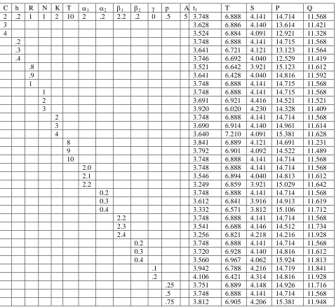
Table – 1
Optimum values of production time, selling price, profit and ordering quantity
C h R N K T 1 2 1 2 p A t1 T S P Q
2 .2 1 1 2 10 2 .2 2.2 .2 0 .5 5 3.748 6.888 4.141 14.714 11.568
3 3.628 6.886 4.140 13.614 11.421
4 3.524 6.884 4.091 12.921 11.328
.2 3.748 6.888 4.141 14.715 11.568
.3 3.641 6.721 4.121 13.123 11.564
.4 3.746 6.692 4.040 12.529 11.419
.8 3.521 6.642 3.921 15.123 11.612
.9 3.641 6.428 4.040 14.816 11.592
1 3.748 6.888 4.141 14.715 11.568
1 3.748 6.888 4.141 14.715 11.568
2 3.691 6.921 4.416 14.521 11.521
3 3.920 6.020 4.230 14.328 11.409
2 3.748 6.888 4.141 14.714 11.568
3 3.690 6.914 4.140 14.961 11.614
4 3.640 7.210 4.091 15.381 11.628
8 3.841 6.889 4.121 14.691 11.231
9 3.792 6.901 4.092 14.522 11.489
10 3.748 6.888 4.141 14.714 11.568
2.0 3.748 6.888 4.141 14.714 11.568
2.1 3.546 6.894 4.040 14.813 11.612
2.2 3.249 6.859 3.921 15.029 11.642
0.2 3.748 6.888 4.141 14.714 11.568
0.3 3.612 6.841 3.916 14.913 11.619
0.4 3.332 6.571 3.812 15.106 11.712
2.2 3.748 6.888 4.141 14.714 11.568
2.3 3.541 6.688 4.146 14.512 11.734
2.4 3.256 6.821 4.218 14.216 11.928
0.2 3.748 6.888 4.141 14.714 11.568
0.3 3.720 6.928 4.140 14.816 11.612
0.4 3.560 6.967 4.062 15.924 11.813
.1 3.942 6.788 4.216 14.719 11.841
.2 4.106 6.421 4.314 14.816 11.928
.25 3.751 6.889 4.148 14.926 11.716
.5 3.748 6.888 4.141 14.714 11.568
.75 3.812 6.905 4.206 15.381 11.948
From Table 1 it is observed that the optimal ordering quantity, and the expected total cost per unit time are much influenced by the parameters, various costs and cycle length. It is observed that as cycle length increases, the optimal ordering quantity is increasing when the other parameters and cost are fixed. The optimal ordering quantity is also influenced by the mean lifetime of the commodity. The optimal ordering quantity is very sensitive to the penalty cost, when other parameters are fixed. When the penalty cost is increasing, the optimal ordering quantity is increasing. However if the increase in the penalty cost is in proportion to the increase in the cost per unit, then the optimal ordering quantity is an increasing function to the increase in the cost. If the cost per unit is much higher than the penalty cost, then the optimal ordering quantity is a decreasing
two parameters on the optimal values of their inventory models with respect to their inter-relationship Even though T, the cycle length is considered to be a known value in this inventory model, it is also interesting to note that the cycle length has a vital influence on the optimal ordering quantity and expected total cost per unit time. For deriving the optimal ordering quantity one has to properly estimate the parameters involved in the lifetime of the commodity.
VI. CONCLUSIONS
Inventory models play a dominant role in manufacturing and production industries like cement, food processing, petrochemical, and pharmaceutical and paint manufacturing units. In this paper, an inventory model for deteriorating items with constant rate of replenishment, time and selling price dependent demand and mixed Weibull decay has been developed and analyzed in the light of various parameters and costs and with the objective of maximizing the total system profit. The model was illustrated with numerical examples and sensitivity analysis of the model with respect to costs and parameters was also carried out. This model also includes the exponential decay model as a particular case for specific values of the parameters. The proposed model can further be enriched by incorporating salvage of deteriorated units, inflation, quantity discount, and trade credits etc. It can also be extended to a multi-commodity model with constraints on budget, shelf space, etc., These models may also be formulated in fuzzy environments.
REFERENCES
[1] Aggarwal, S.P., Goel, V.P (1984) Order Level inventory system with demand pattern for deteriorating items, Econ. Comp. Econ. Cybernet, Stud. Res.,Vol. 3,57- 69.
[2] Chun Chen Lee, Su-Lu Hsu, (2009) “A two-warehouse production model for deteriorating items with time-dependent demands”. European Journal of Operational Research, Vol.194, Issue 3, 700-710.
[3] Giri, B.C., Goswami, A. and Chaudhuri, K. S. (1996). An EOQ model for deteriorating items with time varying demand and costs. Journal of the Operational Research Society, Vol.47, 1398-1405.
[4] Goyal, S.K., Giri, B.C (2001) Inview recent trends in modeling of deteriorating inventory, EJOR, Vol. 134, 1-16.
[5] Mahata G. C. and Goswami A. (2009a) „Fuzzy EOQ Models for Deteriorating Items with Stock Dependent Demand & Non-Linear Holding Costs‟, International Journal of Applied Mathematics and Computer Sciences 5;2, 94-98.
[6] Manna, S.K., Chaudhuri, K.S. and Chiang, C. (2007) „Replenishment policy for EOQ models with time-dependent quadratic demand and shortages’,
International journal of Operational Research, Vol. 2, No.3 pp. 321 – 337. [7] Mathew, R.J., Narayana, J.L. (2007) Perishable inventory model with finite
rate of replenishment having weibull lifetime and price dependent demand Assam Statistical review (2007), Vol. 21, 91-102. [8] Mathew, R.J(2013) Perishable inventory model with finite rate of
replenishment having weibull lifetime and time dependent demand .Accepted by International journal of mathematical archive,IJMR;4 - 228 [9] Ritchie, E. (1984). The EOQ for linear increasing demand, A simple
optimum solution. Journal of the Operational Research Society, Vol.35, 949-952.
[10] Roy T. and Chaudhuri K.S. (2010) „Optimal pricing for a perishable item under time-price dependent demand and time-value of money‟,
International Journal of Operational Research, Vol. 7, No.2, 133 – 151. [11] Sana S.S. (2011) „Price-sensitive demand for perishable items – an EOQ
model‟, Applied Mathematics and Computation, Vol. 217, 6248–6259. [12] Skouri, K., Konstantaras, I., Papachristos, S., Ganas, I., (2009) „Inventory
models with ramp type demand rate, partial backlogging and Weibull deterioration rate‟, European Journal of Operational Research, Vol. 192 (1), 79–92.
[13] Tripathy C.K., Mishra.U, (2010) “An inventory model for weibull deteriorating items with price dependent demand and time-varying holding cost”. Applied Mathematical Sciences, Vol. 4, No.44, 2010, 2171-2179
AUTHORS
First Author – Dr. R. John Mathew, Professor, Department of