http://ijmms.hindawi.com © Hindawi Publishing Corp.
A HIGHER-ORDER METHOD FOR NONLINEAR SINGULAR
TWO-POINT BOUNDARY VALUE PROBLEMS
K. M. FURATI and M. A. EL-GEBEILY
Received 18 May 2001 and in revised form 3 October 2001
We present a finite difference method for a general class of nonlinear singular two-point boundary value problems. The order of convergence of the method for such a general class of problems is higher than the previous reported methods. The method yields a fourth-order convergence for the special casep(x)=w(x)=xα,α≥1.
2000 Mathematics Subject Classification: 65L10.
1. Introduction. We consider the class of nonlinear singular two-point boundary value problems
−w(x)1 p(x)y(x)=g(x, y), x∈(0,1),
py0+=0, y(1)=0,
(1.1)
under the following assumptions:
(A1) for(x, y)∈[0,1]×R, the functiong(x, y)is continuous with continuous non-positive derivativegy=∂g/∂y;
(A2) g(x) = g(x, y(x)) ∈ Cm+1[0,1], for some integer m ≥ 0, whenever y ∈ Cm+1[0,1];
(A3) p−1(x)=1/p(x)is nonnegative and integrable on any compact subset of the interval(0,1];
(A4) w(x)is nonnegative and integrable on[0,1]; (A5) 01(
1
t p−1(τ)dτ)w(t)dt <∞.
Under these assumptions, it was shown in [8] that the boundary conditions assumed here are possible and problem (1.1) has a unique solutiony(x)which is absolutely continuous on[0,1].
Singular boundary value problems occur in many applications such as transport pro-cesses, thermal explosions, and electrohydrodynamics. (References are given in [4].)
Standard numerical methods exhibit loss of accuracy or even lack of convergence when applied to singular problems. (For more details please see [5,9].)
For the linear problem, Abu-Zaid and El-Gebeily [1] generalized the method in [3] tow(x)=p(x). Recently, El-Gebeily and Abu-Zaid [7] relaxed this requirement and several other assumptions, however, the order of convergence of their scheme is at most 2.
We construct a higher-order method for the nonlinear problem (1.1). Unlike the previous treatment, this method is designed to work for generalpandwwhich are not even required to be smooth. The higher order of convergence is obtained by ap-proximating the functiongby a quadratic interpolating polynomial. This method is fourth order for the casep(x)=w(x)=xα,α≥1, and at least third order for the class of problems considered in [1]. Quadrature methods can also be used to set up the integrals associated with this method. So, knowledge of the exact integrals is not necessary (except for those integrals that involve singularities).
We start by constructing the finite difference method. Then we analyze the error and find the rate of convergence. Finally, we present some numerical examples.
2. Exact discretization of the problem. In this section, we present the exact dis-cretization of (1.1). We first introduce special sets of basis functions that we use for the discretization. Then we get a system of equations for the exact solution at the mesh points. Our working space is the space of continuous functions on the interval[0,1]. Letπ= {0=x0< x1<···< xN=1}be a given partition of the interval[0,1]. We associate two sets of basis functions with the nodesx1, x2, . . . , xN−1of this partition:
(1) the setU1, U2, . . . , UN−1given by
U1(x)=
1, x0≤x≤x1, ψ1(x)
ψ1x1, x1≤x≤x2, 0, otherwise,
(2.1)
and for 2≤k≤N−1
Uk(x)=
1− ψk−1(x)
ψk−1xk−1, xk−1≤x≤xk, ψk(x)
ψkxk, xk≤x≤xk+1,
0, otherwise,
(2.2)
whereψk(x)=xk+1
x p−1(t)dt;
(2) the local basis setik,i=k−1, k, k+1,k=1,2, . . . , N−1, of piecewise quadratic interpolating polynomials defined on each subintervalIk=[xk−1, xk+1]by
ik(x)= k+1 j=k−1, j≠i
x−xj
xj−xi, (2.3)
and zero outsideIk. We assume that
This assumption is satisfied by many standard problems. For example, one can show, by direct calculations, that this is the case whenw(x)=p(x)=xα.
Letᏼkbe the projection
ᏼk:C[0,1] →CIk,
ᏼkf (x)= 1
j=−1
fk+jk+j,k(x), (2.5)
wherefi=f (xi),i=0,1, . . . , N−1. Iff∈C3(Ik), then
I−ᏼkf=
fξk 3!
k+1
i=k−1
x−xi, (2.6)
for someξk∈Ik.
By multiplying both sides of (1.1) byUk,k=1, . . . , N−1, and integrating over the interval[0,1], we get
−py, Uk= g, wUk
, (2.7)
where·,·is defined by
α1, α2= 1
0
α1(x)α2(x)dx. (2.8)
Note thatUkis absolutely continuous on[0,1]fork=1, . . . , N−1. Therefore, if a func-tiony∈C[0,1]is such that(py)is integrable, then−(py), Uk =py, Uk . Ify is a solution of the boundary value problem (1.1), then our assumptions on the func-tionsp,g,w imply that(py)is integrable. Hence, integration by parts is justified in our case.
It can be easily checked that the integrals in the left-hand side of system (2.7) take the more explicit form
− py, U1= −ψ11 x1y2+
1 ψ1x1y1, − py, Uk= py, Uk= y, pUk
= −ψk1
xkyk+1+
1
ψk−1xk−1+ 1 ψkxk
yk−ψk 1 −1xk−1
yk−1, (2.9)
fork=2, . . . , N−1, where yi=y(xi). Also, by introducing the projectionsᏼk into system (2.7), we get
py, Uk= ᏼkg, wUk+ I−ᏼk
g, wUk, (2.10)
with
ᏼkg, wUk= k+1 i=k−1
wheregi=g(xi, yi). Note thatgN=g(1,0)whileg0=g(0, y0)involves the unknown value of the solution atx=0. We will deal with this difficulty later. It is known (see [8]), however, thaty0exists and is finite under our assumptions.
In matrix form, system (2.7) can be written as
T Y=LG(Y )+B(Y )+Q+R, (2.12)
where
Y=y1, . . . , yN−1t, G(Y )=g1, . . . , gN−1t,
T=tridiagtk, δk, tk+1,
L=tridiagl(k)k−1, l(k)k , l(k)k+1,
B(Y )=l(1)0 g0,0, . . . ,0t,
Q=0, . . . ,0, l(N−1)N gN t
,
R= I−ᏼ1g,wU1, . . . , I−ᏼN−1g,wUN−1t,
(2.13)
with
tk+1= − 1
ψkxk, k=1, . . . , (N−2),
δ1= −t2, δk= −tk+1+tk, k=2, . . . , (N−1),
l(k)i = ik, wUk
, i=k−1, k, k+1, k=1, . . . , N−1.
(2.14)
For x ∈[0, x1], following the same derivation in [7], we can show the following identity:
y(x)=y1+ x
0 x1
x p
−1(τ)dτw(t)g(t)dt
+ x1
x x1
t p
−1(τ)dτw(t)g(t)dt.
(2.15)
In particular, at the singular pointx=0, identity (2.15) reduces to
y0=y(0)=y1+ x1
0 x1
t
p−1(τ)dτ
w(t)g(t)dt, (2.16)
which can also be written as
y0−y1= g, wU0+
, (2.17)
where
U0+(x)=
x1
x p
−1(t)dt, 0< x≤x1,
0, otherwise.
By expandingg(x)about(x, y1), we get forx∈(0, x1),
g(x)=gx, y(x)=gx, y1+gyx, y(ξ)y−y1, (2.19)
for someξ∈(x, x1). Now, by using (2.17) and (2.19), we get the identity
y0=y1+ g·, y1, wU0+
+ gy·, yξ(·)y−y1, wU0+
. (2.20)
3. Numerical method and error analysis. The setup carried out inSection 2 indi-cates that we intend to obtain a numerical method by truncating the remainder term Rin (2.12). However, one difficulty remains which is, how to obtain the value ofg0. To overcome this difficulty we notice that the basis functionU1(x)is always unity on the interval[0, x1]. This means that we may use an approximate value ofy1, ¯y1, as an approximate value fory0, and thus approximateg0=g(0, y0)by ¯g0=g(0,y1)¯ . The fact that this approximation does not affect the overall order of the method remains to be shown.
Using this approximation ofg0and truncating the remainder termRin (2.12), we obtain a numerical method that determines an approximation ¯Y =[y1, . . . ,¯ yN¯ −1]t of Y from
TY¯=LG(Y )¯ +B(Y )¯ +Q. (3.1)
Then, the approximate value ¯y0ofy0is calculated using
¯
y0=y1+¯ g·,y1¯ , wU0+. (3.2) For the error analysis, letE=Y−Y¯=[e1, e2, . . . , eN−1]t. Then, from (2.12) and (3.1), we get
T E=LG(Y )−G(Y )¯ +B(Y )−B(Y )¯ +R. (3.3)
Using the integral form of the mean value theorem, we write
G(Y )−G(Y )¯ = 1
0G
tY+(1−t)Y¯(Y−Y )dt¯ =DE, (3.4)
whereG(Z)=diag(gy(xi, zi))forZ=[z1, . . . , zN−1]t, andD=diag(di), where
di= 1
0gy
xi, tyi+(1−t)yi¯dt. (3.5)
For the termB(Y ), we write an error representation as follows: letJ=[1,0, . . . ,0]t, then
B(Y )−B(Y )¯ =l(1)0
g0−g0¯ J=l(1)0 J 1
0gy
0, ty0+(1−t)y1¯ y0−y1¯ dt
=l(1)0 d0y0−y1¯ J=l(1)0 d0 1J+l(1)0 d0e1J =l(1)0 d0 1J+F E,
where 1=y0−y1,F=diag(J)l(1)0 d0, and
d0= 1
0gy
0, ty0+(1−t)y1¯ dt. (3.7)
Hence, the error equation (3.3) can be rewritten as
(T−LD−F )E=l(1)0 d0 1J+R. (3.8)
Note that the entries ofDas well asd0are nonpositive sincegy≤0. The matrixT has the following properties:
(1) T is tridiagonal and diagonally dominant, (2) the diagonal elements are positive, (3) tktk+1>0, fork=1, . . . , (N−2).
It follows from these properties thatT is irreducible and thusT is irreducibly diago-nally dominant (see [10, pages 47–55]). Moreover, since the off-diagonal elements are nonpositive,T is anM-matrix.
From (2.4), we haveL≥0. This implies thatLD≤0 andF≤0. Therefore,T−LD− F≥ T. Also,T−LD−F is anM-matrix. To see this, notice that
l(k)k+1 tk+1 =
ik, wUk 1/ψkxk ≤
xk+1
xk−1 w(x)
xk+1
x
p−1(t)dt
dx, (3.9)
fork=1,2, . . . , N−1, since|ik| ≤1. It follows that forh=max0≤k≤N−1{xk+1−xk} sufficiently small, the off-diagonal elements of T dominate the corresponding ele-ments ofLD. Hence, for sufficiently small h, T−LD−F is an M-matrix and thus (T−LD−F )−1≤T−1(see [10]). Therefore, we have
E ∞≤T−1l(1)0 d0 1J+R∞, (3.10)
where the matrixT−1=(τkj)is given by
τkj=
1 xj
p−1(x)dx, k≤j, 1
xk
p−1(x)dx, k≥j.
(3.11)
It follows from (2.6) that for 1≤k≤N−1, (I−ᏼk)g ∞≤ch3 g ∞, and thus
I−ᏼk
g, wUk≤I−ᏼk
g∞ 1, wUk≤ch3g
∞ 1, wUk
. (3.12)
Since the first row ofT−1includes the largest element in each column, it follows fromLemma A.2that
T−1|R|∞≤c N−1
k=1
I−ᏼk
g, wUk 1
xk
p−1(t)dt
≤ch3g∞ N−1 k=1
1, wUk 1 xk
p−1(t)dt
=ch3g∞ N−1 k=1
xk+1
xk−1w(t)Uk(t)dt 1
xkp
−1(t)dt
≤2ch3g ∞
N−1
k=1 xk+1
xk−1 1
t
p−1(τ)dτ
w(t)dt
≤4ch3g∞ 1
0 1
t p
−1(τ)dτw(t)dt
(3.13)
for some constantc >0. For the other term in the error equation (3.8), we have, from (2.20),
1=y0−y1 = g·, y1, wU0+
+ gy·, yξ(·)y−y1, wU0+ ≤ g ∞ 1, wU0++gy∞ y−y1, wU0+,
(3.14)
and from (2.15) andLemma A.1,
y−y1≤ g ∞ 1, wU0+. (3.15)
Thus,
1≤ g ∞ 1, wU0++ g ∞gy∞ 1, wU0+2=O 1, wU0+. (3.16)
Also from (3.7),d0≤gy∞. Hence, T−1l(1)0 d0 1J∞=l(1)0 τ11d0 1
=Ol(1)0 τ11 1, wU0+
=O 1, wU0+ x2
0 w(t) 1
t p
−1(τ)dτdt
=O
1, wU0+2+ x2
0 w(t)
1 t
p−1(τ)dτ
dt 2
=O x2
0 w(t)
1 t
p−1(τ)dτ
dt 2
.
(3.17)
It follows from (3.13) and (3.17) that the order of the error in scheme (3.1) is
E ∞=Oh3+O
2h
0 w(t) 1
t p
−1(τ)dτdt2
. (3.18)
As for the error in computingy0, we have from (2.20), (3.2), and (3.15) y0−y0¯ =y1−y1¯ + g·, y1−g·,y1¯ , wU0+
+ gy·, yξ(·)y−y1, wU0+ ≤y1−y1¯ +gy∞y1−y1¯ 1, wU0++gy∞ g ∞ 1, wU0+2
=O E ∞+O 1, wU0+2
=O E ∞+O
2h
0 w(t)
1 t
p−1(τ)dτ
dt 2
.
(3.19)
Thus we have proved the following theorem.
Theorem3.1. Under the assumptions (A1), (A2), (A3), (A4), (A5), and (2.4), the finite difference scheme (3.1) and (3.2) converges uniformly to the solution of (1.1) with order of convergence of at least
Oh3+O
2h
0 w(t)
1 t
p−1(τ)dτ
dt 2
. (3.20)
Remark 3.2. If the error term 1, wU0+2 is of less order than the error term |y−y1|¯ , then more accuracy may be achieved by taking more terms in the expan-sion ofgabouty1. In principle, we get an error term of order1, wU0+m+1, wherem is the number of derivatives taken in the Taylor series expansion ofg.
Remark3.3. In the approximation (3.2), the exact integralg(·,y1), wU¯ 0+is com-puted. If this integral cannot be found in closed form or if it is too complicated, then it has to be computed numerically. This can be done by replacingg(·,y1), wU¯ 0+by
gx1,y1¯ 1, wU0++∂g ∂x
x1,y1¯ ·−x1, wU0+. (3.21) This results in the extra error term
∂2 ∂x2g
η(·),y1¯ ·−x12, wU0+
, (3.22)
which is of orderh21, wU+ 0.
Remark3.4. For the special casep(x)=w(x)=xα,α >1, or if the differential equation is regular, the summation term in (3.13) is of orderh4. Also, the second term of (3.20) is of orderh4. So the method is fourth-order accurate as should be expected since our method and the method given in [4] are identical.
We end this section with a discussion of the question of existence and uniqueness of solutions of system (3.1). The result is best stated as a lemma.
Lemma3.6. System (3.1) has a unique solution.
Proof. The proof uses the theory of monotone operators (see [6]). We begin by showing that the matrixT is positive definite. LetVbe the linear vector space gener-ated by the basis functions{Ui}N−1
i=1. Anyu∈Vis absolutely continuous and satisfies the boundary conditionu(1)=0. Therefore,
u(x)=1 xu
=1 xp
−1/2p1/2u≤1 xp
−11/21 0p
u2
1/2
. (3.23)
Hence,
1 0u
2w≤1 0
1 xp
−1w1 0p
u2. (3.24)
Now, writingu=yiUiand lettingY=[y1, y2, . . . , yN−1]t, we can easily check that
YtT Y= 1
0
pu2. (3.25)
Therefore, by (3.24),
YtT Y≥1 0
1 x
p−1w −11
0
u2w >0. (3.26)
This means that the minimum eigenvalueλmofT is positive and thusT is positive definite.
Next, we show that the operatorT−G1(whereG1(Y )=LG(Y )+B(Y )+Q) is strongly monotone. LetX, Y∈N−1, then
(X−Y )tT−G1(X)−T−G1(Y )
≥λm X−Y 2−(X−Y )tG1(X)−G1(Y )
=λm X−Y 2−(X−Y )t1 0
G1tX+(1−t)Ydt
(X−Y )
≥λm X−Y 2
(3.27)
sinceG1≤0 and is diagonal. It follows from [6, Theorem 11.2] thatT−G1is onto, that is, the equationT (Y )−G1(Y )=0 has a solution. The uniqueness of this solution follows from the strong monotonicity of the operatorT−G1.
Since we do not have a contraction mapping principle here, Picard’s iterations ap-plied to (3.1) may not converge. We find the solution of (3.1) by Newton’s method. For the implementation of Newton’s method, we setH(Y )=T Y−LG(Y )−B(Y )−Qand perform the usual iterations
with
H(Y )=T−LG(Y )−l(1)0 ∂g ∂y
x0,y1¯ F . (3.29)
Standard theory for Newton’s method and our assumptions (A1), (A2), (A3), (A4), and (A5) guarantee that the iterations (3.28) converge if the initial guess is sufficiently close to the true solution of (3.1).
4. Examples. In this section, we provide two numerical examples. The first example shows that with our scheme, we get a higher-order convergence than the scheme in [7] for a linear problem. In the second example, we solve a nonlinear problem.
Example4.1. Consider
p(x)=sin π x
2
,
w(x)=1.0,
g(x, y)=π2 2
sin(π x)−sin π x
2
y
.
(4.1)
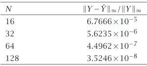
[image:10.498.170.345.247.312.2] [image:10.498.174.324.413.480.2]The exact solution isy(x)=cos(π x/2)and the order of convergence, according to the scheme in [7], isO(hlnh). Numerical results using the new scheme are shown in
Table 4.1. The results show that the order of the convergence of the relative error is about 3.6.
Table4.1. The numerical results for Example4.1.
N Y−Y¯ ∞/ Y ∞
16 6.7666×10⁻⁵
32 5.6235×10⁻⁶
64 4.4962×10⁻⁷
128 3.5246×10⁻⁸
Example4.2. Consider
p(x)=sin π x
2
,
w(x)=1,
g(x, y)=π2 2 sin
π x
2
+cos π x
2
cos π x
2
−y2.
(4.2)
Table4.2. The numerical results for Example4.2.
N Y−Y¯ ∞/ Y ∞
16 3.1548×10⁻⁴
32 4.6984×10⁻⁵
64 7.0243×10⁻⁶
128 1.0413×10⁻⁶
Note that in both examples, the order predicted byTheorem 3.1is at leasth2(lnh)2. Our numerical method achieved higher accuracy for both examples. For the special casep(x)=w(x)=xα, our method is identical to the method constructed in [4] and thus the order ish4. Examples are presented in [4].
Appendix
Some auxiliary lemmas
LemmaA.1. For 0≤a < x≤b≤1, x
a
w(t)dt b
x
p−1(t)dt≤ x
a b
t
p−1(τ)dτ
w(t)dt. (A.1)
Proof. The inequality follows from
x
a
w(t)dt b
x
p−1(t)dt= x
a b
x
p−1(τ)dτ
w(t)dt
≤ x
a b
t
p−1(τ)dτ
w(t)dt,
(A.2)
sincep≥0.
LemmaA.2. Let
Ux−(t)= t
x−δp
−1(τ)dτ x
x−δp
−1(τ)dτ
, Ux+(t)= x+
t p
−1(τ)dτ x+
x p
−1(τ)dτ ,
Ux(t)=
Ux−(t), x−δ≤t≤x, Ux+(t), x≤t≤x+ .
(A.3)
Then,
x+
x−δUx(t)w(t)dt 1
xp
−1(t)dt≤2 x+
x−δ 1
t p
−1(τ)dτw(t)dt (A.4)
Proof. Note that x+
x−δUx(t)w(t)dt 1
xp
−1(t)dt=x x−δU
−
x(t)w(t)dt x+
x p −1(t)dt
+ x+ x U + x(t)w(t)dt x+ x p −1(t)dt
+ x+
x−δUx(t)w(t)dt 1
x+ p
−1(t)dt.
(A.5)
For the first integral of (A.5), sinceUx−≤1, it follows fromLemma A.1that x
x−δU −
x(t)w(t)dt x+
x p
−1(t)dt≤ x
x−δw(t)dt x+
x p −1(t)dt
≤ x
x−δ x+
t
p−1(τ)dτ w(t)dt ≤ x x−δ 1 t
p−1(τ)dτ
w(t)dt.
(A.6)
Similarly, for the third integral of (A.5), we have x+
x−δUx(t)w(t)dt 1
x+ p
−1(t)dt≤x+
x−δw(t)dt 1
x+ p −1(t)dt
≤ x+
x−δ 1
t
p−1(τ)dτ
w(t)dt.
(A.7)
For the second integral of (A.5), it follows from the definition ofUx+(t)that
x+
x
Ux+(t)w(t)dt x+
x
p−1(t)dt= x+ x x+ t p
−1(τ)dτ x+
x
p−1(τ)dτ w(t)dt x+ x
p−1(t)dt
= x+
x
x+
t p
−1(τ)dτw(t)dt
≤ x+
x 1
t
p−1(τ)dτ
w(t)dt.
(A.8)
The results follow from (A.6), (A.7), and (A.8).
Acknowledgment. The authors are grateful for the financial support provided by King Fahd University of Petroleum and Minerals.
References
[1] I. T. Abu-Zaid and M. A. El-Gebeily,A finite-difference method for the spectral approxima-tion of a class of singular two-point boundary value problems, IMA J. Numer. Anal. 14(1994), no. 4, 545–562.
[3] M. M. Chawla, S. McKee, and G. Shaw,Orderh2method for a singular two-point boundary value problem, BIT26(1986), no. 3, 318–326.
[4] M. M. Chawla, R. Subramanian, and H. L. Sathi,A fourth order method for a singular two-point boundary value problem, BIT28(1988), no. 1, 88–97.
[5] P. G. Ciarlet, F. Natterer, and R. S. Varga,Numerical methods of high-order accuracy for singular nonlinear boundary value problems, Numer. Math.15(1970), 87–99. [6] K. Deimling,Nonlinear Functional Analysis, Springer-Verlag, Berlin, 1985.
[7] M. A. El-Gebeily and I. T. Abu-Zaid,On a finite difference method for singular two-point boundary value problems, IMA J. Numer. Anal.18(1998), no. 2, 179–190. [8] M. A. El-Gebeily, A. Boumenir, and M. B. M. Elgindi,Existence and uniqueness of solutions of
a class of two-point singular nonlinear boundary value problems, J. Comput. Appl. Math.46(1993), no. 3, 345–355.
[9] P. Jamet,On the convergence of finite-difference approximations to one-dimensional sin-gular boundary-value problems, Numer. Math.14(1969/1970), 355–378.
[10] J. M. Ortega and W. C. Rheinboldt,Iterative Solution of Nonlinear Equations in Several Variables, Academic Press, New York, 1970.
K. M. Furati: Department of Mathematical Sciences, King Fahd University of
Petroleum and Minerals, Dhahran31261, Saudi Arabia
E-mail address:[email protected]
M. A. El-Gebeily: Department of Mathematical Sciences, King Fahd University of
Petroleum and Minerals, Dhahran31261, Saudi Arabia