The Business Intelligence as a Service in the Cloud

Citation:

Chang, V (2014) The Business Intelligence as a Service in the Cloud. Future Generation Computer Systems, 37. 512 - 534. ISSN 0167-739X DOI: https://doi.org/10.1016/j.future.2013.12.028

Link to Leeds Beckett Repository record: http://eprints.leedsbeckett.ac.uk/220/

Document Version: Article

The aim of the Leeds Beckett Repository is to provide open access to our research, as required by funder policies and permitted by publishers and copyright law.

The Leeds Beckett repository holds a wide range of publications, each of which has been checked for copyright and the relevant embargo period has been applied by the Research Services team.

We operate on a standard take-down policy. If you are the author or publisher of an output and you would like it removed from the repository, please contact us and we will investigate on a case-by-case basis.

T

I

S

C

1. School of Computing and Creative Technologies, Leeds Metropolitan University, Leeds, UK.

2. School of Electronics and Computer Science, University of Southampton, Southampton, UK.

[email protected]

Abstract

Limitations imposed by the traditional practice in financial institutions of running risk analysis on the desktop mean many rely on models which assume a “normal” Gaussian distribution of events which can seriously underestimate the real risk. In this paper, we propose an alternative service which uses the elastic capacities of Cloud Computing to escape the limitations of the desktop and produce accurate results more rapidly.

The Business Intelligence as a Service (BIaaS) in the Cloud has a dual-service approach to compute risk and pricing for financial analysis. In the first type of BIaaS service uses three APIs to simulate the Heston Model to compute the risks and asset prices, and computes the volatility (unsystematic risks) and the implied volatility (systematic risks) which can be tracked down at any time. The second type of BIaaS service uses two APIs to provide business analytics for stock market analysis, and compute results in the visualised format, so that stake holders without prior knowledge can understand. A full case study with two sets of experiments is presented to support the validity and originality of BIaaS. Additional three examples are used to support accuracy of the predicted stock index movement as a result of the use of Heston Model and its associated APIs.

We describe the architecture of deployment, together with examples and results which show how our approach improves risk and investment analysis and maintaining accuracy and efficiency whilst improving performance over desktops.

Key Words

Heston Model Simulations; Heston Model; Business Intelligence as a Service (BIaaS); Calibration; APIs for stock index; Visualisation in the Cloud; SaaS in the private cloud.

1.

1. Introduction

1.1

Background

David X Li improved concepts implemented by financial services and modelled ‘credit derivatives’ to calculate collateralised debt obligation (CDO), which is a type of structured asset-backed security (ABS) with multiple series issued by special purpose entities for debt obligations including bonds and loans. Li allowed his model to get yields of a corporation’s bonds or the prices of the new credit swaps to model the ‘survival time’ of an individual corporation (the time until it defaults). Li resolved this issue by introducing ‘copula function’ that he learned in statistics. Copula function is commonly used in mortgage lending concept to calculate the impacts of defaults due to deaths of one of the spouses [2]. Copula function can calculate set of marginal functions (to specify the probability that the wife will die before a given age, and separate function that specifies that the husband will die at or before another age) to form the joint or ‘multivariate’ distribution function (to specify the probability that the wife will die before a given age AND the husband will die at or before another age). This is one of the fundamental errors that Li has implemented, since probability for both events to happen is different from one event to happen and results can be varied widely in extreme conditions.

Li then combined a popular financial software, CreditMetrics, and Copula function together to establish “Gaussian copula” model, which has been used by the finance industry since 1997 [1]. The “Gaussian copula” model is often called as CDO solution, since it is a term easily understood by the finance sector. By combining both approaches, finance sector could enjoy benefits from both sides – Gaussian’s simplicity and familiarity and copula’s unified and easy-to-use approach. Gaussian copula model allowed analysts to buy a pool of bonds or loans, raising their money to do so by selling investors’ securities claimed on the cashflow generated from the pool. The drawback for this approach is the assumption that correlation stays low. If correlation goes too high, the holders of the highest investment were at risks, and there was no detailed way to compute the extent of volatility in such extreme conditions [1], since the model takes assumption on the ‘bright side’ of the trading due to simplification of “Gaussian copula” model to compute complex financial derivatives, prices and volatility.

Li then developed his final version of software called CDO Evaluator, which became more and more popular amongst quantitative developers and investment banks. There were a few reasons according to MacKenzie and Spears [1] and their interviews with experts and developers working in financial services. Firstly, developers needed not to think of many variables which are time-consuming to obtain. Secondly, they could possibly avoid using Monte Carlo simulations that took overnight and the weekend to run through all simulations and perform exhaustive testing of financial derivatives. Thirdly, it was easier to understand the problems, since there were fewer variables to know. Fourthly, it was also easier to communicate with other teams. Financial problems and derivatives were difficult to understand and even within teams with different skills and focus, communications were not easy or lengthy. The use of concepts of “Gaussian copula” model and the CDO Evaluator could ease the level of difficulties during communications. Fifthly, developers found it easy to reproduce Li’s concepts due to the simplicity of the model and the problem. Sixthly, his software was backed by some leading quantitative developers at that time, and had widespread use in investment banks.

1.2

Business Intelligence as a Service (BIaaS) in the Cloud

which are currently missed. However, factors such as accuracy, speed, reliability and security of financial models and their attendant costs must be considered [4]. Public clouds are not suitable due to privacy and data ownership issues [5]. A hybrid cloud could be used but this requires implementation of security technologies which are not the focus of our research. Private clouds are the obvious choice for the financial sector and also relevant to our objective.

The term “Business Intelligence” refers to a set of methods, processes, architectures and technologies that can process and transform collected datasets into meaningful and useful information for business purposes, and often used in business-critical servers, applications and services. Advanced simulations and processing in financial computing such as derivatives, stock analytics and financial software are part of Business Intelligence (BI), which aims to simplify the complexity of datasets and presents them with information for IT strategies and operational activities [6]. Daily activities performed by investment banks can be used by BI systems as an alternative, and another additional advantage is that BI systems can integrate with other technologies such as Cloud Computing to offer more added values to organisations [6, 7, 8]. There are two examples here to illustrate the added values of using BI systems in the Cloud. Firstly, Xu [7] designed and developed Cloud BI systems for manufacturing, and demonstrated how Cloud BI can transform the way that manufacturing was used to work. Cloud BI allowed different machines to work collaboratively and efficiently. Secondly, Marston [8] explained the added values of Cloud BI systems for business perspective and they demonstrated examples on how organisations could get different levels of contributions by using Cloud services such as Cloud BI services. These examples acknowledge the benefits of adopting BI in the Cloud for improved technical and business perspectives, thus, a hybrid solution of integrating BI in the Cloud is another motivation for this paper.

We propose and describe Business Intelligence as a Service (BIaaS) which is a Cloud based service designed to improve the accuracy and quality of both pricing and risk analysis in financial markets, compared with traditional desktop technologies. BIaaS is a type of Software as a Service (SaaS) with the emphasis on how the application offers quality services in private cloud environments. This is important because incorrect analysis leads to excessive risk taking which may then lead to financial losses, damage to business credibility or destabilised markets. We illustrate its use with an example which shows price and risk assessments for investments such as stocks and shares or financial derivatives in the context of different levels of volatility, maturity and risk free rates.

BIaaS has the dual-service approach to address the following challenges:

1. Compute the risks and asset prices, and computes the volatility which can be tracked down at any time.

2. Performing a sufficiently high number of simulations in acceptable time.

2.

2. Problems with existing Gaussian copula modelling and our proposal

This section is aimed at describing the problems caused by Gaussian copula modelling, a model widely adopted by financial services and investment banks to calculate the lending. It starts with backgrounds, the process of getting popularity and explanations about the problems associated with the model.

2.1

Simplicity at the expense of accuracy and performance

However, Li’s contributions to the finance industry were known as “receipt to disaster” after the financial crisis since 2008. The model underestimated the probability of the risks and did not have any measure to counter the risks when they began to take an immediate effect. Several assumptions he made his model did not work in extreme conditions [1]. His model could work on the desktop and results could be calculated for an acceptable amount of time. By taking simplification of Li’s model, financial services could run their services and get the results quickly. This can avoid the need to run days and hours of Monte Carlo simulations. However, risks are not properly checked as a consequence. His model took the simplicity and ease-of-use at the expense of the risk modelling and controls [1]. Li also admitted his weakness of the model and wrote: “The current copula framework gains its popularity owing to its simplicity....However, there is little theoretical justification of the current framework from financial economics....We essentially have a credit portfolio model without solid credit portfolio theory” [9]. However, we argue that it is unprofessional to take false assumption and encourage users to take simplicity due to convenience. It is important to run models properly without sacrificing the quality of results but also offer a prompt services without the need of running simulations for hours and days.

2.2

BIaaS Private Cloud is the solution other than desktop

Running simulations on desktop clearly need much longer time and a smart way of performing a high number of simulations with a short time is required. The use of Cloud Computing techniques and technologies can play an important role to optimise the speed and also allow more vigorous tests and simulations are performed. The BIaaS private cloud is designed and deployed to ensure all calculations of pricing and risks are as accurate as possible and also can be computed within seconds and minutes. This can help financial services to perform thorough testing without compromising to run simpler model which does not take risks (happened in extreme condition of probability of 2% and lower) seriously. Different models and scenarios of risks models will be presented.

2.3

BIaaS – requirements and the need to rectify errors left by Gaussian

copula model

It becomes important for computer scientists to develop better models to improve such a situation. Better ways to calculate pricing and risks, rectify errors and perform accurate and fast simulations are highly desirable. Requirements for our BIaaS are thus as follows:

1. Based on the reputable models – Our BIaaS adopts reputable models including the Heston Model (which includes the Wiener process and the Stochastic Volatility) and the Visualisation APIs to compute the best pricing and risks for different scenarios.

3. Accuracy – our BIaaS can compute pricing and risk values to several decimal places and also calculate its mean, lower and upper range to get our results as accurate as possible.

4. BIaaS should not just limit its operations on desktop or a particular platform but on different types of Clouds and desktop.

Results or discussions in other sections of the paper will refer back to here to explain how other development can fulfil requirements for BIaaS.

3.

3. Outline of BIaaS and Methods used by BIaaS

Gaussian copula models are used in financial modelling and many banks’ mathematical models assume normal (Gaussian) distributions of events and may underestimate risks in real financial markets [10]. Moreover, these models make assumptions about market behaviour which may not always be true with the result that the models can fail to detect risks, as highlighted by the financial crisis in 2008. To address this alternative, non-Gaussian financial models are needed. Various studies conclude that modelling of financial markets needs to be addressed in two stages; one for pricing and another for risk analysis [1, 11]. This means a more suitable model is required for large-scale of financial analysis. BIaaS is the most commonly adopted and provides data for investors’ decision-making amongst other models [12].

3.1

The Heston Model: fulfilling the first BIaaS requirement

This section explains the suitable model for BIaaS to fulfil the first requirement presented in Section 2.3. BIaaS is derived from mathematical Heston Model and additional APIs and is a computational technique used to calculate risk; the probability of an event or investment happening. BIaaS is based on probability distributions, so that uncertain variables can be described and simulated with controlled variables [12, 13]. BIaaS is suitable to generate data which investors can use when making decisions [10]. When volatility is known, put and call prices can be calculated [14, 15]. Moreover, BIaaS has specific techniques such as Wiener process to compute high-volume of simulations and track the movements of volatility for the computed data.

The Heston Model has a close relationship with Black-Scholes model, since it relaxes the constant volatility assumption in the classical Black-Scholes model by incorporating an instantaneous short term variance process [16]. This means the Heston Model can be used in a more flexible way and is not as theoretical-oriented as the classical Black-Scholes model does. In addition, there are both the Wiener process and the CIR process related to the Heston Model, and their explanation is as follows.

3.2

The Wiener process and the Heston Model

The Wiener process is a continuous-time stochastic process named after Norbert Wiener. It is a standard Brownian motion and can be in mathematics. In applied mathematics, the Wiener process is used to represent the integral of a Gaussian white noise process for electronics engineering, instrument filtering theory and control theory. It can be used effectively in the mathematical theory of finance, in particular the Black–Scholes option pricing model. There are three properties in the Wiener process Wt [15, 17, 18]

1. W0 = 0

2. The function t → Wt is almost surely everywhere continuous

The Wiener process is a stochastic process with independent and stationary increments, which means the motion of a point whose consecutive displacements are independent and random with each other. The Wiener process has Lévy characterisation has continuous martingale with W0 = 0 and quadratic variation [Wt, Wt] = t. This implies that Wt2−t is a martingale.

Here is the description to explain the relationship between Wiener process and the Heston Model, which starts with the mathematical formula first.

The basic Heston model assumes that St, the price of the asset, is determined by a stochastic process [20]

(1)

where , the instantaneous variance, is a CIR process, which is a Markov process with continuous paths defined by the following stochastic differential equation (SDE):

(ν0 =ξ2 , which is > or = 0) (2)

and are Wiener process (i.e., random walks) with correlation ρ dt.

The parameters in the above equations represent the following:

• μ is the rate of return of the asset.

• θ is the long variance, or long run average price variance; as t tends to infinity, the expected value of νttends to θ.

• κ is the rate at which νtreverts to θ.

• ξ is the volatility of the volatility; as the name suggests, this determines the

variance of νt.

All these parameters can be used in calibration to determine their respective values, and is an important process used by other models to validate results in financial analysis. Details will be presented in Section 3.5 for the right type of parameters used, and in Section 8.1 for large-scale experiments for result validation.

If the parameters obey the following condition (known as the Feller condition) then the process is strictly positive [17, 18]

3.3

The CIR process and the Heston Model

Heston model is initially derived from the CIR model of Cox, Ingersoll and Ross [18, 19] for interest rates. CIR process is a Markov process with continuous paths defined by the following stochastic differential equation (SDE) presented by formula (2). The CIR process is used to model stochastic volatility in the Heston model, which aims to resolve a shortcoming of the Black–Scholes model which corresponds to the fact that the implied volatility does tend to vary with respect to strike price and expiry. By assuming that the volatility of the underlying price is a stochastic process rather than a constant, stochastic volatility can make it possible to model derivatives more accurately.

3.4

Runge-Kutta method

The Runge–Kutta method (RKM) is a technique for the approximate numerical solution of a stochastic differential equation (SDE) [15, 18]. RKM can be used to generalise the ordinary differential equation to SDE. The related formulas are as follows.

the Itō diffusion Xsatisfying the following Itō stochastic differential equation [18, 21]

(3)

with initial condition X0 = x0, where Wt stands for the Wiener process, and suppose that we wish to solve this SDE on some interval of time [0, T]. Then the Runge–Kutta approximation to the true solution X is the Markov chain Y defined as follows:

• partition the interval [0, T] into N equal subintervals of width δ = T⁄ N > 0:

• set Y0 = x0;

• define Yn for 1 ≤ n≤ N by

(4)

where

and

ΔWn are independent and identically distributed normal random variables with expected value zero and variance δ. RKM can be used to calculate SDE, which is required by the Heston Model.

3.5

Root-mean square error (RMSE) – the first formulas for calibration

Calibration is used in Business Intelligence in a way that a known observation of the dependent variables is used to predict a corresponding explanatory variable. Systematic approaches are followed based on the adoption of right formulas. There are two associated formulas in regard to calibration. The first formula is the root-mean square error (RMSE) and the second is moving windows (MW) estimate [18, 21].

The root-mean square error (RMSE) is used to measure of the differences between values predicted by a model or an estimator and the values actually observed. RMSE also determines the goodness of fit of the Heston Model presented as follows [18, 21].

n X X

RMSE

n

i obsi modeli

∑

= 1

2 ,

, )

(

(5)

Guillaume and Schoutens [22] explain that parameters in RMSE can be recalibrated every day to new market data, and optimal parameter set can vary significantly on a day-to-day basis. An important goal is to avoid sharp fluctuations of the model parameters. An alternative is to use or restore the time series or market quotes to calculate some of the model parameters. Guillaume and Schoutens [22] explain that parameters ν0 can be remained fixed before calculating the value of volatility index, where (To avoid confusion with n, researchers use θ to differentiate) can be estimated by the following three ways:

1. Historical time series of the volatility: This is a common approach demonstrated by researchers [14, 17, 18, 21].

2. Market quote of the VIX options: VIX is known as the Chicago Board Options Exchange Market Volatility Index, which is a popular measure of the implied volatility of S&P 500 index options [22, 23]. The Moving Window estimate can be used for computation for forecasting of the market index.

3. Another model to deal with fluctuations: Another model and approach is required. A common approach is to use exponentially weighted moving average (EWMA) [22, 23].

In current BIaaS implementation, the first and second objective can be demonstrated to show that BIaaS can compute volatility and calculate the likely movement in the stock index. Referring to Section 2.3, both performances (tracking of volatility) and accuracy can be achieved by the combined approach in the first and two objectives above.

3.6

The Moving Window (MW) estimate and exponentially weighted

moving average (EWMA) - the second and third formulas for calibration

(6)

For this paper, MW is used to compute the forecasted movement in the Heston Model.

On the other hand, exponential weighted moving average (EWMA) estimate the long run variance presented as

(7)

Where (0,1), ti = t0 – (N –i) t and where N is the number of data in the time

3.7

Average absolute percentage error (APE) of the mean price and

aggregated relative percentage error (ARPE) – additional formulas for

calibration

Two additional formulas are useful for validation of results. Average absolute percentage error (APE) of the mean price is a measure of accuracy of a method for constructing fitted time series values in statistics and financial computation [18, 21, 22].

(8)

Calculations by APE may cause a problem. A few of the series with a very high APE might distort a comparison between the average APE of time series fitted with one method compared to the average APE when using another method. To improve on this situation, another model, aggregated relative percentage error (ARPE) is used.

(9)

All the formulas in Section 3.5, 3.6 and 3.7 can utilise parameters (ν0, κ, θ, ξ , ρ) for calibration.

4.

4. The APIs and System Architecture for BIaaS

Section 3 explains all the formulas associated with BIaaS. However, mathematical modelling is not easy to use and analysts need years of training to be sufficiently competent for financial computation. Additional work is then required, including the development of APIs that perform financial computations and only presents the results to the analysts. In order to understand the work behind the scene, this section explains the high-level functionality of BIaaS, the role and functionality of associated APIs and the system architecture in order to perform experiments for Section 5, 6 and 7.

4.1

Two major services to offer

For the demonstration for this paper, experiments are running at two sites starting from Southampton, and the processing take place mainly at ULCC in London. Figure 15 in the Appendix shows the deployment where the details of hardware implementations are described in Section 5. Two different Cloud services are developed and their descriptions are as follows:

• Business Analytics as a Service (BAaaS): After analysing the numerical computation of volatility and pricing, the next step is to compute them as a Business Analytic. This makes the analysis much easier and the stakeholders can understand. After the processing of HVPaaS completed in Southampton, results are sent to Greenwich and ULCC in London, where both sites can process BAaaS. ULCC has better platforms and can produce a large-scale of processing than Greenwich.

Details for each service will be presented in Section 6 and 7 respectively. We first present how each service works in their system architecture and then how the two services can work together in the collaborative Cloud environment.

4.2

The role of the Application Programming Interfaces (APIs) for BIaaS

Formulas and theories behind the Heston Model, the Wiener process, the CIR process and RKM can be complex and not easy to be interpreted correctly in a way appealing to stake holders and investors. It is important for Cloud services to be easy to use as usability is a key criteria for successful Cloud delivery [24, 25]. In this research, APIs are used to bridge the gap between the complexity of the mathematical models and the good delivery of Cloud services. The emphasis is on how these APIs can be used, the results and benefits offered by the private cloud development for financial services research. Section 4.4 and 4.5 will describe the functionality of five APIs. Section 6 and 7 will describe the detailed usage scenarios for these five APIs.

4.3

System Design and Architecture

Figure 1: System Design and Architecture for BIaaS in Southampton and London Private Cloud sitting on top of NGN

4.4

Three APIs for the Heston Model

There are three APIs developed for the Heston Model to calculate the implied volatility. The Heston Model can use all of the Wiener process, the CIR process and Runge–Kutta method to achieve this as explained earlier. Each API can be used as a one-line command line. The APIs and functionality for each API are as follows.

1. ItoProcess API - this uses the Wiener process to launch stochastic process and calculate key variables for the Heston Model.

2. BlockRandom API – this is relevant to the Runge–Kutta method to compute stochastic differential equation for the Heston Model.

3. CovarianceFunction API – this is relevant to the Wiener process mainly and the CIR process to treat any process as a random process so that no input data is required. However, CovarianceFunction is used when key variable are known and the volatility is calculated. This means there is a higher level of confidence in those key values prior using CovarianceFunction.

There is an optional API, Plot, which computes all numerical results and displays them as 3D Visualisation. This allows stakeholders to understand it more easily.

Results are saved in numerical formats readable by each API service and then passed onto the next API. Service 2 is BAaaS which is itself comprised of two APIs. Results from the last API of first service in Southampton have two options. The first option is to report results in numerical formats, which can be interpreted by scientists and experienced data analysts. However, if such analysis is difficult to interpret, additional APIs are required to simplify the complexity for stakeholders. For the demonstration for this paper, BIaaS takes on the second option, which allows the result from “CovarianceFunction” API to pass onto the first API of BAaaS in London.

4.5

APIs for the Business Analytics Visualisation

APIs for visualisation are useful to present risks and asset prices in real-time. Visualisation can be used for purposes such as the review of the previous performance and review of the

Each dot represents a step/sub-service

Virtualised applications Service 1 Service 2

SaaS 1

PaaS 1

IaaS 1

SaaS 2

PaaS 2

IaaS 2 Choose to get results

Input 1

Results are sent to other VMs

Service N (Futurework) Input 2 (if necessary)

Data exchang

SaaS N

PaaS N

current performance, particularly for the stock market analysis. There are two APIs available for the visualisation service and their function is described briefly as follows.

1. FinancialData API – this allows the BIaaS Cloud to obtain financial data from Google Finance and have all the major stock market data, particularly the US and UK stock exchange data.

2. TradingChart API – this allows the financial data to be presented in the trading chart format similar to the visualisation services offered by London Stock Exchange and Thomson Reuters. There are two additional functions, “SimpleMovingAverages” and “BollingerBands”,which corresponds to the use of MW model to compute forecasted movement. “TradingChart” is the API to demonstrate both models (Heston and Financial data) can work together to deliver an integrated service.

Details for the analysis will be available in the Section 6 and 7.

4.6

Operation of BIaaS

Referring to Figure 1, results are saved in numerical formats readable by each API service and then passed onto the next API. This can ensure the entire service to operate as an integrated service. The dual-service approach of operating BIaaS includes:

1. Risk simulation service using BIaaS: This includes calculating the volatility and the asset prices, and their real-time numerical values. ItoProcess, BlockRandom, CovarianceFunction (based on the Heston Model) and Plot APIs are developed to support this function.

2. 3D Visualisation of pricing and volatility – The synchronised asset prices and volatility is computed and presented in 3D Visualisation and in a way that stake holders can understand without prior knowledge. FinancialData and TradingChart APIs are developed to support this function. FinancialData uses Google Finance and the Heston Model for financial computation.

3. Trading analytics: BIaaS offers the computation of the trading analytics. Although TradingChart is the main API for this functionality, it does require support from all other APIs to deliver this service.

5.

5. Deployment for the experiments

This section describes the hardware, architecture and deployment scenarios used for performing experiments and simulations for BIaaS. Section 4.1 explains the hardware set up, section 4.2 describes the deployment scenario and section 4.3 presents the architecture.

5.1

Hardware used for experiments and benchmarks

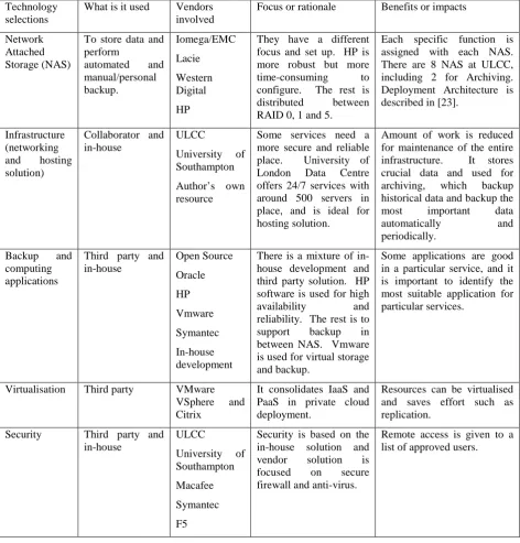
Table 1: Selections of Technology Solutions

Technology selections

What is it used Vendors involved

Focus or rationale Benefits or impacts

Network Attached Storage (NAS)

To store data and perform automated and manual/personal backup. Iomega/EMC Lacie Western Digital HP

They have a different focus and set up. HP is more robust but more time-consuming to configure. The rest is distributed between RAID 0, 1 and 5.

Each specific function is assigned with each NAS. There are 8 NAS at ULCC, including 2 for Archiving. Deployment Architecture is described in [23].

Infrastructure (networking and hosting solution) Collaborator and in-house ULCC University of Southampton Author’s own resource

Some services need a more secure and reliable place. University of London Data Centre offers 24/7 services with around 500 servers in place, and is ideal for hosting solution.

Amount of work is reduced for maintenance of the entire infrastructure. It stores crucial data and used for archiving, which backup historical data and backup the most important data automatically and periodically.

Backup and computing applications

Third party and in-house Open Source Oracle HP Vmware Symantec In-house development

There is a mixture of in-house development and third party solution. HP software is used for high

availability and reliability. The rest is to

support backup in between NAS. Vmware is used for virtual storage and backup.

Some applications are good in a particular service, and it is important to identify the most suitable application for particular services.

Virtualisation Third party VMware

VSphere and Citrix

It consolidates IaaS and PaaS in private cloud deployment.

Resources can be virtualised and saves effort such as replication.

Security Third party and in-house ULCC University of Southampton Macafee Symantec F5

Security is based on the in-house solution and vendor solution is focused on secure firewall and anti-virus.

Remote access is given to a list of approved users.

London Data Centre has advanced Cloud and parallel computing infrastructure and network attached storage (NAS) service. In total it has CPUs totalling 30 GHz, 60 GB of RAM and 12 TB of disk space in place. Experiments performed in this environment get the best benefit of advanced optical fibre networking. There are two servers at London Greenwich, with a total of 9 GHz CPU and 20 GB RAM. The two servers at University of Southampton both have 6.0 GHz and 16 GB RAM. For the home cluster, the total hardware capability is 24.2 GHz CPU and 32 GB RAM.

infrastructure and platform at ULCC to provide reliable and accurate services. Design and Deployment is based on project requirements and their research focus. Selections of Technology Solutions are essential for Cloud Storage development as presented in Table 1.

5.2

Motivation for performing experiments for BIaaS

Business Intelligence as a Service (BIaaS) can also be used independently but it needs manual input of data for processing if that is the case. In this paper, the focus is to demonstrate that BIaaS in the Cloud can be delivered as an integrated service consisting of two different services. The first service is Heston Volatility and Pricing as a Service (HVPaaS) to process stochastic equations and present the calculated implied volatility and pricing. The second service is Business Analytics as a Service (BAaaS) to present financial data and analysis in a collaborative and easy-to-understand way. This makes integrations of two services useful for BIaaS development from both development and enterprise points of view. Technical developers can find that technical capabilities can allow them to compute two different types of business intelligence modelling once rather than twice. The business benefits for the enterprise is the reduction of time and cost to deliver services, which means the enterprise only pay the service once rather than twice to different service providers. Integrating both services requires the following:

• Results from the end of HVPaaS and the end of each API need to be saved as text (or numerical format) passed to the next step, allowing results from each API to be passed onto the next.

• Streamlining both services as a single process and ensure both are completed in one go rather than as two separate services.

The experiments are performed using a private cloud located in Southampton, distributed between two sites; two high performance servers with multiple VMs located at University of Southampton and two clusters of eight servers with VMs located at the lead author’s home. All are connected to form a private cloud.

5.3

Preliminary set up to minimise risks

There are risks that can affect the performance of experiments. They mainly include synchronisation, network traffic control and library dependency. Risk-control rate is the rate to control risk of running experiments. The target is to maintain the incomplete API processing within 1%. Risk-control rate must be managed carefully and this can be achieved by the following steps.

• Synchronising all experiments: This can ensure experiments to London and Southampton start at the same time, and it makes the management of risk-control rate once rather than twice per experiment. Or all experiments are running in London, and all experiments start simultaneously.

When the upload network speed reduces, checks will be carried out to see whether network speed is slow at all sites, particularly within ULCC. If there is more than one place having slower network speed and are within 4 Mbps difference to each other, experiments can continue. But if there is only one place with a slower network, then the entire experiment will halt until the network upload time is back to normal and within 4 Mbps of each other.

• Library or software dependency: It is useful to check with any existing API or tools that have library or software dependency. If there is, all updates will take place and the system reboot will ensure there is no any influence on the execution time and processing of APIs.

5.4

The execution time for running BIaaS dual-service in the local

environment

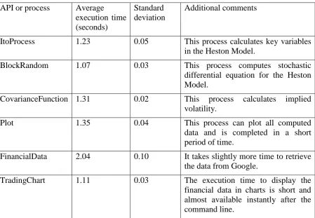
This section describes the execution time for using BIaaS services, with the objective to demonstrate that BIaaS is efficient, quick and accurate to produce good-quality results. The first step is to test the execution time in each API in the local environment where risk concerning with performance of experiments is not a concern. It can be done on either server 2 at the University of Southampton or 1 of HPC servers at ULCC. Results are running one hundred times to get the average execution time. The standard deviation is always 0.10 and below and p value is less than 0.005 presented in Table 2.

Table 2: The execution time for each API or process in the local environment (p < 0.005)

API or process Average execution time (seconds)

Standard deviation

Additional comments

ItoProcess 1.23 0.05 This process calculates key variables

in the Heston Model.

BlockRandom 1.07 0.03 This process computes stochastic

differential equation for the Heston Model.

CovarianceFunction 1.31 0.02 This process calculates implied volatility.

Plot 1.35 0.04 This process can plot all computed

data and is completed in a short period of time.

FinancialData 2.04 0.10 It takes slightly more time to retrieve the data from Google.

TradingChart 1.11 0.03 The execution time to display the

5.5

The execution time for running BIaaS dual-service between

Southampton clusters

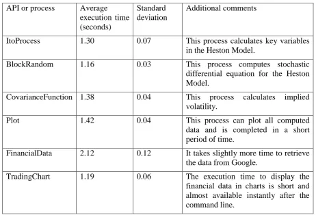
There are two sites that can process BIaaS fully, and one site is located at the University of the Southampton (server 2) and one site is at ULCC (HPC servers) according to Figure 15. There are two additional experiments required. The first experiment is to make a request from server 1 to server 2 within the University of Southampton. The physical location between server 1 and 2 is about 100 meters and the network upload speed is 1 Gbps during the time experiments took place. The second experiment is to make a request in Southampton and process in ULCC in London and will be presented in the next section. The aim is to test the execution time while network speed becomes an influential factor. Results are running one hundred times to get the average execution time. The standard deviation is always 0.12 and below and p value is less than 0.005 presented in Table 3.

Table 3: The execution time for each API or process in the local environment (p < 0.005)

API or process Average execution time (seconds)

Standard deviation

Additional comments

ItoProcess 1.30 0.07 This process calculates key variables

in the Heston Model.

BlockRandom 1.16 0.03 This process computes stochastic

differential equation for the Heston Model.

CovarianceFunction 1.38 0.04 This process calculates implied volatility.

Plot 1.42 0.04 This process can plot all computed

data and is completed in a short period of time.

FinancialData 2.12 0.12 It takes slightly more time to retrieve the data from Google.

TradingChart 1.19 0.06 The execution time to display the

financial data in charts is short and almost available instantly after the command line.

Although the average execution time is slightly higher than running in local environment, the processing of API and the delivery of services still short execution time.

5.6

The execution time for running BIaaS dual-service between

Southampton and ULCC London clusters

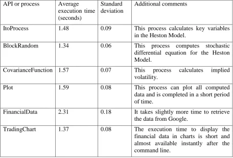
Table 4: The execution time for each API or process in the local environment (p < 0.005)

API or process Average execution time (seconds)

Standard deviation

Additional comments

ItoProcess 1.48 0.09 This process calculates key variables

in the Heston Model.

BlockRandom 1.34 0.06 This process computes stochastic

differential equation for the Heston Model.

CovarianceFunction 1.57 0.07 This process calculates implied volatility.

Plot 1.59 0.08 This process can plot all computed

data and is completed in a short period of time.

FinancialData 2.31 0.18 It takes slightly more time to retrieve the data from Google.

TradingChart 1.37 0.08 The execution time to display the

financial data in charts is short and almost available instantly after the command line.

Results show that despite of the network speed and physical distance difference, the difference in execution time is still small comparing execution time in Table 3. The APIs are designed not entirely to rely on network speed for service delivery and network speed is useful to send back results from server to the client. The emphasis of the API is designed to use mathematical formulas for computation.

Additional demonstrations and tests will be described in Section 6 and 7 based on the hardware infrastructure presented in this section.

6.

6. The first service of BIaaS: Realisation of Heston’s Stochastic Volatility

Model

This section describes the first stage of BIaaS, focusing on Heston’s Stochastic Volatility model. There are two ways of using this service. The first way is to calculate the volatility and compute them in 3D Visualisation. The focus is to investigate the movement of the volatility with the respect of time and percentage of profitability. This requires calculating the Stochastic Volatility to generate all possible cases and data points. The use of BIaaS then presents all these calculations as 3D Visualisation. There are two scenarios used to demonstrate this service.

6.1

Tracking prices and volatility simultaneously

unsystematic risks, which can be managed and minimised. The implied volatility belongs to the first type of the risks. There are still ways to reduce the impacts caused by the implied volatility. This is an important aspect for risk engineering as innovative ways should be explored to detect the likelihood of extreme events to happen, and also recommendation to reduce the damaging impacts when they happen [1, 32].

Calculations of the implied volatility can be done by applying the Heston Model, which has the advantage over the Black Scholes Model (BSM) to calculate the implied volatility for normal and extreme conditions. The Heston Model uses the Stochastic Volatility (in the CIR process) to calculate the implied volatility as discussed in Section 3.3.

This section describes how to track prices and volatility simultaneously which has become more important for the finance sector [33]. As discussed in Section 4.4, an API is required for the Heston Model. We have an API known as “ItoProcess” to use the Wiener process to help to calculate key variables (x and t, see the IToProcess API) for the Heston Model, and later on can compute the implied volatility when values for key variables are known. The API can be used like a command-line as follows.

ItoProcess[sdeqns, expr, x, t, wdproc]

This command represents an Ito-process specified by a stochastic differential equation “sdeqns”, output expression “expr”, with state x and time t, driven by w following the process “dproc”.

ItoProcess[..., {x, x0}, {t, t0}]

This is another command uses initial condition x(t0) = x0.

The implementation of this model requires the following procedures:

Step 1: Define the “IntoProcess” and use a correlated 2D Wiener process to define a Heston Model by SDEs. It looks like:

(a)

Step 2: Use a stochastic Runge-Kutta method to simulate the Heston model for Year 2012. It looks like:

td=BlockRandom[SeedRandom[2012];

RandomFunction[hm/.{µ→0,κ→2,θ→1,ξ→1/2,ρ→

-1/3,Subscript[s,0]→25,Subscript[r,0]→1.25},{0,1,0.005},6,Meth

od→"StochasticRungeKutta"]]; (b)

These two steps calculate key values and then compute for the Heston Model.

• Collect computed data in (b).

• Use a specific plotting function to plot the computed data (one for asset prices and one for volatility). Specify any additional input values for asset prices and volatility.

• Make both visualised results on the same row.

By doing so, the Heston Model can present both asset prices and volatility. The x-axis is the time for up to 1 year and is the same for both assets and volatility. The higher the volatility is, the less stable (higher risk) that the asset is liable to. The asset price is its market price with the respect with time. The Heston Model allows tracking both prices and volatility simultaneously for the investor’s stock option in 2012. See Figure 2.

0.2 0.4 0.6 0.8 1.0

10 20 30 40 50 60

Price of the asset

0.2 0.4 0.6 0.8 1.0

0.5 1.0 1.5

Volatility of the asset

Figure 2: Tracking both prices and volatility simultaneously for a chosen stock in 2012

6.2

Calculations of the implied volatility and the API

As discussed in Section 4.4, an API is required for the Heston Model. We have an API known as “ItoProcess” to use the Wiener process to help to calculate key variables (x and t, see the ItoProcess API) for the Heston Model, and later on can compute the implied volatility when values for key variables are known. The API command-line is the same as described in Section 6.1, which already calculates the volatility (unsystematic risks, which can be reduced) and asset prices for a chosen stock. In this section, we aim to calculate implied volatility, which is classified as the systematic risks which cannot be controlled. The difference between implied volatility and volatility is that one is systematic and the later is the unsystematic risk. Apart from “ItoProcess”, another command-line oriented API is “Covariance”, and its usage is explained as follows.

Covariance[dist, i, j]

This command provides the covariance for the multivariate symbolic distribution dist.

The implementation of this model requires the following procedures:

Step 2: Use CovarianceFunction

CovarianceFunction[proc,s,t];

This step calculates the required values for key variables, s and t, and have generated computed data.

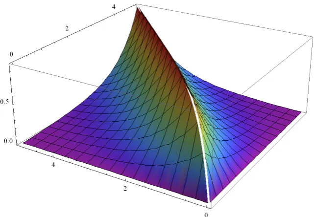
Step 3: Similar to Section 6.1, this step collects computed data for s and t and plots them. Calculations for the implied volatility by the Heston Model are in Figure 3, which can be rotated for 90 degrees as shown in Figure 4.

Figure 3: Calculations of the implied volatility in the Heston Model (original)

Figure 4: Calculations of the implied volatility in the Heston Model (90 degrees)

x-axis: Risk-free rate (0-5%) y-axis: the implied volatility (0 to 1, 1 as the maximum value) z-axis: maturity period (0-5 years)

Low implied volatility (less ‘risky’)

Implications from results:

Both figures show that the implied volatility can reach its peak value at 1 (100%) at any period between the time of investment and four years from the investment, and also between risk-free rates between 0% and 5%. The shape of the modelling results look like a mountain centred between two plains – with higher levels of grounds towards the middle of Figure 3. This means that

• When the risk-free rate is low, it is very likely to get a high implied volatility at a short period of time. When the risk-free rate is improved to 4 and above, it allows the investment to hold on a longer period before the rise of the implied volatility.

• The implied volatility can be nearly at zero: (a) if the risk-free rate is high (5%) but the stock has to be sold within two years, or (b) the stock has to be sold at the end of four years with the risk-free rate is equal to zero. However, Figure 3 (original model) still confirms the option (a) is better as the option (b) needs a longer waiting period after going through a phase of high implied volatility.

Risk visualisation can help investors and analysts to identify when and how risks will be at the peak and the ideal period to avoid higher risks. This provides them useful information for their investment, such as the ideal times to sell or buy stocks due to the change of implied volatility, risk-free rate and time.

7.

7. The second service of BIaaS: Business analytics of stock market

performance

This section is aimed to describe the benefits the business analytics of stock market performance, which enabled by two APIs and belongs to the second type of services offered by BIaaS. Business analytics uses two APIs to enhance the visualisation of existing service and also allow analysts to obtain any stock market analysis. There are also demonstrations for how to use commands lines offered by these two APIs.

7.1

Two Visualisation APIs used as command lines

As explained in Section 4.5, two APIs, “FinancialData” and “TradingChart”, are used to allow analysts and computer scientists to compute financial data to be presented in Visualisation. The focus for this paper is not to discuss what makes these two APIs but how they can be used to maximise the benefits of adopting BIaaS services.

• FinancialData – this command can capture financial data from Google Finance and make data to be understood by the private cloud to be ready for data computation and analysis. It follows the command-line approach which allows users to provide one sentence of line of code to obtain the data.

The usage scenario for the command line includes the followings:

FinancialData["name", {start, end, period}]

This command provides a list of dates and prices for the specified periods lying between start and end.

This command provides a list of dates and values of a property for a sequence of dates or periods.

• TradingChart – this command can compute the data obtained from “FinancialData” command and present them in a way similar to software provided for London Stock Exchange (LSE). Investors can see business analytics of their selected stock.

The usage scenario for the command line includes the followings:

TradingChart[{"name", daterange}]

This command makes a financial chart for the financial entity over a specific range of data.

TradingChart[{...}, {ind1, ind2, ...}]

This command makes a financial chart with indicators, which provides additional analytics functions such as plots and micro analysis.

There is a scenario in the next section to explain how all these commands can work to deliver a solution.

7.2

A scenario to explain how Visualisation works

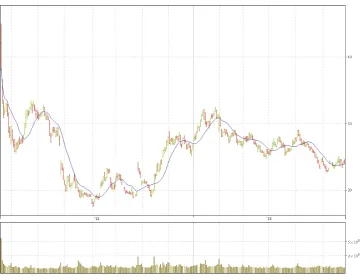
This is a scenario to explain how to obtain the financial analytics computed by the private cloud. For example, an analyst would like to find out the stock market performance for Facebook (FB) for the past thirteen months after its initial public offerings (IPOs) between mid-May 2012 and the end of June, 2013. The command line is

data = FinancialData["FB", "OHLCV", {{2012, 5, 18}, {2013, 6, 25}}];

This command can obtain the data from Google Finance and get data ready for “TradingChart” computation. “OHLCV” means open, low, high, close and volume for the selected stock, which can be obtained from Google Finance to be presented for FinancialData.

TradingChart[data]

Figure 5: Trading chart for Facebook since its IPOs

The next step requires analytics of its recent stock market performance, which means the focus is within the most recent three to four months.

TradingChart["FB", {"Volume", “RelativeStrengthIndex”}]

This command can provide business analytics for FB, which includes

• displaying trading volume for FB;

• displaying Relative Strength Index for FB;

• offering R-squared values, which are used to determine how fit the data is to the overall plot, and is between -1 (rare) and 1. The higher the value, the closer the data is to the overall plot.

• calculating beta, which represents systematic risk value.

Figure 6: Trading chart for Facebook with business analytics

7.3

Tests for accuracy for a particular time period

Section 2 describes the problem faced by the finance industry and accuracy in business analytics is important to ensure results have a high quality and are very close to the actual values in asset prices and risks. There are two types of tests to be performed, and each test is designed for each type of BIaaS service. The second type of BIaaS services is easier to test since it retrieves data from Google Finance, and the output from “TradingChart” can compare results with London Stock Exchange, and also Yahoo UK Finance. Results are exactly the same and thus have 100% accuracy. The first type of BIaaS services can be tested with the description as follows.

• Calculate all values for asset prices, volatility, implied volatility and risk-free rate with respect to the time, and any dependencies between them. Three different stocks are chosen and all calculations are for each of three stock.

• Record down the value, and wait until the time lapse.

• Compare the computed results with actual results, and asset prices, volatility, time and risk-free rates (by the bank that offers the credit guarantee) are good indicators for comparison, particularly asset prices (all other three variables have the same values) since they are often used to indicate the values determined by the market.

• The difference between the computed and actual results should be as close as possible, and should be aimed for within 5% difference.

Three sets of results are recorded and compared as follows. See Table 5.

Trading volume

R-squared value

Table 5: Three sets of results (computed and actual results) to test accuracy

Sets of results

Computed results (Asset price as the main indicator)

Actual results (Asset price as the main indicator)

Difference (in numeric values and percentage)

Within 5% acceptance range?

1 (Stock 1)

Asset price= 32.2; volatility = 1.23; implied volatility = 0.45; time = 1.3

Asset price= 32.4;

volatility = 1.23; implied volatility = 0.45; time = 1.3

0.2 (0.58%) Yes

2 (Stock 2)

Asset price= 17.4; volatility = 0.78; implied volatility = 0.62; time = 0.7

Asset price= 17.5; volatility = 0.78; implied volatility = 0.62; time = 0.7

0.1 (0.57%) Yes

3 (Stock 3)

Asset price= 62.4; volatility = 1.45; implied volatility = 0.77; time = 3.0

Asset price= 63.1

volatility = 1.45; implied volatility = 0.77; time = 3.0

0.7 (1.11%) Yes

Table 2 confirm that three sets of computed and actual results are close to each other and are always within 5% of difference. The difference is small when the time does not go beyond 2 years. Stock 3 is the one that has three years of investment period and has the largest difference of 1.11%. Results for a medium and long term investment may have greater differences but results are still within 5% of acceptance range. Additional supporting evidences will be demonstrated in Section 8.2 to test the validity and accuracy of BIaaS.

7.4

Summary of operating BIaaS

BIaaS allows two types of services. The first BIaaS service focuses on the Heston Model to calculate the asset price, volatility, maturity period, implied volatility and risk-free rate. The first service uses three APIs to deliver these services and detailed descriptions are given to demonstrate how APIs can be used and the benefits of using the first BIaaS service. The second BIaaS service focuses on using the open finance data and presenting them in visual formats similar to the LSE services, with the aid of another two APIs. Both services have usage scenarios to support how functionalities can meet the requirements for business analytics and provide analysts and investors high-quality of risk and pricing modelling.

Additional tests are carried out to test the performance and accuracy for BIaaS. Firstly, the execution time to run all these APIs is considerably fast. Secondly, the second BIaaS service has 100% accuracy as results are the same as LSE and Yahoo Finance. The first BIaaS service has three sets of computed and actual results (each set is a unique stock) and results are compared, where all three sets are less than 5% of acceptance range of difference.

8.

8. A Full Case Study of using BIaaS service

BIaaS is accurate, where our contribution is the improved performance over the traditional practice of financial modelling on desktop. The second set of experiments is to validate current and forecasted results computed by BIaaS is close to real market values, which is unique from existing literature [16, 22, 23, 34, 35, 36] and contribute to current research.

8.1

The first set of experiments

VIX is a measure of the implied volatility of S&P 500 index options and it is used for the first set of experiment. The methodology is similar to calibration performed by other researchers [22, 23, 34, 35]. There are four periods of calibration with their associated parameters explained as follows.

• The first period: It is the low volatility regime period before financial crisis. The chosen date was 27th of October, 2006.

• The second period: It is when the financial crisis started, and the reaction of the market. The chosen date was 15th of September, 2008.

• The third period: It is when the financial crisis had its impacts on the Western and World economy. The chosen date was 15th of December, 2008.

• The forth period: It is when the financial crisis had calm down for the first time. The chosen date was 23rd of October, 2009.

Table 6: the low volatility period, 27th of October, 2006

Calibration MW (TVIX = 0.5) MW (TVIX = 3) MW (TVIX = 5) EWMA Market-implied RMSE

APRE APE

(ν0, κ, θ, ξ, ρ) Averaged execution time (sec) 0.865433 0.248758 0.09035 0.0106, 0.5671, 0.0394, 0.2114 and -0.8035

18.44 (S.D: 0.07)

1.705412 0.322407 0.027005

0.0125, 3.6447, 0.0205, 0.3837 and -0.9312

6.83 (SD: 0.03)

1.694425 0.323417 0.022503

0.0125, 3.5789, 0.0228, 0.3832 and -0.9255

6.86 (SD: 0.03)

1.119423 0.259313 0.012487

0.0125, 0.4598, 0.0404,0.1935 and -0.8825

4.23 (SD: 0.03)

5.496902 0.334489 0.050001

0.0125, 3.3017, 0.0139, 0.2988 and -0.8813

8.02 (SD: 0.04)

1.149964 0.245102 0.012846

0.0125, 1.4603, 0.0260, 0.2715 and -0.8341

6.95 (SD: 0.04)

Table 7: the credit crisis period, 15th of September, 2008

Calibration MW (TVIX = 0.5) MW (TVIX = 3) MW (TVIX = 5) EWMA Market-implied RMSE

APRE APE

(ν0, κ, θ, ξ, ρ) Averaged execution time (sec) 3.817004 0.176188 0.032876 0.0694, 0.5671, 0.0394, 0.2114 and -0.8035 19.56 (SD: 0.09)

5.388143 0.376922 0.042756

0.1108, 4.6795, 0.0514, 0.4714 and -1.0001

7.14 (SD: 0.04)

8.080046 0.549589 0.065821

0.1101, 1.5322, 0.0321, 0.2859 and -0.9140

7.18 (SD: 0.04)

8.388043 0.563785 0.070101

0.1101, 1.3207, 0.0285, 0.2729 and -0.9103

4.35 (SD: 0.03)

3.866422 0.412274 0.032855

0.1101, 5.1093, 0.0631, 0.8034 and -0.9102

7.99 (SD: 0.04)

3.849023 0.356844 0.101516

0.1101, 6.7475, 0.0602, 0.9000 and -0.8511

Table 8: The financial crisis had its impacts on the world economy, 15th of December, 2008

Calibration MW (TVIX = 0.5) MW (TVIX = 3) MW (TVIX = 5) EWMA Market-implied RMSE

APRE APE

(ν0, κ, θ, ξ, ρ) Averaged execution time (sec) 5.005887 0.246755 0.027001 0.2405, 0.5525, 0.1274, 0.3746 and -0.9799

19.41 (SD: 0.08)

9.073945 0.214123 0.047682

0.3108, 0.8397, 0.1948, 0.5713 and -0.9301

7.09 (SD: 0.04)

6.377240 0.630104 0.040625

0.3108, 1.1903, 0.0580, 0.3715 and -0.9873

7.16 (SD: 0.04)

6.785792 0.710044 0.043455

0.3108, 1.1604, 0.0428, 0.3168 and -0.9840

4.31 (SD: 0.03)

14.720588 9,3195442 0.084923

0.3108, 0.4118, 0.3761, 0.5563 and -0.9997

8.01 (SD: 0.04)

9.202151 0.214803 0.045879

0.3108, 0.8401, 0.2006, 0.5809 and -0.9308

6.96 (SD: 0.04)

Table 9: The financial crisis had calm down for the first time, 23rd of October, 2009

Calibration MW (TVIX = 0.5) MW (TVIX = 3) MW (TVIX = 5) EWMA Market-implied RMSE

APRE APE

(ν0, κ, θ, ξ, ρ) Averaged execution time (sec) 1.281240 0.293871 0.011892 0.0435, 1.4974, 0.0920, 0.5231 and -0.8316

18.96 (SD: 0.08)

1.504521 0.257043 0.012545

0.0465, 2.4484, 0.0779, 0.6185 and -0.8487

6.94 (SD: 0.03)

1.369142 0.253085 0.011621

0.0465, 1.4718, 0.0893, 0.5120 and -0.8338

6.95 (SD: 0.03)

3.035413 0.290387 0.020458

0.0465, 1.1012, 0.0606, 1.1523 and -0.9748

4.28 (SD: 0.03)

3.121217 0.280411 0.020850

0.0465, 1.1718, 0.0601, 1.1848 and -0.9848

8.00 (SD: 0.04)

1.718054 0.307008 0.014056

0.0465, 3.4359, 0.0735, 0.7072 and -0.08670

8.2

The second set of experiments

The second set of experiments is aimed top demonstrate that the use of Heston Model can help to forecast the stock market movement. Section 7.3 is a different test than this. Test of accuracy is provided in the way to cover more than 12 months instead of a particular time period (such as a particular day, or week). The validation is done by comparing the actual with predicted movement with the real stock options. Both “SimpleMovingAverage” and “BollingerBands” use the concept of Moving Window (MW) formula presented in Section 3.6. Facebook is used as the case study.

8.2.1 Facebook: Experiment by using “SimpleMovingAverage”

The first test is to use “SimpleMovingAverage” to compare the differences between the actual movement and forecast movement computed. BIaaS plots the average values based on the recent movements in the stock market performance by calibration. Figure 7 shows the result and blue line is the forecast movement. The green-red line is the actual movement, where the green indicates upward movement and red refers to downward movements. Both Moving Window (MW) and exponentially weighted moving average (EWMA) are used, where EWMA tracks the volatile movement of the previous time series and computes the next likely movement. The accuracy is 95% based on thousands of data point, where standard deviation is 2.5432. Some data points have achieved 100% but most of data points are within 95% of the Confidence Interval to the real data points. The command to compute the Facebook analytics is

TradingChart["FB", {" SimpleMovingAverage”}]

Figure 7: Trading chart for Facebook between actual and predicted movement offered by “SimpleMovingAverage” (between 18th of May, 2012 and 2nd of July, 2013)

8.2.2 Facebook: Experiment by using “BollingerBands”

Window (MW) and exponentially weighted moving average (EWMA) with 95% Confidence Interval (CI) to compute the predicted movements for the mean and lower and upper limit.

Bollinger Bands consist of the followings:

• an N-period moving average (MA) and the use of MW and EWMA

• an upper band at K times an N-period standard deviation above the moving average (MA + Kσ)

• a lower band at K times an N-period standard deviation below the moving average (MA − Kσ)

Figure 8 shows the results between the actual and predicted movements, where the middle blue line is the mean and the other two blue lines are the upper and lower limits respectively. In some volatile movements that are involved with the rapid fall and rise due to human speculation (such as some big investors speculate the market), either the upper or the lower limit fit. Comparing to the “SimpleMovingAverage”, the actual prediction is slightly lower (but within 2%), however, the use of upper and lower limits can help the analysts to make a better judgement of the likely stock movement. The accuracy is 99.99% based on thousands of data points, where standard deviation is 3.6247. Almost all the data points are within the 95% of Confidence Interval to the real data points. The command to compute is

TradingChart["FB", {"BollingerBands”}]

Figure 8: Trading chart for Facebook between actual and predicted movement offered by “BollingerBands” (between 18th of May, 2012 and 2nd of July, 2013)

9.

9. Comparisons with other models

This section compares BIaaS with other platforms and other approaches to risk assessment and management. This is useful to understand the strengths and weaknesses of each model and understand how our model differs from others. See Table 10.

Table 10: Six elements for their relevance to Cloud adoption

Core elements References

Usability [24, 37, 38, 39]

Performance [4, 14, 25, 40]

Security [4, 38, 39, 40, 41]

Computational accuracy [24, 25, 42, 43, 44]

Portability [4, 14, 42, 43, 45, 46, 47, 48]

Scalability [4, 24, 40, 48, 49]

9.1

Factors affecting Cloud adoption

These six elements are supported by literature (see Table 4) and a brief summary is described as follows:

• Relevance for usability for Cloud adoption is important with the support of real use cases [24, 37, 38, 39].

• Achieving good performance is an essential for Cloud adoption [4, 14, 25, 40].

• Security concern is a main reason for some organisations not to adopt Cloud Computing which researchers describe challenges and issues to be improved [38, 39, 40, 41].

• Computational accuracy is important to compute accurate results so that organisations have a higher trust and confidence for Cloud adoption [24, 25, 42, 43, 44].

• Service and data portability are highly relevant for Cloud adoption that researchers demonstrate their usefulness for adoption [4, 14, 42, 43, 45, 46, 47, 48].

• Scalability is a core characteristic for Cloud and the ability to scale up and down resources promptly for different demands is essential for Cloud adoption [4, 24, 40, 48, 49].

The next step is to use these six criteria to rate the platforms for BIaaS and desktops. See Table 2 for the explanation for the rating. The score rating is expanded on Hosono’s work [50, 51] and our own scoring criteria as follows:

• A score between 1 and 3 is considered as a poor standard.

• A score between 4 and 6 is considered as average.

• A score of 7 is considered as satisfactory.

• A score of 8 to 10 is considered as excellent.

9.2

The expert review

and desktop systems. They had been interviewed face-by-face or by telephone or by Skype, and were asked about their scores and supporting rationale for each criteria [52]. Their rationale and answers are summed up and explained as follows.

Business Intelligence as a Service (BIaaS), score is out of 10

• Usability: Most of BIaaS APIs are easy to use except one API requires further training. The overall score is 8 because at last 80% of the tools are easy to use and their manuals are self-explanatory. The other 20% of the functionalities require specialised knowledge about financial modelling to compute complex models.

• Performance: Performance on BIaaS is good. Computation takes a short time to get results. The score is 8.

• Security: BIaaS needs third party software and is not a model with a high level of security. Basic authentication and authorisation can still be achieved. As a result, the score is 4.

• Computational accuracy: Computational BIaaS results are accurate. Some banks have used BIaaS to calculate pricing and risks, and are close to the actual values. But BIaaS requires have accurate input values before getting the final results. This level of dependency is a limitation to prevent it to score 10. The overall score is 8.

• Portability: BIaaS is highly portable in most of the systems. All operating systems and computational devices can run BIaaS applications. The overall score is 9.

• Scalability: BIaaS tools are highly scalable. It can run on a single processor desktop, or clusters of high-end servers. Input variables can be highly adaptable to a wide range of values. Thus, the overall score is 9.

Desktops and desktop-based applications, score is out of 10

• Usability: There are several Excel or desktop-based tools which are available to financial services and are easy to use. There are enterprise systems such as Reuters and Bloomberg to offer similar services, although further training is required prior using these systems. The overall score is 8 out of 10.

• Performance: Performance on desktop-based system is good. Computation takes a short time to get results. The score is 8.

• Security: Desktop-based softwareneed third party software and is not a model with a high level of security. Basic authentication and authorisation can still be achieved. As a result, the score is 4.

• Computational accuracy: This has a divided opinion among experts. Seven experts said that there is a high level of computational. The other three pointed out that the only limitation is that these applications are not designed to forecast risks. One example is that these applications could not forecast financial crisis happened in 2008 and could not calculate an alternative solution. However, applications in Bloomberg and Reuters have been market over 20 years and most of times calculations are accurate and reliable. Accuracy is high most of times and the average rating has a score of 8.

percentage of easy-to-use application is still low in 2013 although situations may improve in the next two years. Bas