Complex Set Partitioning Problems
Amy Cohn,1Michael Magazine,2George Polak31Department of Industrial and Operations Engineering, College of Engineering, University of Michigan, Ann Arbor, Michigan 48109-2117
2Quantitative Analysis and Operations Management, College of Business, University of Cincinnati, Cincinnati, Ohio 45221
3Department of Information Systems and Operations Management, Raj Soin College of Business, Wright State University, Dayton, Ohio 45435
Received 10 July 2007; revised 4 November 2008; accepted 22 November 2008 DOI 10.1002/nav.20343
Published online 24 February 2009 in Wiley InterScience (www.interscience.wiley.com).
Abstract: Clustering problems are often difficult to solve due to nonlinear cost functions and complicating constraints.Set parti-tioningformulations can help overcome these challenges, but at the cost of a very large number of variables. Therefore, techniques such as delayed column generationmust be used to solve these large integer programs. The underlyingpricing problem can suffer from the same challenges (non-linear cost, complicating constraints) as the original problem, however, making a mathe-matical programming approach intractable. Motivated by a real-world problem in printed circuit board (PCB) manufacturing, we develop a search-based algorithm (Rank-Cluster-and-Prune) as an alternative, present computational results for the PCB problem to demonstrate the tractability of our approach, and identify a broader class of clustering problems for which this approach can be used. © 2009 Wiley Periodicals, Inc. Naval Research Logistics 56: 215–225, 2009
Keywords: set partitioning; branch-and-price; delayed column generation; branch-and-bound
1. INTRODUCTION
Clustering problems, in which a group of objects must be divided into nonoverlapping and exhaustive subsets, appear in a wide variety of applications, ranging from transportation (e.g. [5]) to manufacturing (e.g. [29]) to scheduling MBA cohorts (e.g. [15]). When the cost function and/or the rules governing the feasibility of subsets are complex, aset parti-tioningmodel can often be formulated to avoid a nonlinear objective function and/or complicating constraints.
Unfortunately, such formulations typically possess an exponential number of integer variables. Very large integer programs can sometimes be solved withbranch-and-price, an application-customized algorithm that usesdelayed column generationas a way to solve the large-scale linear programs embedded within thebranch-and-bound tree. Column gen-eration, however, requires the repeated solving of apricing problemto identify candidate variables with negative reduced cost. [These techniques are briefly summarized in the next section.] When a set partitioning formulation is used as a
Correspondence to:A. Cohn ([email protected])
way to bypass complex constraints and objective functions, this complexity must instead be addressed in the pricing prob-lem. Thus, mathematical programming (MP) approaches are often inadequate for solving this pricing problem. This was our experience in attempting to solve a real-world problem in integrated printed circuit board (PCB) planning.
and therefore achieves tractability. In this article, we present the RCP algorithm, demonstrate its tractability with exam-ples from the PCB problem, and identify a broader class of clustering problems for which this approach is applicable.
In Section 2, we present background material on set parti-tioning, column generation, and branch-and-price. We also introduce an application from PCB manufacturing, which will be used as an example to demonstrate our proposed approach. We present the RCP algorithm in Section 3. Com-putational results for the PCB application are presented in Section 4, and Section 5 offers conclusions and suggestions for future research.
2. BACKGROUND
2.1. Set Partitioning Problems
In aset partitioning problem [1], a collection of objects must be partitioned into sets such that each object is included in exactly one set and the sum of the costs associated with these sets is minimized. LettingK represent the collection of objects,Sthe valid sets,δks a parameter with value one if objectkis contained in setsand zero otherwise,cs the cost of sets, andxs the binary variable associated with choosing sets (xs =1)or not(xs =0), the set partitioning problem (SPP) can be formulated as:
SPP:
min
s∈S
csxs (1)
st
s∈S
δksxs =1 ∀k∈K (2)
xs∈ {0, 1} ∀s∈S. (3)
The sole constraints are cover constraintsensuring that each object is included in exactly one set.
2.2. Column Generation and Branch-and-Price Most SPP’s have a very large number of variables – on the order of 2|K|. Integer programs (IPs) of this size can some-times be solved usingbranch-and-price[3, 4, 30], in which each of the linear programs (LPs) in the branch-and-bound tree is solved using delayed column generation [13, 31]. Column generation begins with arestricted master problem (RM), which contains only a subset of the variables (columns) from the original IP. After RM is solved to optimality, the dual values are then used to determine if any of the variables not currently included in RM have negative reduced cost. If so, one or more of these new columns are added to RM and the process repeats. If not, the RM solution is optimal for the original LP as well.
Rather thanexplicitly computing the reduced cost of all variables not yet included in RM, it is often more effective to solve apricing problem (also called a sub problem), a secondary optimization problem that seeks the variable from the original (master) problem with the most negative reduced cost.
The reduced cost of a variable in SPP is the true cost of the corresponding set minus the sum of the duals associated with the cover constraints for the objects in that set. Thus, letting
πkrepresent the dual variable associated with the cover con-straint for objectk, the pricing problem (PP) can be stated as:
PP:
mincs−
k∈s
πk (4)
st
s∈S. (5)
In some applications, all subsets ofKare feasible sets but the costcsassociated with these sets is a nonlinear function. In other applications, complex rules govern which subsets are feasible. In either case, the pricing problem may be difficult to solve, as it must address the nonlinearities and complicating constraints that were the motivation for using set partitioning in the first place. When traditional MP approaches to solving PP are not tractable, alternative approaches must be devel-oped. One of the alternatives most commonly seen in the literature ismultilabel shortest paths(e.g. [5, 14]), which is often appropriate when the clusters actually correspond not just to groups of objects but in fact to the sequencing of these objects. Typically, these cases involve multiple resources that are consumed in some complex way while traversing the associated path; thus, many clusters can be pruned due to infeasibility and/or dominance. Other domain-specific alter-native approaches to the pricing problem include the para-metric approach of [25], the use of dynamic programming to solve thecapacitated lot sizing problemin [10], solving a knapsack problem to generate columns in the cutting stock problem [17], and constraint programming in [16].
In this article, motivated by the PCB application, we develop an alternative approach to existing methods for solv-ing the pricsolv-ing problem, which we call Rank-Cluster-and-Prune. This approach is targeted primarily towards problems where nonlinear objectives and/or complicating constraints are not easily ammenable to a MP framework, but can easily be computed/evaluated “off-line.”
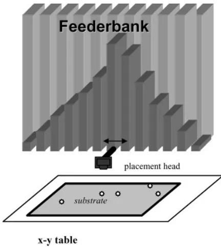
manufacturing [2, 11, 18]. PCBs are made up of an assort-ment of components—capacitors, resistors, etc.—that are mounted onto asubstrate. One method for doing so is with a through-hole pick-and-place machine that automatically selects and inserts the components, which are stored in a feederbank—a linear array of sleeves used to store the vari-ous components. Each sleeve contains components of a single type. A numerically-controlled conveyance requires tj sec-onds to move the retrieval head to sleevej, pick a component, return to the home position, and insert the component. [The board is simultaneously repositioned and thus the position on the board does not impact the production time.] It is easy to show (e.g. [19]) that, given a demand for a set of components of varying types, the retrieval time is minimized by sorting the component types according to decreasing frequency of use and then assigning them to sleeves of increasing dis-tance in the pick-and-place machine. Figure 1 shows this “pipe-organ” configuration.
Now consider the short-term problem of assembling a col-lection of different board types, in which a setup costσ is incurred whenever the machine is reconfigured, i.e. compo-nents are reassigned to new sleeves, to recognize the upcom-ing boards’ new characteristics. Because a “full tear-down” in which all components are removed and then restocked is typically used, so as to avoid error, this process is time-consuming and should therefore be taken into account in the planning process. Specifically, the problem requires the integration of clustering decisions (which boards to group together, when similar enough to permit a common set-up across them) and configuration decisions (how to assign components to sleeves). This problem,integrated clustering and machine setup(ICMS), addresses the problem of deter-mining the optimal trade-off between set-up and processing costs [21–23]. Although formulations other than set parti-tioning can be used to model this problem, the linearization of the objective function and the resulting weakness of the linear programming relaxation greatly restricts the size of instances that can be solved. We were able to achieve signif-icant improvements by instead formulating this problem as a set partitioning problem and then solving the pricing problem via RCP. We use this application to demonstrate our proposed approach.
The following notation is used:
• Kis the set ofjobs, i.e. distinct board types.
• Nis the number of distinct component types (and thus the number of sleeves in the pick-and-place machine). • qikis the demand for components of typeito satisfy
the production of boards of job typek.
• tj is the time to retrieve a component from sleevej. • fc∗(k) is the time to produce all boards of type k
[image:3.612.327.543.86.328.2]according to the pipe-organ setup which is optimal for the clusterC collectively; note that this setup is
Figure 1. A pick-and-place machine showing an optimal pipe-organ setup.
not necessarily the optimal setup for any individual boardkwithinC.
Given this notation, the objective coefficient for any cluster
C⊆Kis
σ+
k∈C
fC∗(k). (6)
the reduced cost is
σ +
k∈C
fC∗(k)−πk), (7)
and the pricing problem is therefore ICMS-PP
minσ+
k∈C
fC∗(k)−πk) (8)
st
C⊆K. (9)
3. THERANK-CLUSTER-AND-PRUNE ALGORITHM
3.1. Motivation
The motivation for a search-based approach to solving the set partitioning pricing problem stems from the fact that the cost of a cluster is often determined by a nonlinear function. Furthermore, there may be complex rules determining which clusters are feasible. The challenges of trying to address these in a MP approach are the very reason for using a set parti-tioning formulation in the first place, and these issues are thus also naturally problematic in the pricing problem.
Consider ICMS, for example. In this case, all nonempty subsets of K are valid clusters, but the objective function is nonlinear as it relies on the sorting of the components. Although this can be formulated as a MP, in our experi-ence the performance of such an approach is far too slow, especially when considering that this MP must be solved at each iteration of each node of the branch-and-bound tree. We demonstrate this with the following formulation, which is a MP-based approach to the pricing problem.
Recall that the purpose of the pricing problem is to identify a variable (i.e. the cluster or, in this case, the set of jobs) with negative reduced cost. In addition to the input data described earlier, we define three sets of binary variables.xk = 1 if board typekis included in the new cluster;yij =1 if com-ponenti is assigned to sleeve j when processing this new cluster; andwij k=1 if componentiis retrieved from sleeve jto meet the demand of boardkwhen processing this cluster.
The pricing problem can then be formulated as
minσ+
k∈K
N
i=1
N
j=1
qiktjwij k
−(πkxk)
(10)
st
i=1..N
yij =1 ∀j (11)
j=1..N
yij =1 ∀i (12)
j=1..N
wij k=xk ∀k,i (13)
wij k ≤yij ∀i,j,k (14)
xk,yij,wij k ∈ {0, 1} ∀i,j,k (15)
We denote the optimal objective value of the pricing prob-lem (independent of how it is found) by z∗(K). [TheK is included to indicate that this is optimal relative to the given set of objectsK—this will be relevant in the general state-ment of the algorithm, when the pricing problem is solved over varying sets of objects.]
At its core, this pricing problem must make two sets of decisions—which boards to include in the new cluster, and how to configure the pick-and-place machine for this cluster. Both of these can be formulated easily. Constraints (11) and (12) form anassignment problem, placing exactly one com-ponent in each sleeve. The binary variable restrictions onx
in (15) determine the make-up of the cluster. The remainder of the model is used to linearize the cost function, and this is the source of its complexity. Constraints (13) state that each component must be retrieved for a given board if and only if that board is included in the cluster. Constraints (14) state that a component cannot be retrieved from a sleeve unless it is assigned to that sleeve.
This formulation succeeds in linearizing the objective function, but fails to achieve tractability for all but the most trivial of problem instances. It suffers from two primary flaws. First, it is very large—on the order ofN2∗ |K|constraints and a comparable number of integer variables. For a problem with 24 board types and 100 component types, this is more than 240,000 constraints.
Second, and perhaps more problematic, is the weakness of the LP relaxation. Even for small problem instances, this model is slow to converge, because the model is able to “cheat” and only use the least expensive sleeves by selecting fractions of boards for the solution. Consider the following analogy. A child is told that he must eat all his dinner— chicken and peas (which he hates)—to have dessert. He proposes to eat half of his dinner in return for half of his dessert. His foolish mother agrees, only to discover the child eating all of the chicken but none of the peas. Similarly, in the model, if we only assign a fractional value toxkthen we only need fractional values for the retrieval variableswij k, which in turn enables the less expensive sleeves to be “shared” by multiple components in fractional amounts. In other words, we can gain the benefit of a fractional value of boardk’s dual while paying less than the equivalent fractional value of its processing cost.
The formulation can be strengthened through the use of cuts, but this further increases the constraint set. Certainly alternative formulations exist as well, but it would appear that any tractable formulation would require the use of deci-sion variablesxto select the boards; in testing many different formulations, we found that it was quite common for the branch-and-bound solver to branch on the majority of the
3.2. Algorithm
In this section, we first derive RCP in the context of ICMS, then generalize it and describe a class of set partitioning problems for which it is applicable.
3.2.1. Rank-Cluster-and-Prune for ICMS
The purpose of theRank-Cluster-and-Prunealgorithm is to take a set of board types (jobs) and their corresponding dual values, and generate a subset of these jobs with nega-tive reduced cost. The RCP algorithm has three steps. First, rank the board types by decreasing likelihood for inclusion in the new column. Second, construct a tree that explicitly constructs and computes the cost of possible clusters (i.e. sets of board types), at each depthdof the tree, branching on whether or not to include thedth-ranked board type. Third,
prunethe tree whenever possible to avoid full enumeration. This approach exploits three important characteristics of the problem to achieve tractability. First, it is trivial to com-pute the cost of a cluster. Second, the cost of a cluster always increases when another board type is added to it. Third, the only negative contribution to the reduced cost function is the duals associated with the board types in the cluster.
Rank. Consider the impact on reduced cost of adding board typekto an existing clusterC. By the optimality off∗and the fact that it is non-decreasing in set inclusion,
i∈C
fC∗∪{k}(i)−πi
+f∪{∗k}(k)−πk
≥
i∈C
fC∗(i)−πi
+fk∗(k)−πk
. (16)
Thus, addingkto the cluster must change the reduced cost by at least
pk≡fk∗(k)−πk, (17)
[image:5.612.323.555.84.253.2]which we define as thepotentialof boardk; in other words, this is a lower bound on the impact. We suggest that, in general, adding a board with more negative potential to an existing cluster is more likely to lead towards reduction in reduced cost. Note that for a board to have very negative potential, its minimum processing costfk∗(k)must be low, its dualπkmust be high, or both. A low processing cost might suggest a small number of components to be retrieved, in which case the board type would have limited impact upon the processing cost when being added to an existing clus-ter. Conversely, a high dual suggests that the board type is having negative impact on the ability of RM to find good solutions (i.e. this board does not fit well with other boards to form a logical cluster)—thus, new columns containing this
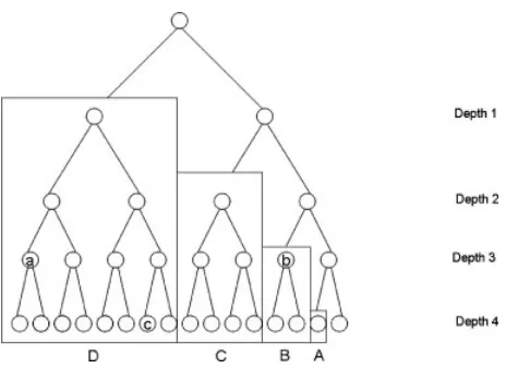
Figure 2. A sample RCP tree for an instance with four board types.
board type are desirable; on the other hand, if the board type is incompatible with other board types, then the subsequent additions of other boards to the cluster would quickly show an increase in overall cost and lead to easy pruning. Thus, we rank boards in increasing order of potential (i.e. beginning with the most negative).
Cluster. Given a ranked set of boards, we then construct a tree in which the root is the null set and has valueσ. We branch on this root node, creating two children—the left one, in which we add the highest-ranked board, which we will denote as board type 1, and the right one, which is a copy of its parent node (i.e. board type 1 is rejected and will not be reevaluated in any offspring of this node). The value of each of these nodes is determined by computing the reduced cost of the corresponding cluster. For each of these two nodes, we then branch, deciding whether or not to add the second ranked board, etc. For example, nodeain Fig. 2 corresponds to the cluster of boards ranked first, second, and third according to their potentials; its value is
σ+f{1,2,3}∗ (1)+f{1,2,3}∗ (2)+f{1,2,3}∗ (3)−π1−π2−π3. (18)
Nodebcorresponds to board 3, with cost
σ +f{3}∗ (3)−π3 (19)
and nodeccorresponds to boards 1 and 4, with cost
σ+f{1,4}∗ (1)+f{1,4}∗ (4)−π1−π4. (20)
Prune. If we fully construct the tree, at depth|K|we will have 2|K|nodes. Pruning is thus essential for tractability. We do so by again exploiting the notion of board potentials.
is added (becausef is non-decreasing in set inclusion) and thus we can preprocess out any such board.
Second, we consider the extension of this idea to cumula-tive potentials. Suppose we are at a node in the tree of depth
d −1. That is, our next decision at this node is whether or not to include the board ranked dth. Suppose also that the current node has nonnegative valueα. All remaining board types have negative potential (or else they would have been removed in preprocessing). If the sum of these potentials is not more negative than(−α), however, then the current node will never yield a negative reduced cost column and can be pruned (again, becausefis non-decreasing in set inclusion). We formally define thecumulative potential at depthdas
cpd ≡
|K|
i=d
fi∗(i)−πi
. (21)
Note that this potential depends only on the depth of the tree and not on the cluster itself.
Finally, we observe that even the cumulative potentials can be strengthened, because their computation is premised upon the notion that we can gain the value of all the outstanding boards’ duals but in turn only pay their individually-optimal processing costs. For example, if we are going to add to our cluster both boardsaandb, then at a minimum our processing cost would increase by
f{∗a,b}(a)+f{∗a,b}(b) (22)
rather than
f{∗a}(a)+f{∗b}(b), (23)
as is computed in the cumulative potentials.
It is not correct, however, to revise the potentials by replacing
|K|
i=d
fi∗(i)−πi
(24)
with
|K|
i=d
f{∗d,d+1,d+2,...|K|}(i)−πi
(25)
because we might be able to better improve our reduced cost by adding only some of the remaining outstanding board types. Rather, the lower bound should be stated asz∗ ({d,d +1,d +2,. . .|K|})−σ. In other words, this is the optimal reduced cost (minus the constant setup costσ) found when only considering boards of depthdor greater. That is to say, we can compute improved potentials by solving the pricing problem recursively, beginning with the lowest depth and moving upward, considering progressively larger subsets
ofK, with each solution providing bounding information for the higher iterations. We denote this tightened bound byβd. This is demonstrated in the formal statement of the algorithm in the following section.
3.2.2. RCP Algorithm
We use two data structures in solving RCP. We first define anodeto be a triplet comprised of a cluster, a value, and a tree depth. We then consider apending list, which is a linked list of nodes still to be examined.
Step 1:DefineK= {k ∈K : pk <0}. That is,Kis the subset of jobs that have negative individual potential and are therefore worth including in the search.
Step 2: Rank and re-index the elements ofKsuch that
p1 ≤ p2 ≤ · · · ≤p|K|. This is the order in which they will be evaluated in the tree, from most negative potential to least negative potential.
Step 3:Setβ(|K|)=p|K|. The cumulative potential at the lowest depth of the tree is simply the potential of the final board to be considered.
Step 4:Ifβ|K|+σ < 0, add the column corresponding to cluster{K}to RM. In other words, if we identify a clus-ter with negative reduced cost while we are constructing the potentials, then we can immediately add that cluster to the restricted master.
Step 5:For each depthd in decreasing order of potential (i.e.d = |K| −1,|K| −2,. . .1), compute the cummulative potentialβdaccording to the following steps. Note that these steps actually findz∗({d,d+1,d+2,. . .,|K|}), the optimal solution to the pricing problem relative to the restricted set of boards rankeddand higher.
Step 5a:Set thepending listto empty.
Step 5b:Setβ(d)=β(d+1). This initializesβ(d)(the most negative reduced cost that can be achieved by consider-ing all boardsdand higher) with the upper bound provided by the known value ofβ(d+1), which was computed in the prior iteration.
Step 5c:Createnode({d},pd,d). This is the root of the tree, which automatically contains boardd (sinceβ(d+1)
considers all clusters of boards with depthd +1 or lower, excluding boardd). This node has a value ofpd, the potential associated with boarddalone, and a depth ofd.
Step 5d:Addnodetopending list, thereby initializing the tree.
Step 5e:Whilepending listis not empty, select an arbitrary node and do the following. [We let (C,value,node_depth) denote the characteristics of this node.]
Step 5e2:Ifvalue+σ < 0, then the current cluster has strictly negative reduced cost. Therefore, add cluster C to RM.
Step 5e3:Ifnode_depth= |K|, then we have reached the bottom of the tree – prunenodefrompending list.
Step 5e4: Else, if node_depth < |K|, then we still
have remaining boards to consider. Check whether value +βnode_depth+1≥βd. In other words, is the current value plus the potential of the board types remaining to be considered guaranteed to be no better than the current bound onβd? If so, prune node frompending list.
Step 5e5:Else, ifvalue+βnode_depth+1< βd, then the cur-rent cluster can potentially be improved. Thus, we need to evaluate the tree below it. We do so by branching according to the following two steps.
Step 5e5a: Setnode_depth=node_depth+1, i.e. drop down one level in the tree. This is equivalent to the right-branch in the tree, i.e. we reject the next candidate board from the cluster.
Step 5e5b:Create anew_nodetoincludethe next candi-date board in the cluster—this is equivalante to the left-branch in the tree. Set the cluster ofnew_node to{C∪node_depth}, the value ofnew_nodeto the optimal processing cost of this new cluster minus the sum of its duals, and the depth of new_nodetonode_depth. Addnew_nodetopending_list.
EXAMPLE 1: To clarify this, we refer the reader again to Fig. 2. In this tree, there are four depth levels. This means that there are four boardskin the data set for which
fk∗(k)−πk. (26)
We label these boardsA,B,C, and D, whereD has the most negative potential (and thus is evaluated at the top of the tree) and Ahas the least negative (but still strictly less than zero) potential and thus is evaluated at the bottom of the tree.
The first step is to compute the cumulative potential of boardA. This is simply the individual potential ofA,
β(A)=fA∗(A)−πA, (27)
which by supposition is strictly negative. We then compute
β(A)+σ. (28)
If this is strictly less than zero, then we add the column associated with the cluster{A}to the restricted master.
Next, we compute the cumulative potential of boardB— that is, the maximum value that can be gained by considering boards of depth three or lower. In other words, we want to find the minimum of the clusters{A},{A,B},{B}. To do so
we first check whetherfB∗(B)−πB+σ <0. If so, we add
the cluster{B}to the restricted master. Next, we compare
β(A)tofB∗(B)−πB. By our choice of ranking,β(A)will always be lower and thus we set β(B) = β(A). We then create the node associated with cluster{A,B}and compute
fA∗,B(A)+fA∗,B(−B)−πA−πA. If this is strictly less than β(B)then we updateβ(B)with this value. We also check to see if addingσto this yields a strictly negative cluster; if so, we add{A,B}to the restricted master.
In the third stage, we compute the cumulative potential of board C. In this case, suppose that when we evalu-ate the node associevalu-ated with cluster {C,B}, we find that
fC∗,B(C)+fC∗,B(B)−πC−πB+β(A)≥β(C), then we can prune—i.e. addingBtoCmakes us worse off than keeping
Calone.
Finally, we complete the algorithm by computing the potential for boardDand, in the process, effectively evaluat-ing the entire tree, takevaluat-ing advantage of the recently computed cumulative potentials to reduce branching.
3.2.3. Details and Observations
Generating Multiple Columns. Note that it is not necessary in a delayed column generation approach to find themost neg-ative reduced cost column when solving the pricing problem (this is an important factor in the tractability of approaches such as multilabel shortest paths (e.g. [5, 14])—we simply must find a column with reduced cost strictly less than zero in order for the column generation approach to converge. Thus, whenever we encounter a negative reduced cost column while constructing potentials, we can add this to RM. Furthermore, it is often beneficial to add multiple new columns to RM in a single iteration of the pricing problem. In our computational experiments, we often found very large numbers of negative reduced cost columns after examining only a fraction of the RCP tree.
Avoiding Repetition. In the act of constructing cumulative potentials, we are actually fully evaluating a portion of the original tree. Thus, this portion of the tree does not need to be reevaluated subsequently. In fact, if we compute the poten-tials of each depth from |K| all the way up to 1, then the algorithm is complete—the tree will have already been fully evaluated. For example, in Fig. 2, we first evaluate the node in blockAto findβ4, then blockBto findβ3, then blockC to findβ2, and finally blockDto findβ1. This fully exhausts the tree. Note that these blocks are not necessarily fully enumerated, as nodes may be pruned within them by lever-aging the potentials already computed for lower depths of the tree.
computationally to process it as a singly-linked list. By defin-ing each node in the tree to store its depth, its current cluster (which can be stored as a binary number), and its current value, we do neither need to keep pointers from child nodes to parent nodes, nor do we need to retain nodes after they have been evaluated and split. When we process a node, we first compute its value (i.e. the reduced cost of the corresponding cluster). If the node has (strictly) negative reduced cost, then we immediately return its cluster to RM. After computing the cost, we check to see if the node can be pruned. If not, we then make a copy of the node and, in this copy, increase the depth and add the next ranked board to the cluster (this corresponds to the left branch). We can insert this immediately after the current node in the linked list for a depth-first search, at the end of the list for a breadth-first search, or in the appropriate location for a best-bound search, as a function of its current reduced cost. In addition, we also keep the original node, but increment its depth, thereby converting the current node to the right branch (associated with rejecting the next ranked board type).
Termination Criteria. It is not necessary to fully evaluate the pending list except in the final instance, in which opti-mality is proven by the lack of any negative reduced cost columns. So long as at least one valid column has been found, the tree can be terminated at any time. It is trivial to set limits on run time, number of evaluated nodes, or number of generated columns, after which the algorithm should be terminated. In Section 4, we demonstrate the power of this fact.
Branching. Finally, although the focus of this article has been on the pricing problem, which is an integral part of solving the individual LPs in the branch-and-bound tree, we conclude with a brief note about branching strategies for RM. It is common when solving IP’s to branch on variable dichotomy—given a fractional value forx, setx =1 in one half of the tree andx=0 in the other. Such a strategy can be problematic in branch-and-price, because this new constraint is accompanied by a new dual value which only applies to a single solution to the subproblem. Thus, in set partitioning problems, it is common to insteadbranch on object pairs— in one half of the tree, objectsa andbmust be included in the same cluster and in the other half, they must not (see, for example, [26] and [27]). In our proposed approach, it is triv-ial to enforce this branching strategy and, in fact, this even improves performance as the depth of the RM branch-and-bound tree grows. For a node of the branch-and-branch-and-bound tree wherea andb must be together, then whenever we adda
to a cluster as we are solving the subproblem, we prune the portion of the RCP tree underneath it in whichbis rejected and vice versa; the opposite is true on a branch whereaand
bmust be separate.
3.2.4. RCP for General Set Partitioning Problems The RCP algorithm, as described in the preceding section, can easily be extended to problems other than ICMS. Only the following two conditions are needed:
• It must be possible to compute the cost functionf (g)
associated with clustergquickly. Note that this does not require linearity or even convexity off. In fact, we do not require thatf be a closed-form function. There must simply be an oracle that can quickly return
f (g)for any clusterg.
• f (g)must be less than or equal tof (g∪C)for all setsC(i.e. adding to a cluster cannot decrease its o cost).
Note that our initial statement of the algorithm (with respect to ICMS) assumes all clusters are valid clusters. This also need not be the case—so long as a cluster can easily be tested for feasibility, we simply add that step at each node (again, not that we do not require a MP approach to testing these feasibility—any oracle is acceptable).
In addition, the following characteristics (not present in ICMS) will improve the performance of the algorithm:
• Suppose that if the reduced cost of setgis less than the reduced cost ofg∪ {i}, then the reduced cost of gis less than the reduced cost ofg∪ {i} ∪Cfor any objectiand any setC. In other words, if adding an object to the setgincreases its reduced cost, then the reduced cost of any further expansion of the setgwill never have lower reduced cost either. Then whenever a child node has greater value than that of its parent, that branch of the tree can be pruned.
• Suppose that all constraints are “additive” – if setg
violates the constraint, then setg∪Cwill also violate the constraint for any setC. Such constraints include limits on the maximum number of elements in a set, their maximum weight, and so forth. In such a case, whenever a node is encountered that violates these constraints, then again the tree can be pruned from this node.
these problems challenging (see, for example [9]) is the col-lection of requirements as to what constitutes a valid district. For example, the neighborhoods in a district typically must be contiguous, cannot span natural boundaries such as rivers or major roadways, and must satisfy certain requirements of diversity. These requirements are often straightforward to test for—that is, given a set of neighborhoods, we can eas-ily determine whether it satisfies the requirements—and yet formulating these checks in a mathematical programming construct can be quite problematic. As such, RCP provides a natural alternative, because the feasibility test can be encoded as a “black box” rather than through linear constraints. Simi-lar problems exist in districting for electric power markets [6], police districting [12], and home health-care districting [7]. Finally, we note that certain special classes of vehicle rout-ing and crew schedulrout-ing problems may be ammenable to an RCP approach. For example, in a drayage operation where the dominant cost is a function of the customers served, rather than the distance traveled, RCP might be applicable. In this case, the challenge would be in determining the feasibility of a set of loads from a timing standpoint. This again is in some cases difficult to capture with a set of linear constraint but can naturally and quickly be solved via a “black box” feasibility checker.
4. COMPUTATIONAL RESULTS
Our computational experiments were conducted on a test bed of ICMS problem instances generated by Norman [24]. This data set (available at http://www-personal.umich.edu/∼amycohn/papers.html), from which we extracted 13 problem instances (referenced by their nam-ing from [24]), was designed to capture a variety of man-ufacturing characteristics and based on actual optimization problems on the shop floor. Recognizing that the key trade-off is between retrieval times and the machine setup time, we considered three different values of the setup timeσfor each instance (derived from the particular instances’ parameters to consider cases where there are large, medium, and small numbers of clusters in the optimal solution). Each RM was initialized with a set of columns containing one-, two-, and three-item clusters,|K|−1,|K|−2, and|K|−3 item clusters, and the exhaustive cluster.
We coded the branch-and-price algorithm in C++, using CPLEX 8.0 to solve the individual restricted master LPs. Branching was conducted using the strategy outlined in Section 3.2.3. For each individual LP, RCP (also implemented in C++) was used to generate the columns. We permitted up to 10,000 negative reduced cost columns to be added to RM at each iteration of the pricing problem. We terminated RCP if at least one negative reduced cost column had been found and more than 2,500,000 nodes in the RCP tree had
Table 1. Single instance.
Data set A4 Iteration Evaluated nodes Col’s
No. of boards 24 1 26178(0.16%) 10,000
No. of components 16 2 63, 382(0.38%) 10,000
σ 5000 3 87, 873(0.52%) 10,000
Max nodes per tree 16,777,216 4 107, 923(0.64%) 10,000
Total time 36 s 5 94, 037(0.56%) 10,000
6 96, 793(0.58%) 10,000 7 97, 714(0.58%) 10,000 8 153, 029(0.91%) 8,473
9 140, 314(0.84%) 137
10 179, 595(1.07%) 16
11 170, 043(1.01%) 0
been investigated or more than 10,000 negative reduced cost columns had been found.
We solved each of the problem instance to integer optimal-ity (with the exception of one instance, for which we were unable to solve the LP relaxation to provable optimality). There was very little branching, as is often seen in set par-titioning problems of this size. The instances often required fewer than 10 nodes to be solved in the branch-and-bound tree of the master problem and never required more than 50 nodes to be solved. In addition to noting the limited branch-ing in our problem instances, we also note that the overall performance issues associated with column generation and branch-and-price relative to the master problem are indepen-dent of the mechanism used to solve the pricing problems (other than, of course, the run time of the pricing problem iterations themselves). [See [28] and [30]) for further dis-cussion.] Therefore, the remainder of our discussion on the computational experiments focuses specifically on the per-formance of the pricing problems in solving the root node of the branch-and-bound tree.
We begin in Table 1 by providing detailed information about a single, illustrative example. This problem instance has 24 boards, 16 components, and a setup time ofσ =5000. It took 11 iterations of the resticted master (i.e. eleven calls to the pricing problem, via RCP) to solve the LP relaxation to provable optimality, with a total run time of 36 s. The first seven iterations of the pricing problem terminated according to the stopping criteria of having identified 10,000 negative reduced cost columns. The remaining columns terminated after the tree was exhausted. The final iteration did not yield any negative reduced cost columns and thus established opti-mality of the LP. Note that the number of nodes actually evaluated in the tree was rarely above 1% of the total possible size(224 =16, 777, 216). In other words, the vast majority of the tree was pruned without the associated clusters being explicitly evaluated.
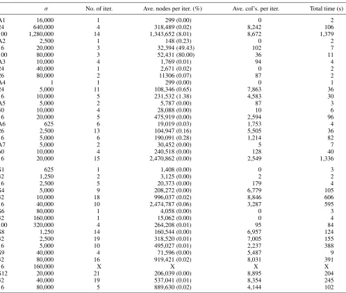
Table 2. Results.
σ No. of iter. Ave. nodes per iter. (%) Ave. col’s. per iter. Total time (s)
A1 16,000 1 299(0.00) 0 2
24 640,000 4 318,489(0.02) 8,242 106
100 1,280,000 14 1,343,652(8.01) 8,672 1,379
A2 2,500 1 148(0.23) 0 2
16 20,000 3 32,394(49.43) 102 7
100 80,000 3 52,431(80.00) 36 11
A3 10,000 4 1,769(0.01) 94 4
24 40,000 1 2,671(0.02) 0 2
26 80,000 2 11306(0.07) 87 2
A4 1 1 299(0.00) 0 1
24 5,000 11 108,346(0.65) 7,863 36
16 10,000 5 231,532(1.38) 4,583 30
A5 5,000 2 5,787(0.00) 87 3
40 10,000 4 28,088(0.00) 10 6
16 20,000 5 475,919(0.00) 2,594 96
A6 625 6 19,019(0.03) 1,753 4
26 2,500 13 104,947(0.16) 5,505 36
16 5,000 6 190,091(0.28) 1,214 82
A7 5,000 2 30,452(0.00) 5 7
60 10,000 4 240,518(0.00) 128 40
16 20,000 15 2,470,862(0.00) 2,549 1,336
S1 625 1 1,408(0.00) 0 3
32 1,250 2 3,125(0.00) 2 2
16 2,500 5 20,373(0.00) 179 4
S4 5,000 9 208,272(0.00) 6,779 105
32 10,000 18 996,037(0.02) 8,846 606
16 40,000 10 2,474,787(0.06) 3,287 595
S6 80,000 1 4,058(0.00) 0 3
32 160,000 1 15,062(0.00) 0 4
100 320,000 4 264,208(0.01) 95 84
S8 1,250 14 160,544(0.00) 6,957 124
32 2,500 19 318,520(0.01) 7,005 155
16 5,000 10 495,027(0.01) 2,237 388
S9 40,000 4 71,596(0.00) 5,487 9
32 80,000 16 919,421(0.02) 8,031 391
16 160,000 X X X X
S12 20,000 21 206,039(0.00) 8,895 204
32 40,000 19 537,041(0.01) 8,354 245
16 80,000 5 889,630(0.02) 4,144 102
indicates that the instance could not be solved to completion in under an hour; there is one such instance. The first column of these tables lists the data set (labeled by the numbering of [24]), number of boards, and number of components. There are three instances per data set—the second column gives the three values ofσ. The third column gives the number of calls to the pricing problem. The fourth column gives the aver-age number of nodes evaluated per iteration as well as the percentage of nodes relative to a fully-enumerated tree. The fifth column gives the average number of columns gener-ated per iteration (excluding the final call, which establishes optimality). The sixth column gives the total run time. All iter-ations solved in under an hour (in most cases, substantially so) except one. Data set S9, with a value ofσ =160,000, did not terminate within an hour of run time. We believe that is
a function of degeneracy, which is quite common in set par-titioning problems. In particular, when the setup cost is very large and thus the number of clusters included in the optimal solution is very small, the vast majority of basic variables are degenerate, which can lead to excessive pivoting. In contrast, the most successful alternatives that we have seen in the liter-ature, using traditional MIP-based approaches, cannot solve problems larger than 8–12 boards types [21].
5. CONCLUSIONS AND FUTURE RESEARCH
approach, RCP, may be a viable alternative. For example, this approach enables the solving of instances of ICMS that could not be solved prior to this approach. In RCP we leverage the fact that the cost function is straightforward to compute off-line but difficult to off-linearize in an MP formulation, and we reduce the number of clusters that are explicitly considered in this enumerative approach by pruning the tree through the use ofpotentials. Recursively computing progressively tighter bounds on the potentials by solving increasingly large subsets of the pricing problem greatly improves the quality of these potentials and thus the performance of the algorithm. This is demonstrated by our computational experiments, in which typically less than one percent of the tree needed to be explored to find provably optimal solutions.
Areas for future research include developing additional methods for pruning the RCP tree and considering the impact of alternative ranking strategies on performance.
ACKNOWLEDGMENTS
The authors wish to acknowledge the computational efforts of Reid Tatoris.
REFERENCES
[1] E. Balas and M. Padberg, Set partitioning: A survey, SIAM Rev 18 (1976), 710–760.
[2] M.O. Ball and M.J. Magazine, Sequencing of insertions in printed circuit board assembly, Oper Res 36 (1988), 192–201. [3] C. Barnhart, E. Johnson, G. Nemhauser, M. Savelsbergh, and P. Vance, Branch-and-price: Column generation for solving huge integer programs, Oper Res 46 (1998), 316–329. [4] C. Barnhart, C. Hane, and P. Vance, Using
branch-and-price-and-cut to solve origin-destination integer multicommodity flow problems, Oper Res 48 (2000), 318–326.
[5] C. Barnhart, A. Cohn, E. Johnson, D. Klabjan, G. Nemhauser, and P. Vance, Handbook of transportation science, 2nd ed., Kluwer’s International Series, 2003.
[6] P. Bergey, C. Ragsdale, and M. Hoskote, A decision support system for the electrical power redistricting problem, Decision Support Syst 36 (2003), 1–17.
[7] M. Blais, S. Lapierre, and G. Laporte, Solving a home-care districting problem in an urban setting, J Oper Res Soc 54 (2003), 1141–1147.
[8] B. Bozkaya, E. Erkut, and G. Laporte, A tabu search heuristic and adaptive memory procedure for political districting, Eur J Oper Res 144 (2003), 12–26.
[9] F. Caro, T. Shirabe, M. Guignard, and A. Weintraub, School redistricting: Embedding GIS tools with integer programming, J Oper Res Soc 55 (2004), 836–849.
[10] D. Cattrysse, M. Salomon, R. Kuik, and L. Van Wassenhove, A dual ascent and column generation heuristic for the discrete lot-sizing and scheduling problem with setup times, Management Sci 39 (1993), 477–486.
[11] Y. Crama, J. van de Klundert, and F.C.R. Spieksma, Production planning problems in printed circuit board assembly, GEMME 9925, University of Liege, Liege, Belgium, 1999.
[12] S. D’Amico, S. Wang, R. Batta, and C. Rump, A simulated annealing approach to police district design, Comput Oper Res 29 (2002), 667–684.
[13] G. Dantzig and P. Wolfe, The decomposition principle for linear programs, Oper Res 8 (1960), 101–111.
[14] G. Desaulniers, J. Desrosiers, I. Ioachim, M. Solomon, F. Soumis, and D. Villeneuve, A unified framework for deter-ministic time constrained vehicle routing and crew scheduling problems, Fleet Management and Logistics, T. Crainic and G. Laporte (Editors), Kluwer, Boston, 1998, pp. 57–94. [15] J. Desrosiers, N. Mladenovic, and D. Villeneuve, Design of
balanced MBA student teams, J Oper Res Soc 56 (2005), 60–66.
[16] T. Fahle, U. Junker, S. Karisch, N. Kohl, M. Sellmann, and B. Vaaben, Constraint programming based column generation for crew assignment, J Heuristics 8 (2002), 59–81.
[17] P. Gilmore and R. Gomory, A linear programming approach to the cutting stock problem, Oper Res 11 (1963), 863–888. [18] H.O. Günther, M. Grunow, and C. Schorling, Workload
plan-ning in small lot printed circuit board assembly, OR Spektrum 19 (1997), 147–157.
[19] G. Hardy, J. Littlewood, and G. Polya, Inequalities, 2nd ed., Oxford University Press, 1952.
[20] S. Hess and J. Weaver, Nonpartisan political redistricting by computer, Oper Res 13 (1965), 998–1006.
[21] M.J. Magazine and G.G. Polak, Job release policy and printed circuit board assembly, IIE Trans 35 (2003), 379–387. [22] M.J. Magazine and G.G. Polak, Optimal machine setup and
product clustering for printed circuit board manufacturing, Raj Soin College of Business Working Paper 02-006, Wright State University, Dayton, Ohio.
[23] M.J. Magazine, G.G. Polak, and D. Sharma, A multi-exchange neighborhood search heuristic for an integrated clustering and machine setup model for PCB manufacturing, J Electron Manuf 11 (2002), 107–119.
[24] S.K. Norman, Heuristic approaches to batching jobs in printed circuit board assembly, Ph.D. dissertation, QAOM Depart-ment, University of Cincinnati, 2001.
[25] C.C. Ribeiro, M. Minoux, and M. Penne, An optimal column-generation-with-ranking algorithm for very large scale set partitioning problems in traffic assignment, Eur J Oper Res 41 (1989), 232–239.
[26] D. Ryan, The solution of massive generalized set partition-ing problems in aircrew rosterpartition-ing, J Oper Res Soc 43 (1992), 459–467.
[27] D. Ryan and B. Foster, An integer programming approach to scheduling, Comput Sched Public Transport, A. Wren (Editor), North-Holland, Amsterdam, 1981, pp. 269–280.
[28] M. Savelsbergh, A branch-and-price algorithm for the generalized assignment problem, Oper Res 45 (1997), 831–841.
[29] C. Tang and E. Denardo, Models arising from a flexible manufacturing machine. II: Minimization of the number of switching instants, Oper Res 36 (1988), 778–784.
[30] F. Vanderbeck, On dantzig-wolfe decomposition in integer programming and ways to perform branching in a branch-and-price algorithm, Oper Res 48 (2000), 111–128.