Micro Based Estimates of Demand Functions for Local School Expenditures

Center for Research on Economic and Social Theory

Research Seminar in Quantitative Economics

Discussion Paper

DEPARTMENT OF ECONOMICS

University of Michigan

Micro-Based Estimates of Demand Functions for Local School Expenditures

Theodore C. Bergstrom

Daniel L. Rubinfeld Perry Shapiro

C-28

Dept. of Economics, the University of Michigan

October 1980

I. Introduction

Individual preferences are as central to modern public goods analysis as

they are to the study of markets for private goods. The well-known Samuelson conditions for efficient provision of public goods involv the sun of indivi-duals' marginal rates of substitution between public and private goods. Economic

theories of the behavior of democratic governments have it that the supply of public goods by a community is determined by the pattern of preferences in the-electorate.1- Thus, whether we wish to investigate the efficiency of government institutions or to forecast the effects of anticipated changes in economic and demographic variables on public expenditure, we could like to be able to relate the indifference maps of individuals to observable characteristics of these individuals and their environments.

A standard result in the theory of demand for private goods is that (subject to certain regularity conditions) knowing a consumer's demand function is

equivalent to knowing its indifference map. Thus if one observes what a rational consumer would choose in many different price--income situations, one can estimate a demand function. Furthermore, the demand function can be made to depend on demander's observable characteristics, such as age, race, or sex. The demand functions thus estimated can, in turn be "integrated back" to find indifference maps for consumers with each possible list of characteristics. Our objective in

this paper Is to accomplish a similar program for a particular publically provided 2/

good, namely local elementary and secondary

education.-Estimating demand functions for public goods is in certain respects less

straightforward than doing so f or private goods. One can observe a consumer's

income and other characteristics as well as the "tax price" that it pays per unit

of public goods and the amounts of public goods provided in its commnu:ity. But one can not be certain that the consumer gets the amount of public goods that it

would like to have, given the tax price that it pays, The quantity of public

-2-be the unanimous choice of all citizens,

In democracies, the fundamental behavioral indicator of preferences for public goods is voting behavior. Of course with the Australian ballot, one

can not observe how any particular individual votes. Rather, one observes the "aggregate" outcomes of elections and referenda, A possible method of estimat-ing demands for public goods is to relate aggregate outcomes of elections in

different places to indicators of the economic and demographic composition of their populations. Several studies of this type are discussed in review articles by Denzau (1975), Deacon (1977), and Inman (1979). Deacon classifies these

studies into two groups -- those based on "majority rule--median voter models"

and those based on voting behavior. The former group, following a line of research begun by Barr and Davis (1966), attempt to infer individual demand functions from cross-sectional studies in which actual public expenditures by local governments are regressed on indicators of the economic and social. composi-tion of the jurisdiccomposi-tion's populacomposi-tion, In order to draw such inferences, one

needs a "political" theory that relates a jurisdiction's expenditures to the

profile of preferences of its population. The theory most often used is the "median voter theory" developed by Bowen (1943). Bergstrom and Goodman (1973) give this theory specific empirical content by showing that, subject to certain

strong assumptions, majority rule implies that one can treat an observation of

expenditure levels in a given jurisdiction as a point on the "demand curve" of a citizen of that community with median income for the community. This procedure has the advantage of presenting the researcher with a very large cross-sectional data base at very low cost in data collection. There are, of course, thousands

of local government units in the country, varying widely in the characteristics

of their populations and in their expenditure levels, Furthermore the U.S.

censuses of population and of governments offer quite detailed information about

-3-has the disadvantage that the reliability of its estimates of demand functions depends at least in part on the degree to which the political process

is-approximated by the median voter model. Reliability also depends on certain-regularities in the structure of demand in the. community, as remarked in Bergstrom and Goodman (1973).

The "voting behavior" studies typically estimate demand functions by relat-ing the proportion of favorable votes on a public goods referendum in a precinct

4/

to indicators of the economic and demographic make-up of the precinct.- Where each precinct is a single observation and where all precincts are voting on the same issue, one typically must settle for a fairly small number of observations. In general, data of this type are much sparser and more difficult to acquire than the data needed for the "median voter" estimates. Furthermore, as we shall discuss later, data on voting in a single election are not, in general, adequate to fully identify a demand function although they can supply useful qualitative

information about the determinants of demand.

Both "aggregate" methods of estimation depend on subtle inferences that allow many possibilities for statistical misspecification. With these methods

it is virtually impossible to distinguish the effects of individual characteristics,

(e.g., income or race) from those of "neighborhood characteristics (e.g., community

income or racial composition). Another potential source of error, as pointed out by Goldstein and Pauly (1980), is a "Tiebout bias" which could result from people sorting themselves into communities in response to similarities in desired levels of public goods. Since there is cause for reservations about the reliability of demand estimates founded on aggregate data, it is of cons. >rable interest to

discover whether the results of such studies are consistent with microeconomic

-4-It. A Nethod of Estimating Continuous Demand Equations from Qualitative Survey Responses.

So long as there is a secret ballot, it would seem that the only way to

find out whether an individual is satisfied with his current level of public

goods consumption is to ask him. Surveys of voter sentiment and intentions,

such as the Gallup poll, are common, Surveys that systematically relate a

voter's expressed preference to standard economic variables are rare. Interest-ing examples of the use of survey data to relate votInterest-ing behavior to economic variables are studies by Rubinfeld (1977), Fischel (1979), and Citrin (1979).

To date, however, we are aware of no estimates of demand functions for a public 5/

good based on survey data.-

-In this paper we develop a method for estimating demand functions for public goods from survey data and proceed to estimate these functions. The

data used in the paper were obtained from a survey of 2001 individuals in

Michigan, selected randomly, immediately after the November 1978 election.

Detailed discussions of the construction of the survey are available in Courant,

Granlieh and Rubinfeld (1979, 1980).- Although the Courant, Gramilich, Rubinf eld

survey inquired about demands for several types of public expenditure we confine our attention in this paper to school expenditures.

The interviewers asked each respondent:

"Do you think the state and local governments should be spending more, spending less, or about the same amount

on the local public school system as they are spending now?"

If the response to this question was "more," it was followed by a second question: "If your taxes had to be rais ed to pay f or the

addi-tional expenditures on local public schools would you still favor an increase in expenditur e in this

area?"-If the response was "e" to this second question, the respondent was recorded as favoring 'more" expenditure on schools. If the response was "no" to this question,

-5-Thus for each respondent an answer of "more," "less" or "the same" was recorded. Respondents were also asked to state their incomes, their annual property tax

bills, whether they are owners or renters, their race, age, number of children

and several other personal characteristics. Asking a simple qualitative

ques-tion about the direcques-tion of the respondent's preferred amount of public

expenditure from the status quo, rather than asking him to specify more exactly how much he would like, reduces the burden on the respondent's imagination. On the other hand, the economist using such data must perform theoretical and statistical machinations which would be unnecessary if he observed actual quantities demanded instead of "mere" qualitative information.

To characterize the problem quite generally, let the vector xi be a list of observable variables describing an individual and his environment. Let q. be the amount of a public good that the individual would most like his community to supply, given that he would have to pay his current share of the tax cost

of any hypothetical level of- expenditures. Let ai be the amount act'>illy supplied by his community. Suppose that the individual's most preferred amount of public good is

(1) q. = D(xi) + c.

where E. is the ith realization of some random variable e and where D(x.) is a "demand function".

The set-up here will be familiar to those acquainted with the ec .metric 7/

and biostatistical literature on qualitative choice models.- If we hypothesized

that individual i answers "more" whenever q. > a., "less" whenever q. < a. and

-6-of the event q = ai is zero for each i. This formulation would therefore be consistent with the data only if almost none of the respondents claimed to be satisfied with current levels of provision of public goods. In fact, it turns out that 58% of the homeowners in the sample said that they wanted "about the same" as the current level of expenditures in their districts,

while 25% claimed to want "more" and 17% claimed to want "less".

We therefore chose to recast the model to assume that voters whose

preferred level of public goods supply differed from the actual level by less than some threshhold proportion would say "about the same." Thus we assume that for some parameter, 6 > 1, the respondent claims to want "more" if

> 6a "less" if q< ai and "about the same" if ai q 8a .

6 6aq

Taking logs and using equation (1), we see that the respondent is assumed to answer "more" "less" or "about the same" respectively, if:

(2)

Inc.

Ina.

(3) Ins > lnD(x.) + 1n6 - Ina.

i i2 *, 2

(4) lnD(x ) - 1n6 - lna. < ins < lnD(x.) + lnS - Ina.

i .1i= i= = .

9/ For purposes of estimation, we assume that ins has a logistic distribution- with

zero mean and an unknown standard error, a. Then Inc has a logistic distribution with zero mean and unit variance. Let F(-) denote the cumulative distribution of the logistic with zero mean and unit variance. Suppose that lnD(x i,... ,xik)

k

S + $.X... From equations (2) , (3) and (4) , it then follows that the

likeli-hood functions for the responses "more" and "less" are r espectively:

(5) F( -0 ( ) x. . - - Ind - - la.)

and -

_2.

(6) 1- F(# + k x. +inS - .. lna.)

a . 3 i

while the likelihood of the answer "about the same" is one minus the sum of (5)

-7-Using a standard computer program for estimation of an ordered logit model,

8 1

we obtain estimates of the coefficients, (SJ

),

aj

and a in equations (5) and (6). From these estimates we can obtain estimates of 8. by simple division. The logit routine also yields estimates of the "intercept terms" So+ 1 lnd and o - 1 lnd. From these estimates and our

estimates of 1, we can calculate an estimate of Ind.

From expressions (5) and (6) it is apparent that in order to estimate the

10/

parameter 1, we must observe variation in the a i's.-- For cxample, in Rubin-Q

feld's 1977 study, all of the observations were of people living in a single community. Thus Rubinfeld was able to estimate the ratio of the price elasticity to the income elasticity of demand, but he was not (as he remarked) able to

estimate these elasticities themselves. The same difficulty precludes estimation of a demand function from observations of precinct returns in an expenditure referendum in a single jurisdiction.

Even with data such as ours, where we observe expenditure levels in several places, the precision of our estimates of the parameters is seriously limited by the relatively small amount of variation in expenditure levels. Thus, although we sample nearly one thousand consumers, they live in only about one hundred different school districts. Our sample, therefore, has much more variability in the x,., variables than in the ai's. Consequently we find that the standard errors of the estimates of 1 are about five times as large as those for the coefficients,

S 11/

i, on income and

price.---a

III, Measuring Pr ic e and Quantity

The demand eqiuation that we estimate has the form: k

-8-where E is the respondent's desired level of per student school expenditures in

his school district, t is the estimated tax cost to the respondent of an additional dollar of expenditures per pupil in his district, Y is his income after local

taxes and the x 's are a number of other descriptive variables.

We measure quantity by expenditure rather than physical units, because the production of education requires many different inputs and there is no really

satisfactory physical measure of output. This procedure would be entirely appropriate if all observed school distr J.cts faced the same input prices and had the same "production function" for education. In this case, expenditure provides a scalar measure, which is monotonically related to the quality of

local education. If, on the other hand, there were variations in factor costs from place to place, expenditure would not be a good measure of quantity.

Further-more, the "price" and income variables used should be adjusted to account for any local variations in the costs of private goods as well as the cost of

educational inputs.

Suppose that the price level for educational inputs in the respondent's

district is pe and the price level for all other goods is p0. Then equation

(1) would be more properly rewritten as

tpE k

(2) in- -$ + ln- +a 2 n-+ S. x+ .

p

p

Po

where expenditures on education and on other goods are adjusted by the appro-priate local price indices so as to measure quantities and where the price, t -,

p₀

represents the quantity of other goods that the respondent must give up in order

to acquir e an add

itional

equa-tion (2) is equivalent to:

(3)InE= 8+ 6int+ 8 + 1 +3 )n p -- (Si+ 8)A"o + 6 x+ E

.9.

Therefore, if we estimate (1) without including the variables pV and p , the estimates are subject to bias because of omitted variables. While we can not obtain good direct measures of pE and p0, we have access to some variables

which are closely related. These include the average teachers' salary and an index of average wages in the private sector in the county where the respondent

12

/

lives.-- It is hoped that use of these variables will largely eliminate bias from the omission of price indices.

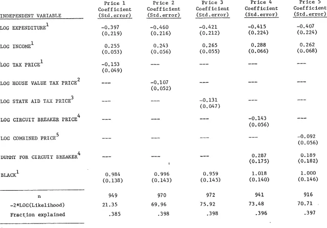
Conceptually, the notion of "tax price" that we want is the marginal cost to an individual of increasing the amount of expenditures per student in the

131

school district where he resides by one dollar.-- Essentially all locally raised school funding is obtained from the property tax. Therefore, if marginal increments to local expenditures came entirely from local sources, the tax price paid by an individual would be equal to the number of students in the local school district times the ratio of the assessed value of his property to the total assessed value in the district where he lives, The survey allowed us to make two independent estimates of this' number. Respondents were asked to

estimate the amount of property taxes that they paid per year. They were also asked to estimate the market values of their houses. Using published data on millage rates, assessment to market value ratios and school enrollment, we constructed a tax price based on each of these estimates. These two estimates frequently differ quite substantially. Demand functions estimated by using each of these concepts of tax price are reported in the first two columns of Table 4. Fortunately, the estimates found in these different ways are very similar. We chose to confine our further analysis to the case of estimates based on the

-respondent's notion of his tax bill on the grounds that the f its obtained with

-10-Further complications are introduced by two important distributional programs operated by the state of Michigan. One of these is the state aid-to-education program. The other is the so-called "circuit breaker" property tax relief

program which allows taxpayers a credit against their state income taxes, the size of which depends on their local property tax bills.- 4 The current Michigan state aid formula is not lump sum, but alters marginal costs to local taxpayers. Likewise the circuit breaker programs reduces the net cost to certain taxpayers

of a marginal expenditure on local education. Using the explicit formulae for each plan and the data we have about each individual and his district, we are able to compute the marginal tax prices that apply to each individual when these programs are taken into account. The coefficients are not much changed by

inclusion of these effects as we will show in Table 3 below. Perhaps one reason why the coefficients are not substantially affected is that both programs are

quite new and probably are not well understood by the electorate. Until 1973-74,

Michigan state aid was essentially lump sum in character. Since then, there has been a significant matching component for many districts, but the operating formula has been changed quite drastically in each succeeding year. (See Brazer and Anderson (1976)). The circuit breaker was introduced in 1974, and its

implications for the marginal cost of local public goods to taxpayers do not seem to be widely understood.

IV. Results and Interpretation

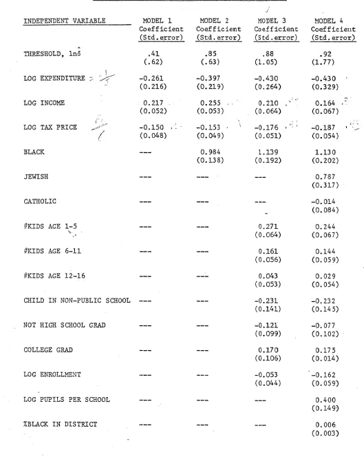
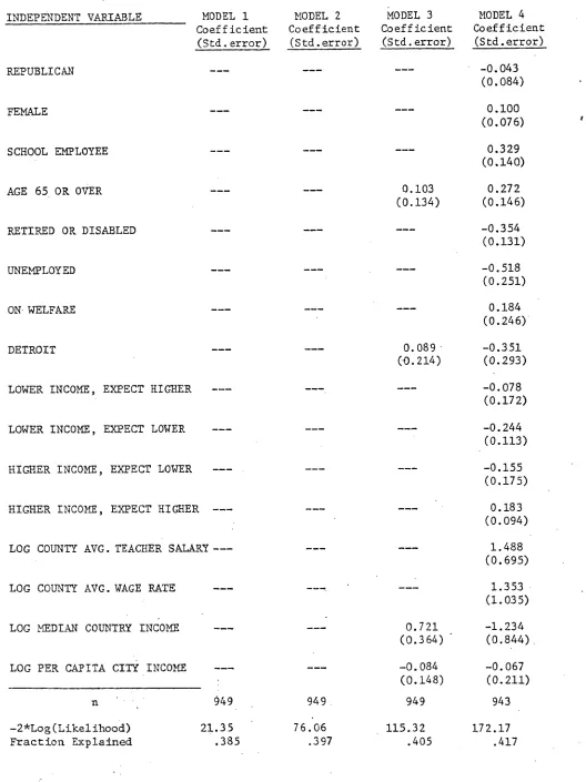
Table 1 presents our estimates of the coefficients in three alt- rnative specifications of a logit model. As observed in the previous discussion, the

coefficient of the variable "log expenditure" is our estimate of. the parameter,

1, while the coefficients of the other variables are estimates of _j where

S.

is the derivative of the elasticity of demand with respect to the

jth

In the appendix to this paper, tables A and B define the variables used and

Table 1. Demand Estimates -- Log it Formulation

INDEPENDENT VARIABLE MODEL 1 Coefficient (Std. error)

.41 (.62)

MODEL 2 Coefficient

(Std. error)

.85 (.63)

MODEL 3 Coefficient

(Std. error) .88 (1.05)

MODEL 4 Coefficient

(Std. error) .92 (1.77) THRESHOLD, 1n5

LOG EXPENDITURE -0.261

(0.216)

0.217 (0.052)

LOG INCOME

-0.397 (0.219) 0.255 (0.053) -0.153 (0.049) 0.984 (0.138) -0.430 (0. 264)

-0.430 (0.329)

0.164 (0.067) 0.210 .

(0.064) LOG TAX PRICE

BLACK

JEWISH

CATHOLIC

#KIDS AGE 1-5

7

-(0.048)

-0.176 (0.051)

1.139 (0.192)

"KIDS AGE 6-11

#KIDS AGE 12-16

CHILD IN NON-PUBLIC SCHOOL

NOT HIGH SCHOOL GRAD

COLLEGE GRAD

LOG ENROLLMENT

LOG PUPILS PER SCHOOL

%BLACK IN DISTRICT

Table 1, (con't.)

INDEPENDENT VARIABLE

REPUBLICAN ---.

FEMALE

--SCHOOL

EMPLOYEE---AGE 65 O R

OVER----RETIRED OR DISABLED

E

----

UNEMLYED--ON WELFARE

I

---DETRO

ITN---LOWER INCOME, EXPECT HIGHER

---LOWER INCOME, EXPECT ---LOWER

---HIGHER INCOME, EXPECT LOWER

----HIGHER INCOME, EXPECT ----HIGHER

---LOG COUNTY AVG. TEACHER

SALARY---.-LOG COUNTY AVG. WAGE RATE

---LOG MEDIAN COUNTRY INCOME

----LOG PER CAPITA CITY INCOME

----1 MODEL 2 MODEL 3

cient Coefficient Coefficient

rror) (Std.error) (Std.error)

0.103 (0.134)

0.089 (40. 214)

MODEL 4 Coefficient (Std. error)

-0.043 (0.084) 0.100 (0.076) 0.329 (0.140) 0.272 (0.146) -0.354 (0.131) -0.518 (0.251) 0.184 (0.246) -0.351 (0.293) -0.078 (0.172) -0.244 (0.113) -0.155 (0.175) 0.183 (0.094) 1.488 (0.695) 1.353 (1.035) -1.234 (0.844) . --0.067 (0.211) 943 172.17 417 D n

-2*Log (Likelihood)

Fraction Explained

-11-elasticity of demand are obtained by dividing the coefficients of "log income" and "log price" by the coefficient of "log expenditures".. These estimates and their estimated standard errors are reported in Table 2.

The first column of Table 1 reports estimated price and income elasticities of demand for local public education where the only explanatory variables used

are price and income. The survey data enable us to introduce a rich variety of additional explanatory variables which might have a substantial influence on

demand for education. The remaining columns of the table introduce successively more of these variables.

As more variables are added, one notices that the estimated income elasticity of demand falls. This is not surprising since several of the variables which are added are positively associated both with income and with demand for

educa-tion. For example, p-ople who have more education tend both to have higher incomes and, even controlling for income, to desire more expenditures on schools. In a demand equation including both education and income, the coefficient of income registers a "pure" income effect, holding education level constant. If education is not included, the coefficient on income has an additional component due to the effect that people with higher income tend also to be better educated

and better educated people like more money to be spent on education. Which type

of estimate is more appropriate depends on the purpose one has in mind. If one simply wants to know the extent to which the rich want to spend more than the poor do, then estimates based on equations excluding the education levels seem appropriate. If, however, one wants to predict the effect of a widespread

axogenous increase in income in the population, then controlling for the

educa-tion level and other characteristics of the voters would be more apt.

To us, most of the coefficients estimated seem plausible and consistent

-with a priori economic reasoning. One of the statistically strongest and, to us,

TABLE 2 DEMAND ELASTICITIES

Elastic it ies (Std. error)

MODEL 1 MODEL 2 MO DES, 3 MODEL 4 VARIABLE

INCOME 0.83

(0.74) -0.57

(0.54)

0.64 (0.40) -0.39

(0.26)

0.49 (0.34) -0.41

(0.30)

0.38 (0.34) -0.43

Table 3. Demand Estimates Using Alternative Tax Prices Model 2 -- Logit Formulation

Price 1

Coefficient

(Std. error)

Price 2 Coefficient

(Std. error)

Price 3 Coefficient

(Std. error)

Price 4

Coefficient

(Std. error)

Price 5 Coefficient

(Std.error)

INDEPENDENT VARIABLE

LOG EXPENDITURE1

LOG INCOME'

LOG

LOG HOUSE VALUE TAX PRICE2

LOG STATE AID TAX PRICE3

LOG CIRCUIT BREAKER PRICE4

LOG COMBINED PRICE5

DUMMY FOR CIRCUIT BREAKER4

BLACK'

n

-2*LOG(Likelihood) Fraction explained

-0.397 (0.219) 0.255 (0.053) -0.153 (0.049) -0.460 (0.216) 0.243 (0.056) -0.421 (0.212) 0.265 (0.055) -0.415 (0.224) 0.288 (0.066) -0.407 (0.224) 0.262 (0.068) -0.107 (0.052) -0.131 (0.047) -0.143 (0.056) 0.984 (0.138) 949 21.35 .385 0.996 (0.143) 970 69.96 .398 0.959 (0.145) 972 75.92 .398 0-287 (0.175) 1.018 (0.140) 941 73.48 .396 -0.092 (0.056) 0.189 (0.182) 1.000 (0.146) 916 70.71 .397

1_{LOG EXPENDITURE, LOG INCOME, LOG TAX PRICE, BLACK, as defined in Table 1A.}

2 reported market house value x assd.-to-market ratio in county, 1977

Tab Le J, (coil' L. )

3

LOG STATE AID TAX PRICE:

4

LOG CIRCUIT BREAKER PRICE;

to allow for the effects of state aid, price was adjusted for those respondents whose school district millage rate was less than 3% and for whom the value

(($40,000 - S.E.V. per pupil) x school millage rate) was greater than or equal

to zero, Price for these respondents was set equal to:

of

log _$40,000

Otherwise, price was kept at the value of "LOG TAX PRICE".

to adjust for the effects of the circuit-breaker program, price was set equal to 40% of its previous value for those respondents eligible, on the margin, for

the tax credit (corresponding to the 60% of taxes which are refunded). Specifi-cally, if the difference between the respondent's reported property taxes and 3.5%

of his income were greater than $0 and less than the maximum credit of $1200, his

price became:

(.4

Senior citizens eligible for the credit have the entire amount of their

property taxes refunded (up to $1200). For these respondents, price was set equal to one (ln(price) = 0) and a dummy variable for these respondents was

added to the equation.

It is a proxy for F(1-m)(1-b) where P is the tax price before state and or the circuit

breaker, m is the state and matching rate and b is the percent returned under the

circuit breaker. Again, for those senior citizens whose taxes are zero under the

circuit breaker, the log of this price is set equal to zero and a dummy variable

added to the equation (see footnote 4). SLOG OF CIRCUIT BREAKER

PRICE x STATE AID PRICE

TAX PRICE.

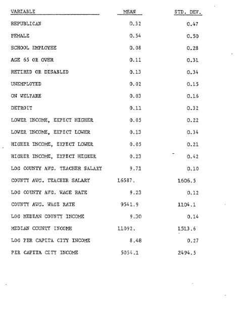
DESCRIPTIVE STATISTICS

Variable

LOG HOUSE VALUE TAX PRICE

HOUSE VALUE TAX PRICE LOG STATE AID TAX PRICE STATE AID TAX PRICE

LOG CIRCUIT BREAKER PRICE CIRCUIT BREAKER PRICE

CIRCUIT BREAKER DUMMY LOG COMBINED PRICE

COMBINED PRICE

Mean -0.66 0.65 -0.96 0.52 -1.21 0.42 0.09 -1930 0.40

Std. Dev.

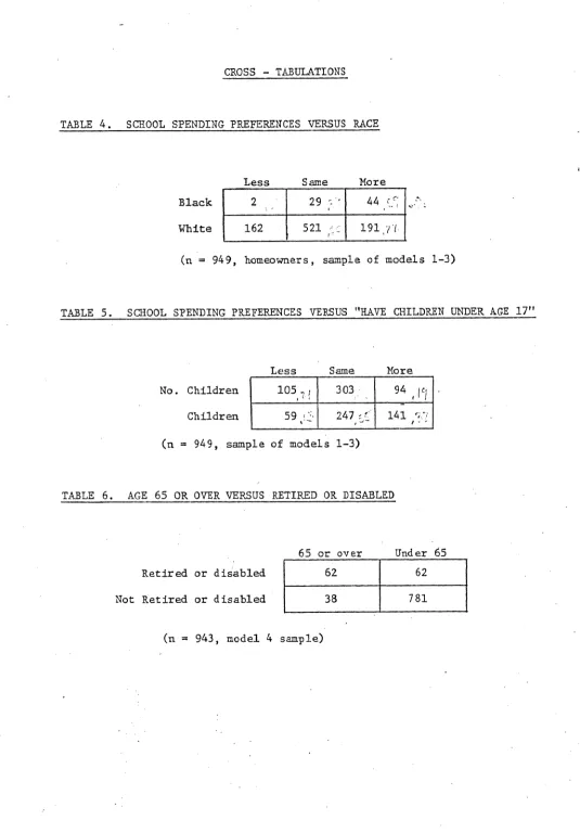
-12-cantly higher educational expenditures than do whites who have similar incomes

and tax prices. It is apparent from the raw statistics in Table 4 that blacks are much more likely than whites to favor an increa:e i4 expenditures in their school district. Furr

'

expenditures on local schools than are similar whites. .- 1y is this result

statistically significant and robust to changes in specifics- :a, the magnitude 15/

of this effect is very large.-- Perhaps there are special r sons why lacks' respond differently to interviews than whites. The fact that our study is

restricted to homeowners may provide misleading signals about black demands. For example, if black homeowners differ more radically from black renters in their demand for education than is the case for whites, then truncating our sample by homeownership will bias comparisons of black and white behavior. These possibili-ties are worthy of serious investigation, and we intend to look into them. Still it seems to us unlikely that we will explain away the strong differences found

here.

Our evidence also strongly -'ggests that Jews have higher demands for public education than other whi.as (but not so high as blacks). The demand of Catholics, when we control for the presence of children in non-public schools,

is insignificantly different from the demand of non-Catholics.

Among the most important variables affecting demand for public school expenditures, one would expect to find the number, age and enrollment status

of the respondent's children. From Table 5, it is clear that demands for

educational expenditure must be motivated by more than a narrow interest in thie

education of one's own children. From this table one sees that while people with

CROSS - TABULATIONS

TABLE 4. SCHOOL SPENDING PREFERENCES VERSUS RACE

Less Samte lore Black

White

(n = 949, homeowners, sample of models 1-3)

TABLE 5. SCHOOL SPENDING PREFERENCES VERSUS "HAVE CHILDREN UNDER AGE 17"

No. Children Children

(n = 949, sample of models 1-3)

TABLE 6. AGE 65 OR OVER VERSUS RETIRED OR DISABLED

Retired or disabled Not Retired or disabled

65 or over Under 65

62 62

38 781

-13-than is the case for people without children, only a quarter of. the respondents with no children of school age favor a reduction in expenditures on public schools.

People with children of preschool age may desire improvements in the school system with the anticipation that their children will soon begin a long period of schooling. People with children who have nearly completed school may regard

the benefits of an improvement in the school system as small since their children will soon be departing. As it turns out, our estimates show the effect on demand

of children aged 1-5 to be slightly larger than the effect of children aged 6-11. However, the coefficient on children aged 12-16 is significantly lower. Our

estimates imply that having a child aged 1-11 increases one's demand for education by about forty percent. Our coefficient estimates also suggest that having a

child in a non-public school can be expected to reduce one's demand for public education expenditures by about thirty percent. Since the number of respondents with children in non-public schools was small, the standard error of this

estimate is quite large.

Neither party politics nor sex seems to have much to do with voters demands for public education. Dummy variables stating whether the respondent

is female have numerically small and statistically insignificant coefficients. On the other hand, if a respondent or his spouse is employed by the local school district, his demand is about sixty percent higher than that of similar persons not employed by the school district.

In an attempt to account for differences between current and permanent income we asked respondents how their financial status had changed from five

years ago and how they expect it to change in the next f ive years . Thus we

have dummy variables for each of the situations:

1) worse now than in past,. expect better.

2) better now than in past, expect better.

-L4-4) better now than in past, expect worse.

It

as

income would be highest for answer (1) and successively lower for (2), (3) and (4). The permanent income hypothesis would then suggest a positive

co-efficients on (L) and (2) and negative coefficients on (3) and (4) with (1) having the highest and (4) the lowest coefficient. Lt turned out that (2) had a strong positive effect and (3) a strong negative effect, but (1) and (4) were

insignificant. This places our interpretation of the relation between these responses and permanent income in some doubt. On the other hand, it might be

that answers (2) and (3) indicate optimists and pessimists respectively while answers (1) and (4) suggest less decisive attitudes. Thus it might be that those who see steady improvement or steady: decline in their fortunes are the ones with

the greatest differences between current and permanent income.

It is interesting to see the effects of dummy variables for persons aged 65 or more and for whether the respondnet is retired or disabled. As can be seen -fromta Table 6, these are distinct groups. When one omits the variable "retired or disabled" the coefficient of age 65 is close to zero. However

when one includes this variable, our estimates suggest that people over 65

who are not retired or disabled want more excpenditures than people under 65,

(controlling, of course, for the effect of having children in school). Some-one who is over 65 and retired, however, would want slightly less than persons under 65. Unemployed respondents tended to want substantially Less

expendi-tures than the employed while recipients of welfare payments (ADC or food stamps)

tended to want slightly higher expenditures. Since the number of unemployed

and welf are rectpients in our sample was fairly small, however, the standard

errors on these estimates are large and the statistical significance of the

coefficients is

-15-district. One variable is total enrollment in the district. A second variable is the number of pupils per school in the district. Since larger districts may contain several schools physically separated from each other there seems

to be a problem analogous to the question of whether returns to scale accrue to the firm or the plant in a multi-plant firm. As it turns out, total district enrollment has a negative effect and enrollment per school in the district has a positive effect. We do not have: a good explanation for this result. If there were increasing returns to scale, then provision of equivalent education is cheaper in larger schools. Since the price elasticity of demand is estimated to be less than one in absolute value, the effect of increasing returns to dis-trict size would be to produce the observed negative coefficient on total enroll-.

ment. By the same token, if there were increasing returns to school size,

we should have expected a negative coefficient on the pupils per school variable. Instead we found a positive coefficient. Possibly this represents diseconomies of scale at the plant level. Alternatively this result nay be an artifact of some missing variables related to population density and urbanization.

We included as variables, mean per capita income in the city and in the county where the school district is located. This allows us to check whether there are neighborhood effects of some kind on individual demands. Such an

effect could never be disentangled in an aggregate study of the type we discussed previously and if such an effect appeared it would present a serious obstacle

to estimations based on aggregate data. As it turns out, the effect of city income is negligible. Although the variations in county income in the sample

were not large enough to give us a

very

left open that county income has some effect. One possible explanation for

such an effect is that county income differs l;:gely because of different,

-16-for local prices of school inputs and other goods. We have measures of average teacher salary and average wage rates in the private sector for the county in which each school district is located. The coefficient of average teachers' salary in the county is positive and significant. The coefficient of average wage in the private sector is positive, but not significant.

V. The Demands of Renters

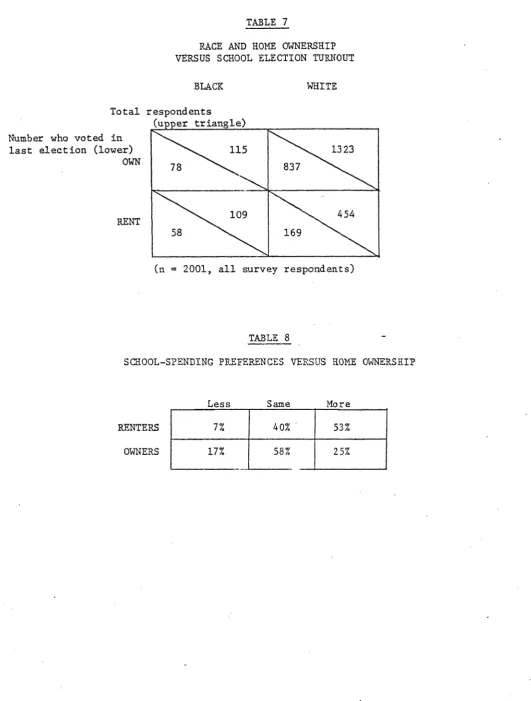
The results reported so far pertain only to the subsample of the Courant-Gramlich-Rubinfeld survey respondents who are homeowners. As Table 7 indicates, this omission excludes not only a substantial proportion of the total sample,

but also a similarly large proportion of the population that claims to have

voted in the last school election.

Thus it is clear that understanding the determinants of renter demands is important for understanding the outcome of school expenditure elections. Most aggregate studies suggest that, ceteris paribus, communities with a larger percentage of renters tend to spend more on public goods of all kinds. This suggests the likelihood that renters tend to vote for larger expenditure levels than homeowners. It is often argued that such voting behavior is due to a perception (whether correct or not) by renters that the tax cost of public goods is borne largely by their landlords. In the case of aggregate data, however, there remains the possibility that cities with a large percentage of renters have other unmeasured characteristics (perhaps urban congestion, high costs, or high crime rates) which lead both renters and owners to desire high expenditures and which creates the spurious inference that renters want to

spend more than homeowners. The survey results allow a direct comparison of the demand functions of renters and homeowners.

TABLE 7

RACE AND HOME OWNERSHIP VERSUS SCHOOL ELECTION TURNOUT

BLACK WHITE

Total respondents

Number who voted in last election (lower)

OWN

RENT

(upper triangle)

115 1323

78 837

109 454

58 169

(n = 2001, all survey respondents)

TABLE 8

SCHOOL-SPENDING PREFERENCES VERSUS ROME OWNERSHIP

Less Same More

RENTERS OWNERS

7% 40% 53%

r

-17-the demand functions of homeowners. The reason for this is that the

sub-sample of homeowners is "self-selected" from the sub-sample at large. Some of

the same variables which explain the demand of a respondent for local

expen-ditures might also influence his home ownership status. If this is so, our

estimated demand functions for homeowners might be biased by the non-random

selection for homeownership.

A conceptually difficult problem for estimating demand functions of renters

for public goods is deciding what is the appropriate tax price to use. There

is not wide agreement among economists about how the actual incidence of a property tax is divided between renters and owners. Even more problematic is deciding what a voter-renter perceives to be the effect of increased local government expenditures on his rental rate.

To a reasonable approximation, property taxes assessable against a rental unit are proportional to annual rents. Suppose that renters believed that some

fraction, possibly less than one, of the burden of property taxes falls on them in the form of higher rents. Then the tax price to a renter of local school

expenditures is proportional to the ratio of his annual rents to assessed value

per pupil in the school district where he resides. So long as this

proportiona-lity holds, the log-linear functional form allows us to estimate the price

elasticity of demand without knowing in advance. the fraction of taxes that renters

believe they pay. This is the case since using different values for this fraction 0

amounts to an equiproportional adjustments of tax price for all respondents. Thus our choice of a factor of proportionality would affect the intercept term but no t the ela stic ity of our f it ted r ent er d emand func tion. We have quit e

arbitrarily chosen to calculate tax prices as if renters pay a tax amounting to

17% of their annual r ent s. This is the f igur e used by the st at e o f Michig an

in its statewide property tax relief program. If a different fraction were used,

-18-would be different.

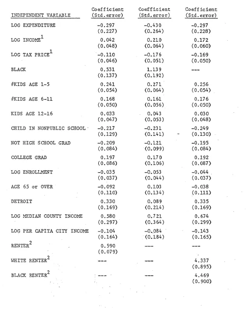
We see from Table 8 that renters are much more likely than owners to want higher expenditures than the current level in the school districts where they reside. In Table 9, we report the results of logit estimations for the entire population of respondents including both renters and homeowners, Columns 1 and 2 of Table 9 report these results with and without a dummy variable for renters. The large positive coefficient on the renter dummy strongly suggests that renters

tend to want higher levels of expenditure than homeowners who resemble them in

other respects.

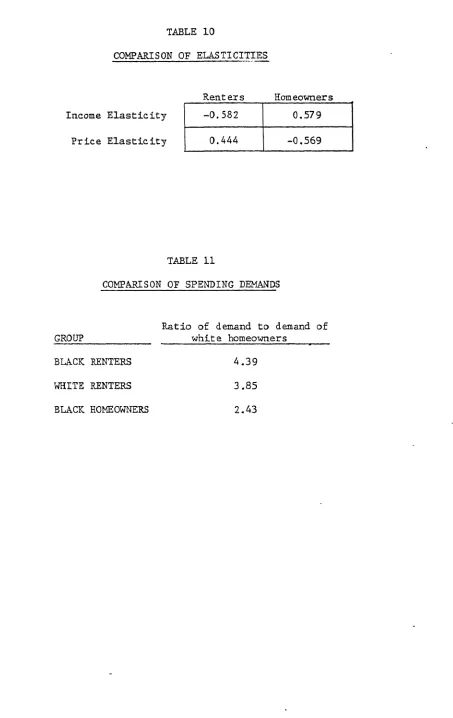
If our measured tax price for renters is proportional to the tax price that renters perceive, we should expect the price elasticities estimated for renters and homeowners to be approximately the same. To determine whether renters and homeowners have similar price and income elasticities of demand we

include interaction variables in the estimation reported in column 3. From

Table 10 we see that not only are the estimated price and income elasticities of renters different from those of homeowners, but they are of the "wrong" sign. We are thus led to believe that a satisfactory analysis of renter behavior will have

to draw its explanatory power from other variables than price and income as we

have measured them.

The estimates reported in column 3 of Table 9, allow different intercepts

for black renters, black homeowners, white renters and white -homeowners respectively.

In order to interpret these coefficients, we must allow for the fact that the renter variable is also interacted with price and income. In Table 11, we report

the estimated ratio of the quantity demanded by a member of each of the other

groups to the quantity demanded by a white homeowner if each of these individuals

has the mean income and faces the mean tax price for our sample. As we see,- black

renters want somewhat more than white renters and much more than black homeowners,

who in turn want much more than whith homeowners, We do not pretend to have

TABLE 9

Demand Estimates for Renters and Homeowners Logit Formulation

INDEPENDENT VARIABLE LOG EXPENDITURE

LOG INCOME1

LOG TAX PRICE1

BLACK

#KIDS AGE 1-5

#KIDS AGE 6-11

KIDS AGE 12-16

CHILD IN NONPUBLIC SCHOOL

NOT HIGH SCHOOL GRAD

COLLEGE GRAD

LOG ENROLLMENT

AGE 65 or OVER

DETROIT

LOG MEDIAN COUNTY INCOME

LOG PER CAPITA CITY INCOME

RENTER 2

WHITE RENTER2

BLACK RENTER

2

Coefficient (Std.error) -0.297 (0.227) 0.042 (0.048) -0.110 (0.046) 0.531 (0.137) 0.241 (0.054) 0.168 (0.050) 0.033 (0.047) -0.217 (0.129) -0.209 (0.084) 0.197 (0.086) -0.035 (0.037) -0.092 (0.110) 0.330 (0.169) 0.580 (0.297) -0.104 (0.164) 0. 590 (0.079)

Coefficient (Std. error)

-0.430 (0.264) 0.210 (0.064) -0.176 (0.051) 1.139 (0.192) 0.271 (0.064) 0.161 (0.056) 0.043 (0.053) -0.231 (0.141) -0.121 (0.099) 0.170 (0.106) -0.053 (0.044) 0.103 (0.134) 0.089 (0.214) 0.721 (0.364) -0.084 .(0.184) Coefficient (Std. error)

TABLE 10

COMPARISON

OF

Rent ers H~omeowners Income Elasticity

Price Elasticity

TABLE 11

CObIPARISON OF SPENDING DEMANDS

GROUP

BLACK RENTERS WHITE RENTERS BLACK HOMEOWNERS

Ratio

of

to

of

white

4.39 3.85

-19-VI. Comparison With Other Studies

It is of interest to see how our survey-based estimates compare with demand functions obtained from aggregate "behavioral" data. If demand functions

estimated from these two very different kinds of data yield similar results, credence is lent to both estimation methods. We would then have reason to hope that as evidence accumulates there may be some convergence of opinion on the nature of individual demand functions for public education.

In the literature on demand for public education there are several papers that measure price and quantity variables in a way that is at least roughly similar to our approach. In Table 12 we record all of the conceptually comparable

estimates of income and price elasticity that we have been able to find. The studies we list here all differ in at least minor ways, in their methods of

measurement and in the list of independent variables included in their estimations. Price elasticity, in particular, was measured in different ways in different

studies. As we have argued previously, the "price" that we would like to measure is the cost to a tax-payer of increasing per student educational inputs by one unit. This price

(4) t

(.)

(nH)

(p.)

i le i (A.V.

1-+M

where pE is the local price index for educational inputs, m is the matching rate on the margin from the state school aid program,

H

dis-trict where household i resides. Some of the authors were able to estimate Ti

directly from their data. Others had access to estimates of only some of the

f actors on the right side of (4) and had to treat the other factors as omitted

variables, with the hope that no bias would be ther eby introduced. Thus, for

-20-as -!-a. Many of the other researchers were able to estimate price as the product of two or more such factors. Feldstein, Ladd, and Lovett all allow the possibility that each of the four factors in the expression for price might have a different effect on total demand. Thus they each have r

-e

The estimated income elasticities in Table 12 are strikingly similar. Furthermore, our micro-based estimates are very close to most of the macro

estimates.-' Exceptions among the macro studkies are Peterson's estimates and our 17/

own macro based estimate of income elasticity.-- Despite the anomalies, we are impressed with the amount of independent evidence suggesting that the income elasticity of demand for local public education is on the order of 2/3.

The estimates of price elasticity in Table 12 are in less agreement than the estimates of income elasticity. This is no doubt partly due to the fact that different studies specified the price variable differently. The outliers in this

case are Feldstein's coefficient on matching aid and the coefficients for pupils per family found by Feldstein, Ladd, and Lovell. We have no explanation for the first discrepancy. The variable "pupils per capita", hovave, probably can not be satisfactixrily regarded as only a ptice variable in a :iacco study. It is true that the more pupils per capita there are, the more it costs the median voter to increase per student expenditure. It is also true that where there are more pupils per capita, a larger perc-_cage of the population has children in

school (as our micro data .how) are more likely to favor increased expenditures than people without children. The two effects work in offsetting directions and

for this reason it is not significa.ntly different from zero in the estimates of

Feldstein, Ladd, and Lovell. -- " The remaining estimat es of price are in rough

Table

12

Comparison of Estimaated Income and Price Elasticities

PRICE ELASTICITY ESTIMATES

________ ______ BASED ON: _ _ _ _ _ __ _ _ _ _

ESTIMATED INCOME ELAS TI CITY INESTGTOPR

%OF TAX BASE

1W01-RESIDENT:EAL

PUPILS PER

CkP ITA

STATE MATCHING

AID PATE

OTHiER

BASIS"

SA

OLE

Barlow 52 Urban .64 -. 34

M~ichigan (.10) (. 04) Districts

________

(1960)-Bradford- -5

58

dates~ Jersey (.08)

(.07)

District s 1 I/

(1960)

Brazer j1 40 large .73 -. 73

U.S. Cities (.34)

(.13)

(1953)

Feldsten

Ptown~s

(o1 .76) (.04) (.140)

(.18).0

(1970) (.07)

Inmian 58 Long .61 -4

Island (.11) .8

Districts (2970)

'Ladd , 78 Boston .46 -. 31

-.

03

SMSA (or .70)1)

(.25)

Districts (.15) (1970)

Lovell

~

Districts (.04) (.06)(14

(1970)

Peterson)'L See note .84 to 1.35-25o.7 below- (.10>).5

B-R-S Survey .64 -3

"Micro"- of

2,000

voters (1978)

B-R-S 469 Mich. .38 -1

"Macro" ;School,

(.03)

Districts

Notes on Table 12

1. Barlow, uses no variables other than "income" and "price". Barlow's income variable is family personal income per pupil in the comnunity, Most other

studies listed here use median family income.

2. Bradford and Oates use no variables other than "income" and "price". 3. Brazer measured expenditure as expenditure per capita in the community.

Most other researchers measured expenditure as expenditure per pupil, Brazer did not explicitly include a "price" term in his equation. However Brazer did include the ratio of pupils to population as an independent variable. We can therefore find the coefficients of the demand function

that Brazer would have found if he, like Bradford and Oates, had written his demand function with expenditures per pupil as a function of income and price. Since this transformation simply involves multiplying both sides of Brazer's equation by , the result ing equation has the same income elasticity which is equal to Brazer's coefficient on minus one. Brazer also included state aid for education and the ratio of 'ty to SMSA

population as independent variables.

IRES PUP

4. Feldstein obtains measures of the variables; A.V. ' N , as well as

.

dis-PUP 1

~A.V.rrr

cussion, he treats

1-M

(PE \(PUP\H r-^

with median income for his community will be t = 1 A. H where H is the value of his house. Thus it could be argued that the way in which PV should

enter the demand equation is through the tax price since T is inversely pro-portional to . _{Therefore tha negative of the coefficient on --V should}

A.V.

/PUP

be an estimate of the price elasticity of demand. We record this estimate under "other basis". When we look at the equation in this way, we notice that an important omitted variable in Feldstein's specification is H, median house value. We claim that omission of this variable biases the estimated income

elasticity downward. This can be seen as follows. According to most housing demand studies, the income elasticity of demand for housing is about one.

^h=^ [PE PUPk T^

Suppose, then that H =kY, for some k. Then t = 14m A.V. kY. Therefore the income elasticity estimated by Feld stein with the variable H omitted would be the sun of the ordinary income elasticity and the (negative) price elasticity. In Table 12 we record (in parentheses) the estimate of income elasticity obtained if one corrects for this effect by adding the absolute value of the estimated price elasticity to the estimated income elasticity.

Other variables in Feldstein' s specification include: "block-grant" state aid, f ederal grants, private school enrollment, and growth rate of school

5. Inman uses onl one price variable which is his estimate of the price

Ti = )H. The estimates reported here are from a specification

i1+M A.V.

that included only income, price and "state aid" as variables. Inman used a two stage least squares procedure to allow for possible effects of the

endogeneity of state aid.

6. Ladd's specification of variables is similar to Feldstein's. Our remarks on the Feldstein procedure apply here as well. In the case of Feldstein's

estimates, there were disturbingly large differences among the estimates

of price elasticity obtained from using each of the factors of price as an independent variable. Ladd's results are much more reassuring on this . account. The only coefficient substantially different from the others is that based on

(PN)

7. Lovell includes as independent variables, the factors ---

/,

\and()

P '

(A.V.

of the price term. We list his coefficient for - under, "other basis".

H

The estimates appearing in our table come from Column 1 of Lovell's Table 5. Of Lovell's several specifications, this one is closest conceptually to the others reported here. The parameter y reported in Lovell's Table can be

- shown to be very close to the income elasticity of demand. Lovell estimated

y = .65 and this is the income elasticity we report.

8. Peterson estimates five separate demand equations based on school expenditure

data in California, Michigan, New Jersey, New York, and-the Kansas City SMSA. All of his data is for years adjacent to 1970. Our Table 12 reports ,the range of his coefficients. Peterson's specification of the model differs from all

others treated here in that he uses locally raised revenue per student as

the dependent variable rather than total expenditure per pupil. Since total

expenditure per pupil is nearly equal to locally raised revenue per pupil plus state aid per pupil, and since Peterson included state aid as a variable, we should not expect this difference to affect the coefficients of variables

-21-demand somewhere between -1/4 and -1/2.

In Table 13 we summarize the estimated effects of a number of variables

other than price and income. Most of the macro studies suggest that renters favor greater expenditures than homeowners. This is strongly confirmed in our micro study. Education levels of parents are shown to have significant

positive effects on demand both in the micro and in the macro studies. Poverty status and political affiliation do not appear to be significant in either micro

or in macro studies. Race was not used as a variable in any of the previous macro studies. As it turned out, both our macro and our micro based estimates

suggest that cet paribus, b

eks

educa-tion than whites.

Our survey-based data enabled us to study the effects of many variables which are not readily measured from the usual data sources. This is illustrated by the fact that Table 13 includes ten interesting variables from our micro

study which were included in none of the macro studies. Furthermore, the micro nature of our data enables us to probe the structural relations between variables with more subtlety than is possible with macro data. For example, aggregate

studies can tell us the effect of the variable "number of school children as a fraction of the population". This variable is related to demand for "expenditure per student" both through a price effect and through the fact that in districts

where there are more children per capita, more families have children of their own

and hence value educational expenditures ,.:re highly.' Only with micro data are we able to disentangle these two effects in a reasonable way. We know for each

of our respondents whether he has children of his own in public school and the

tax price he pays per dollar of per student expenditure. Similarly, aggregate demand studies can relate expenditure per student to the percentage of children

of school age who attend private schools. However, it is possible that districts

Table 13

Effects

of

other

STUDY BR-

--VARIABLE FLSU

~4N

MICRO

%Non-White 4+ +

%Renters 0 4++4- +

%Old- 0 +

Educat ion

of Parents

Catholic 0 0

Childr en in 0

Private School

Democrat 0 0

Poverty0 0 0

Childr en +

Under 5

Childr en +

Over 5

Jew~.ish 4+

S ex 0

School +

Employee

Retired

orT

Disabled Unemapl.oy

-22-from the average district so that estimates of the effect of private school

enrollment are contaminated. Our data enable us to determine whether each respondent sends his own children to private school. A similar observation applies to the case of renters, blacks and the aged.

PostScript

We have demonstrated a method for estimating individual demand functions from individual qualitative responses to a survey. This leads to estimates of income and price elasticities of demand for local school expenditure that are similar to those obtained in aggregate studies using "median-voter" models. The fact that similar estimates are derived from two very different

kinds of data lends some support to the validity of both approaches.

Although survey data are typically much more expensive to- obtain than the

data for cross-sectional median-voter studies, a survey does enable one to obtain

a richness of detail about voter characteristics that seems unobtainable

from other sources. We have attempted to convey some of this richness in

our reported results. For example, our results indicate that on the average one is more likely to desire higher expenditures on local public education if one is black, Jewish, a renter, a college graduate, a school employee, if

one has children in public schools or if one is over 65 years old. One is more likely to demand lower expenditures if one has children in private school or is

retired, disabled or unemployed. Variables which might have mattered but appear to be insignificant are political party affiliation, sex, lack of a high school education, and Catholicism. We do not pretend to have adequate

explanations for all'of these results, nor to have pursued all of the inter-esting possibilities for interpretation. It is our hope that this paper will

help ethers to advance empirical knowledge about preferences for particular

public goods, both through collection of more evidence and through

Footnotes

1/

- The individualistic theory of efficient provision of public goods dates at least from the work of Wicksell (1896) and Lindahl (1919). Its definitive treatment in modern terms is found in Samuelson (1954). A positive theory, relating outcomes in democracies to voter preferences was developed by Bowen (1943). Other contributions to this tradition include Black (1958), Downs (1957), Buchanan and Tullock (1962), and Barr and Davis (1966), Barlow (1970), and Bergstrom (1979).

2/

- Some might wonder whether it is appropriate to treat education as a Samuelsonian "pure public good". The operational content of our treatment is simply this. Each respondent in the sample is assumed to have a utility function that depends on an index of the quality of education offered to students in his district and on his expenditures on "all other goods". The index of quality used in this

paper is total expenditures per pupil. In the appendix we discuss the appropriate-ness of this index in some detail.

3/

- A critique of the "median voter model" is found in Romer and Rosenthal (1979). 4/

- Examples of research of this kind are Deacon and Shapiro (1975) and Neufeld (1977).

5/

- The paper which comes closest to doing this is Gramlich and Rubinfeld (1980).

The authors estimate demand functions of individuals for total spending in their county of residence. The methods used in that paper are quite different from those used here.

6/

- Many economists view inference from survey results with suspicion. Often this attitude is justified. For example, if a survey asks a consumer how he would behave in situations that are remote from his normal experience, his

answer may be very different from the behavior he would actually choose if he had time to consider carefully or perhaps experiment with responses to the hypothetical situation. Some surveys, (knowingly or not) ask attitudinal

ques-tions where th