14th International Conference on Wireless Communications, Networking and Mobile Computing (WiCOM 2018) ISBN: 978-1-60595-578-0
Diffusion Clustering Routing Protocol (DCRP) in Wireless
Sensor Networks
Yinghong Liu1 and Yuanming Wu2,*
3
ABSTRACT
With the popularity of wireless sensor networks (WSNs), it is high time to solve the tough problem of isolated nodes. To avoid isolated clusters effectively, we proposed Diffusion Clustering Routing Protocol (DCRP). In this scheme, clusters are diffusing outward from the base station (BS) hop by hop. BS and the one-depth sensor nodes form the first cluster and then new cluster heads (CHs) are selected from the member nodes of existing clusters. Moreover, the optimal CHs equation (1) consist of three factors of the number of neighbor nodes, depth and residual energy. DCRP realizes the communication between neighbour CHs without the help of relay nodes and makes energy consumption equilibrate among CHs during data transmission, prolonging the lifespan of WSNs with low transmission delay. Table 1 shows that DCRP extends the lifespan of WSNs by 65%, 16% and 10% respectively compared with DEBR, EEUC and MOCH.
KEYWORDS: wireless sensor networks; diffusion clustering routing protocol, isolated CHs; lifespan of WSNs
I. INTRODUCTION
Wireless sensor networks (WSNs) consist of a large number of sensor nodes, capable of sensing, computing, and wireless communication [1]. Usually, theses nodes monitor specific targets and collect data, and then send data packets to a sink or the base station (BS) with wireless transmission techniques [2-3].Obviously, isolated nodes can bring the loss of data and other unpleasant troubles.
The off-the-shelf clustering algorithms, such as DEBR [4], LEACH [5] and its variants [6-9], DEEC [10], MOCH [11], become not applicable due to the unavoidable occurrence of isolated cluster heads (CHs). With the help of relay nodes, clustering algorithms like EEUC [12], have solved this problem but only for the time being. That is because relay nodes consume more energy than other member
1
School of Automation Engineering, University of Electronic Science and Technology of China
2
University of Electronic Science and Technology of China; No. 2006, Xiyuan Ave, West Hi-Tech Zone, 611731, Chengdu, Sichuan, P.R. China
nodes to deliver the packets of isolated CHs, and as a result, they may die earlier and generates isolated island.
In [11], the Markov chain model is proposed to select the optimal number of clusters in the network based on the distribution of CHs in every round. The average selected CHs in every round, SD (Standard deviation) of the number of CHs and COV(Covariance) of the number of CHs are taken into account to ensure the uniform cluster members and even load, which can achieve optimal resource utilization. Within the framework of this design, the author also set a range to limit the number of CMNs (Cluster Member Nodes) in the cluster to allocate energy cost.
As for DCRP, it is a brand new clustering algorithm. Different from the above methods, DCRP aims to prevent generating isolated CHs with no relay nodes. Meanwhile, DCRP equilibrates the energy consumption among transmission nodes to prolong the lifespan of WSNs, and minimizes the number of clusters to guarantees short transmission delay.
The rest of this paper is organized as follows. In section II, we elaborate DCRP in detail. In section III, we discuss the calculation of CHs number and energy consumption. In section IV, we give the simulation and evaluation of DCRP. In section V, conclusions are drawn out.
II. DETAILS of DCRP
A System Model
Without loss of generality, we assume that N sensor nodes are deployed in an M×M square region randomly and uniformly. All the sensor nodes are stationary and BS is in the center of the square field. In order to simplify the analysis process, we make assumptions as follows.
1. All the sensor nodes are homogeneous of limited energy; 2. The communication radius of each node is R;
3. Each node has a unique identity ID.
To calculate the energy dissipation of sensor nodes, we use the radio energy dissipation model [13-14] which is widely used by the majority of researchers.
B Definitions
To illustrate our routing scheme clearly, we give some basic term definitions.
One-depth nodes: The one-depth nodes are the nodes which can communicate with BS directly.
Neighbor Nodes Out of Cluster: The neighbor nodes out of cluster of node i are the nodes within the transmission radius of node i, but not in a certain cluster. We use N(i) to represent the number of neighbor nodes out of cluster of node i.
CH Depth: The depth of CHs which can communicate directly with base station is defined as one. The depth of CHs that can communicate with one-depth CHs outward from BS is two, and the depth of other CHs can be deduced in the same way. We use D(i) to represent the depth of CH i. In addition, the depth of a node or a cluster is equal to that of its CH.
Parent CH: The parent CHs of CH i are the CHs whose depths are one less than that of CH i.
Child CH: The child CHs of CH i are the CHs whose depths are one more than that of CH i.
Network Lifespan: The network lifespan is the lifespan of all the one-depth nodes.
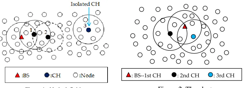
As shown in Figure 1, CH1 can communicate with BS directly and its depth is one. CH2 is selected from the member nodes of CH1, so we call one-depth CH1 CH2's parent CH and call two-depth CH2 CH1's child CH inversely. The nodes, in the dotted circle but out of cluster 1, are CH2's neighbor nodes out of cluster. Having no neighbor CHs within its transmission radius, CH3 is an isolated CH.
C The Cluster Head Selection Strategy
In the cluster-based routing protocols, the selection strategy of CHs is of essential importance. And this part is the highlight of DCRP! Here, we have
𝑊(𝑖) = 𝛼𝑁𝑁(𝑖)
𝑚𝑎𝑥+ 𝛽
1 𝐷(𝑖)+ 𝛾
𝐸(𝑖)
𝐸0 (1)
In equation (1), N(i) is the number of neighbor nodes out of cluster of node i.
𝑁𝑚𝑎𝑥 is the maximum N(i). D(i) represents the depth of node i. E(i) is the residual energy of node i and E0 is the initial energy of each node. To make sure the value of
𝑊(𝑖) is between 0 and 1, we let 𝛼 + 𝛽 + 𝛾 = 1.
Figure 1. Node definitions. Figure 2. The clusters.
D Cluster construction phase
In this phase, BS and the one-depth nodes becomes the first cluster where BS is assumed to be the CH. The member nodes of the first cluster transmit clustering packets to BS. BS processes the received packets and then broadcasts a packet of the new CH to all one-depth nodes. All the CHs will be produced in the same way. The cluster construction phase is over until each sensor node joins a certain cluster. The procedure can be divided into following steps :
Step 1: BS first broadcasts a start-signal to tell all the nodes that the cluster construction phase begins and then each node estimates the distance from BS according to the received signal intensity. BS and nodes in its R radius form the first cluster where BS is taken as a CH. The CH depth of BS is defined as one.
Step 2: The member nodes of the first cluster send a broadcast signal to obtain the number of their neighbor nodes out of cluster and save it in their clustering packets and then send the clustering packets to BS. After receiving the clustering packets, BS extracts the depth, residual energy and the number of neighbor nodes out of cluster of each candidate node. Then BS computes the value of each member node's W(i), stores them and chooses the node which has the maximum W(i) to be the next CH. This new CH and all its neighbor nodes out of cluster form the second cluster. The depth of the new CH is two.
Step 3: The member nodes of the second cluster transmit clustering packets to their CH and then the packets are sent to BS through the parent CH. BS computes the W(i) values of all new member nodes and compares them with that of other member nodes. The node which has the maximum value of W(i) will become the third CH. The third CH and its neighbor nodes out of cluster form the third cluster. Figure2 shows the example of the first cluster, second cluster and third cluster.
Step 4: Repeat step 3 until all the CHs and clusters are generated and all sensor nodes have joined their clusters.
: 3rd CH : 2nd CH
[image:4.612.132.529.88.232.2]E Data transmission phase
The multi-hop transmission mechanism is used in WSNs because of the low communication ability of nodes with constant transmission power. Regarding a cluster as an ordinary node of a tree and BS as a root node, the process of clustering is like the course of generating tree. Data transmission starts with the leaf nodes and then CHs send the data to base station hop by hop. The whole process is as follows:
Step 1: BS broadcasts a start-signal to tell all the nodes that the data transmission phase begins. All of the cluster member nodes collect data and then send the data to their CHs. After aggregating and compressing data, CHs transmit them to the parent CHs.
Step 2: The outer layer data is delivered to BS hop by hop. The data delivery of that cluster chain is over, till they arrive at BS. If a CH has more than one parent CH, the CH will forward the data to the one with the least depth.
Step 3: Repeat step 1 and step 2 until any one of one-depth node consumes more than 20% of initial energy. Where after, the data transmission phase of this round is over and the cluster construction phase of next round will begin.
To avoid routing loop and redundancy, the energy-balanced loop-free routing algorithm [15] is used in data transmission phase. In this algorithm, a route line field is set to keep an account of the nodes’ address passed in data packets, which can reduce transmission delay and unnecessary energy consumption, as well as a mixed three-dimensional field in terms of depth, energy density and residual energy is constructed, which can achieve global energy balance.
III. CHs NUMBER AND ENERGY CONSUMPTION
A Number of CHs
In DCRP, we set the communication radius of nodes to R (100m), so the coverage area of a cluster is 𝜋𝑅2. When the cluster construction phase is finished, the coverage area of all clusters is supposed to be around the network size (1000m×1000m). If there are n clusters, we have
𝜋𝑛𝑅2− 𝑆
𝑜𝑣𝑒𝑟𝑙𝑎𝑝 ≈ 𝑆𝑛𝑒𝑡𝑤𝑜𝑟𝑘 (2)
where the 𝑆𝑜𝑣𝑒𝑟𝑙𝑎𝑝 is the overlapping coverage area, and the 𝑆𝑛𝑒𝑡𝑤𝑜𝑟𝑘 is 1000m×1000m. When two rounds intersect, the intersecting area
𝑆 = 2𝑅2𝑎𝑟𝑐𝑐𝑜𝑠 (𝑑
2𝑅) − 𝑑√𝑅2− 𝑑2
where d is the distance of the two centers of circles, like the distance of a cluster head and its parent cluster head. Since the nodes are uniformly and randomly distributed in network ,we can calculate the mathematical expectation of d that is
𝐸[𝑑] = ∫ 𝑥𝑓(𝑥)𝑑𝑥0𝑅 = ∫ 𝑥 (𝑅𝑥22)
′
𝑑𝑥 =2𝑅3
𝑅
0 (4)
Put 𝐸[𝑑] into (3) and we can get S ≈ 1.83R2. Estimate Soverlap= (n − 1)S, therewith 𝑛 ≈ 75. So the number of cluster heads is around 75, and it will be verified in part C, section IV.
B Energy Consumption of DCRP
For our experiments, we set R (communication radius of nodes) 100 meters, and then the energy dissipated in all cluster head nodes during a round is
𝐸𝐶𝐻 = (𝑁 − 𝑚)𝐸𝑅𝑥(𝑘) + (𝑁 − 𝑚)𝐸𝐷𝐴+ 𝑛𝐸𝑇𝑥(𝑘, 𝑑𝑡𝑜−𝑝𝑎𝑟𝑒𝑛𝑡𝐶𝐻) (5)
Here, k is bits of packet, 𝑛 is the number of CHs, m is the number of one-depth CHs, 𝑁 is the number of all nodes, 𝐸𝑅𝑥(𝑘) is receiving energy consumption, 𝐸𝐷𝐴 is the energy consumption of data aggregation and 𝐸𝑇𝑥 is transmission energy consumption. The coeffiient of ERx(k) and EDA are N-m, because all cluster heads except one-depth cluster heads receive data not only from their non-cluster head member nodes but also their child CHs.
The energy consumption in all cluster member nodes during a round is
𝐸𝑛𝑜𝑛−𝐶𝐻 = (𝑁 − 𝑛)𝐸𝑇𝑥(𝑘, 𝑑𝑡𝑜𝐶𝐻) (6)
where
𝐸𝑇𝑥(𝑘, 𝑑) = 𝑘𝐸𝑒𝑙𝑒𝑐+ 𝑘𝜀amp𝑑4 (7)
𝐸𝑒𝑙𝑒𝑐 𝑎𝑛𝑑 𝜀amp are from energy consumption model of nodes in [15].The total energy consumption in a round is
𝐸𝑡𝑜𝑡𝑎𝑙−1𝑟𝑜𝑢𝑛𝑑 = 𝐸𝐶𝐻 + 𝐸𝑛𝑜𝑛−𝐶𝐻 (8)
In DCRP, cluster heads are also member nodes of their parent cluster heads, so in statistics we have 𝑑𝑡𝑜−𝑝𝑎𝑟𝑒𝑛𝑡𝐶𝐻= 𝑑𝑡𝑜𝐶𝐻. In general, 𝐸𝐷𝐴 is ignored, so
IV. SIMULATION RESULTS AND ANALYSIS
In this section, we describe the simulations evaluating the performance of DCRP. For simplicity, an ideal MAC layer and error-free communication links are assumed.
A Simulation Environment
500 homogeneous sensor nodes are deployed randomly and uniformly in a square area of 1000m×1000m with BS at (500m, 500m). The initial energy of each node (E0) is 0.5J and communication radius of each node (R) is 100m. Eelec, εfs and εmp are respectively 50nJ/bit, 10pJ/bit/m2 and 0.0013pJ/bit/m4.
B Value of 𝑵𝒎𝒂𝒙
𝑁𝑚𝑎𝑥 is the maximum number of neighbor nodes out of cluster. To get the value of 𝑁𝑚𝑎𝑥, we let W(i)=N(i).The result is shown in Figure 3 and Nmax is 14. According to calculation, the mean value 𝐸[𝑛(𝑖)] is 7 and standard deviation
√𝐷[𝑛(𝑖)] is 3.49.
C Values of 𝜶, 𝜷 and 𝜸
[image:7.612.308.480.503.644.2]Setting the values of α and β between 0.2 to 0.6, several representative results are shown in Table I. As we can see, the number of cluster heads is around 75, and the optimal values of α, β and γ are respectively 0.5, 0.3 and 0.2.
TABLE I. VALUES OF α, β AND γ.
Different values of α, β and γ Mean number of clusters Mean depth of CHs
α= 0.3,β= 0.4,γ= 0.3 76.6 5.98
α= 0.5,β= 0.3,γ= 0.2 72.8 6.37
α= 0.4,β= 0.4,γ= 0.2 75.3 6.34
α= 0.3,β= 0.5,γ= 0.2 77 5.96
α= 0.6,β= 0.2,γ= 0.2 72 6.73
α= 0.4,β= 0.3,γ= 0.3 74.8 6.47
D Performance Analysis
Network lifespan and transmission delay are two vital performance parameters. In DCRP, the nodes with more residual energy, less depth and more neighbor nodes out of cluster be more likely to become CHs. Therefore, the energy consumption of the whole network is balanced and the mean depth of CHs is minimized. As a result, DCRP expands the network lifespan and shorten the transmission delay. In DEBR, each sensor node maintains an adjacency list where the hop numbers and residual energy of its neighbor nodes are saved. Nodes forward packets to nodes of less hops and more residual energy. Therefore, DEBR performs better in energy balance than other homogeneous algorithms. In EEUC, CHs are selected by considering the residual energy of nodes and the distance between nodes and the edge of the annular region. A cluster size optimization formation algorithm is used to produce clusters in descending order of the size of the cluster, making the energy consumption of the whole network balanced. Therewith, EEUC can prolong the network lifespan. However, EEUC cannot avoid producing isolated CHs and must use relay. In MOCH, BS calculates the optimal number of cluster heads to ensure even energy distribution in the network, but this may not be applied in the network composed of sensor nodes with constant transmission power. These are the state-of-the-art research achievements and they perform better in network lifespan and transmission delay than other homogeneous methods. Here, DEBR, EEUC and MOCH are taken into comparison with DCRP in our simulation experiments.
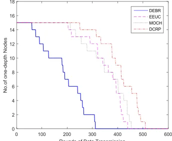
We can tell from Figure 4 that, when there are 500 sensor nodes in total, four methods all have 15 one-depth nodes and respectively 311, 439, 454 and 509 rounds of data transmission. Easily, we can get that DCRP prolongs the network lifespan by 65%, 16% and 10% compared with DEBR, EEUC and MOCH.
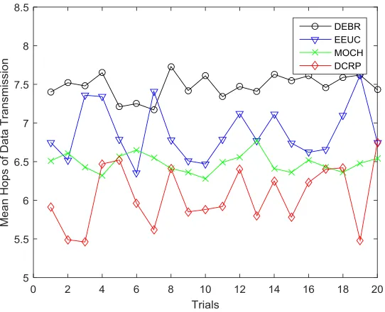
Figure 5. Transmission delay.
V. CONCLUSIONS
In proposed DCRP, we construct clusters in the manner of diffusing outward centered on BS. All the new CHs are selected from the member nodes of existing clusters so that we can guarantee that there is at least one neighbor CH within the communication radius of each CH. Thus, isolated CHs are avoided. In the CH selection strategy, we construct a weight function in which the residual energy, depth and the number of neighbor nodes out of clusters are taken into consideration. This strategy can balance the energy consumption of CHs, improve the energy efficiency and lower the transmission delay. Thus, the network lifespan is prolonged. Analyses and simulation results show that DCRP ensures no isolated nodes and prolongs the lifespan of WSNs by 65%, 16% and 10% respectively compared with DEBR, EEUC and MOCH.
ACKNOWLEDGMENTS
REFERENCES
1. Corke, P.; Wark, T.; Jurdak R. Environmental wireless sensor networks. Proceedings of the IEEE. 2010, 98, 1903 - 1917.
2. Muhammad, I.; Muhammad, N.; Alagan, A. Wireless sensor network optimization: Multi-objective paradigm. Sensors. 2015, 15, 17572-17620.
3. Akhtaruzzaman, M.A.; Mohammad, A.R.; Ishtiaque, A. Bio-mimic optimization strategies in wireless sensor networks: A survey. Sensors. 2014, 14, 299-345.
4. Lu, W. Distributed energy balancing routing algorithm in wireless sensor networks. Springer Berlin Heidelberg. 2012, 127, 227-232.
5. Heinzelman, W.; Chandrakasan, A.; Balakrishnan, H. Energy-efficient communication protocol for wireless micro sensor networks. In Proceedings of the 33rd Annual Hawaii International Conference on System Sciences. Maui, HI, USA, January 2000, 2, pp. 4–7.
6. Heinzelman, W.B.; Chandrakasan, P.; Balakrishnan, H. An application-specific protocol architecture for wireless micro sensor networks. IEEE Transactions on Wireless Communications. 2002, 1, 660–670.
7. Xu, Z.Z.; Chen, L.Q.; Liu, T. Balancing energy consumption with hybrid clustering and routing strategy in wireless sensor networks. Sensors. 2015, 15, 26583-26605.
8. Younis, O.; Fahmy, S. HEED: a hybrid, energy-efficient, distributed clustering approach for ad hoc sensor networks. IEEE Transactions on Mobile Computing. 2004, 3, 366–379.
9. Handy, M.J.; Haase, M.; Timmermann D. Low energy adaptive clustering hierarchy with deterministic cluster-head selection. in: Mobile and Wireless Communications Network, 2002. 4th International Workshop on, Stockholm, Sweden, September 2002, pp. 368–372.
10. Qing, L.; Zhu, Q.X.; Wang, M.W. Design of a distributed energy-efficient clustering algorithm for heterogeneous wireless sensor networks. Computer Communications. 2006, 29, 2230–2237.
11. Ahmed, G.; Zou, J.H.; Zhao, X. Markov chain model-based optimal cluster heads selection for wireless sensor networks. Sensors. 2017, 17, 440-469.
12. Peng, D.; Li, S.; Yang, X. An energy efficient uneven cluster-routing protocol for wireless sensor networks. Chinese Journal of Sensors & Actuators. 2014, 27, 1687-1691.
13. Wen, Y.Y.; Gao, R.; Zhao, H. Energy efficient moving target tracking in wireless sensor networks. Sensors. 2016, 16, 29-43.
14. Liao, S.K.; Lai, K.J.; Tsai, H.P. Distributed information compression for target tracking in cluster-based wireless sensor networks. Sensors. 2016, 16, 937-960.