2019 2nd International Conference on Informatics, Control and Automation (ICA 2019) ISBN: 978-1-60595-637-4
Study on Separation of Underwater Vehicle Noise
Based on Blind Source Separation
Xiao-bo NIU
1and Guo-qiang FU
21
Naval Petty Officer Academy, Bengbu, China
2
Beijing Aerospace Unmanned Vehicles System Engineering Research Institute, Beijing, China
Keywords: Blind source separation, Kernel independent component analysis, Underwater vehicle.
Abstract. Aiming at the study of underwater vehicle noise extraction in the measurement, a method based on blind source separation (BBS) is presented, and the kernel independent component analysis (KICA) is used in the separation of underwater vehicle noise. The principle and algorithm is introduced and the simulation is carried on to compare with the traditional ICA algorithm in BBS. The simulation results show that KICA not only separates the underwater vehicle noise effectively but also is more accurate than the traditional ICA algorithm.
Introduction
Underwater vehicle shock absorption and noise reduction is a hot topic in many countries, while how to improve the noise test level of underwater vehicle is an important means of noise reduction. The navigational radiation noise of an underwater vehicle is mainly composed of machinery noise, propeller noise and hydrodynamic noise [1]. The vibration of internal mechanical equipment of the underwater vehicle that radiates into the seawater through vibration or excitation of vehicle hull is called machinery noise. Propeller noise is the noise generated by the propeller rotating in seawater, including propeller cavitation noise, propeller rotation and blade vibration. Hydrodynamic noise is the noise generated by the relative motion of the surface of the vehicle hull and the aqueous medium during navigation by the underwater vehicle.
A variety of methods are adopted to comprehensively analyze and identify noise sources, to effectively identify the distribution of major noise sources and separate the contribution of machinery noise, hydrodynamic noise and propeller noise to radiation noise. Therefore, it is of great significance to obtain the overall acoustic performance of the ship under test and evaluate the noise design indexes for noise control. So, how to separate the data of different noise sources from the acquired data is an important research content.
Blind Source Separation and Kernel Independent Component Analysis
Independent component analysis (ICA) is a typical blind source separation method. Its essence is to blind source separation of multi-channel observation signals under the assumption of statistical independence and dig out independent source components hidden in the observation signal [2]. In 2002, F. R. Bach, M. I. Jordan et al. introduced the idea of kernel function on the basis of traditional ICA theory, and proposed a new type of ICA algorithm: Kernel Independent Component Analysis (KICA) [3] to further improve the separation effect.
Basic Principles of Kernel Independent Component Analysis
Kernel independent component analysis is not a combination of existing independent component analysis and kernel function, but a new method. The idea is to use nonlinear mapping :RN R to
inner product operation between two input vectors to realize nonlinear transformation in Reproducing Kernel Hilbert Space. Therefore, it is not necessary to construct specific nonlinear expectation function.
Mercer Kernel
Any function that meet Mercer's condition can be used as Mercer kernel and decomposed into dot product form in feature space [4] The Mercer condition can be described as Eq. 1 for any
square-integrable function:
0 )
( ) ( ) , (
2 1
LL K x y g x g y dxdy (1) Some common Mercer kernel functions include:Polynomial kernel:
d y x y x
K( , )( 1) , d is a constant (2)
Gaussian kernel:
2 2
2 ) ( exp ) , (
y x y
x
K
, 0 (3)
Kernel Independent Component Analysis Algorithm (KICA Algorithm)
Let x1,x2RN, Fis a function vector space from R to R, and the correlation coefficient F of x1
and x2 is defined as the maximum correlation coefficient between the random variable f(x1) and )
(x2 f
2 / 1 2 2 2 / 1 1 1
2 2 1 1
2 2 1 1
)) ( (var )) ( (var
)) ( ), ( cov( max
)) ( ), ( ( max
2 2
2 2
x f x
f
x f x f
x f x f corr
F f f
F f f F
(4)
F
is a comparison function between random variables. Obviously, if x1andx2 is independent, thenF 0. If the space Fis large enough, the opposite is true. The idea of Reproducing Kernel Hilbert Space [5] is used to calculate theF. Let F to be the Reproducing Kernel Hilbert Space on the real number set. K(x,y) is a kernel associated with this space. Let (x) K(,x) as a mapping from the input space to F , K(,x) is a functional function with x as the variable in F space. With regeneration characteristics of kernel Hilbert space [6]:
f x x
f( ) ( ) ,f F,xR
(5) Then,
1 1 2 2
2 2 1
1( ), ( )) ( ) , ( )
(f x f x corr x f x f
corr
Let
x x x1N
21 1
1, ,, and
N x x
x 2
2 2 1
2, ,, to be the vectors composed of N observation values of
random variable x1 x2 respectively.
( ), ( ), , ( 1 )
2 1 1 1
N x x
x
and
( ), ( 2), , ( 2)
2 1 2
N x x
x
are the
function values of F . Assuming that they have been centralized, i.e., ( ) ( ) 0
1 2 1
1
N
i i N
i i
x
x . Then,
2 / 1 2 2 2 2 2 / 1 1 2 1 1 2 2 1 1 2 1 ) ( ) ( max ) , ( 2
1 a K a a K a
a K K a K
K T T
T R a a F N (6) Solving the above formula is equivalent to solving the following formula:
2 1 2 2 2 1 2 1 1 2 2 1 0 0 0 0 a a K K a a K K K K (7) Where, K1 and K2are the Gram matrices of the observed data, a1a2are the eigenvectors of K1and
2
K respectively. Eq. 7 can be extended to multiple variables:
m m m m m m m m m a a a K K K a a a K K K K K K K K K K K K K K K K K K 2 1 2 2 2 1 2 1 2 1 2 2 2 1 2 1 2 1 1 1 0 0 0 0 0 0 (8)
Algorithm Steps of KICA
t x t x
tx1 , 2 ,, M are M observation vectors for mixed signals, K(x,y)is a predetermined kernel function, Wis a randomly generated initialization decomposition matrix.
Step 1: The observed data was undergone whitening process;
Step 2: LetY WX, obtain the estimated value y1,y2,,yN of the source signals1,s2,,sN, and
calculate the estimated Gram matrix K1,K2,,KN of estimated value by Cholesky decomposition;
Step 3: Defined as the maximum eigenvalue of the following formula:
m m m m m m m m m a a a K K K a a a K K K K K K K K K K K K K K K K K K 2 1 2 2 2 1 2 1 2 1 2 2 2 1 2 1 2 1 1 1 0 0 0 0 0 0
(9)
Step 4: Set the objective functionC W logH 2 1 )
( , and to minimize it;
Step 5: Make a convergence judgment, if W does not converge, return to the second step; Step 6: Use Y WXto estimate the source signal.
Simulation Verification of Algorithm Feasibility
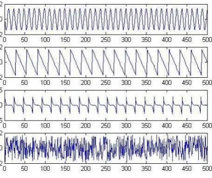
Figure 1. The source signals used in simulation.
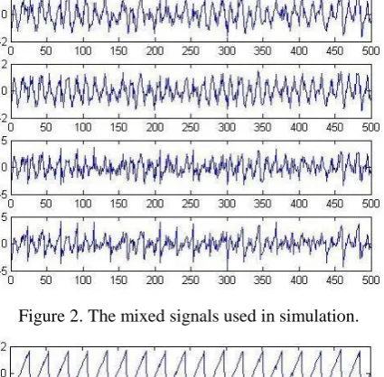
[image:4.595.193.406.388.597.2]A mixed matrix is generated randomly, and the matrix composed of four signal values is multiplied by the mixed matrix, that is, the source signal is physically transmitted through a transmission channel which response function is unknown. The results obtained are shown in Fig. 2. At this time, it is difficult to distinguish the characteristics of the original signal. The traditional ICA algorithm based on cumulants and KICA algorithm were used to calculate the randomly mixed signals, and the results obtained successfully separated the simulated source signals that participated in the verification calculation, as shown in Fig. 3 and Fig. 4.
[image:4.595.193.405.564.748.2]Figure 2. The mixed signals used in simulation.
Figure 4. The estimated signals separated by KICA.
Through simulation verification using simulated data, both traditional ICA algorithm and KICA algorithm can effectively separate all source signals from mixed signals. The results obtained by KICA separation are less affected by noise interference than those obtained by traditional ICA, and the results are more accurate. Although some signals are found to be flipped on the time domain feature in the processing result, and the order of each source signal is changed, this is caused by the principle of independent component analysis algorithm. At present, there is no effective method to solve this problem, but this phenomenon does not affect the estimated frequency domain feature of each source signal.
Summary
In this paper, based on the introduction of the basic principle and specific algorithm of KICA, the performance of traditional ICA and KICA are verified and compared quantitatively. The results show that KICA has better signal separation performance than the traditional ICA algorithm. After that, the algorithm is applied to the separation calculation of underwater vehicle navigation noise signal. After the simulation verification of simulation data, the signal of underwater vehicle vibration noise source is separated, and the feasibility and effectiveness of the algorithm are verified.
References
[1] S.J. Zhu, L. He. Vibration Control of Marine Machinery. National Defense Industry Press, Beijing, 2006.
[2] J.C. Ma, Y.L. Niu, H. Y. Chen. Blind Signal Processing. National Defense Industry Press, Beijing, 2006.
[3] F.R. Bach, M.I. Jordan. Kernel independent component analysis. Journal of Machine Learning Research, 3(2002) 1-48.
[4] G. Marc G. Classes of kernels for machine learning: a statistics perspective. Journal of Machine Learning Research, 2(2001) 299-312.
[5] B. Scholkopf, A.J. Smola. Learning with kernels. The MIT Press, Cambridge, 2001.
[6] S. Saitoh. Theory of reproducing kernels and its application. Longman Scientific & Technical, Harlow, 1988.