ENERGY EFFICIENT DISTRIBUTED IMAGE COMPRESSION USING JPEG2000 IN WIRELESS SENSOR NETWORKS (WSNS)

ERROR MODELING FOR STRUCTURAL DEFORMATIONS

OF MULTI-AXIS SYSTEM BASED ON SVR

ZHENZHONG LIU,LIANYU ZHAO, ZHI BIAN

School of Mechanical Engineer, Tianjin University of Technology, Tianjin 300384, China

ABSTRACT

Multi-axis system is constituted by the mechanical links, and the link position - load deformations are non-linear. That is an important factor to affect the positioning accuracy of multi-axis system. As the nonlinear characteristics of link position and load deformations, a novel method for modeling deformations of loaded components based on SVR was presented. The 2R manipulator load deformations error models were building by ε-support vector regression, and according to the model, the trajectory error compensation was simulated. The simulation of structure deformations models and motion error compensation of 2R manipulator shows the SVR method could be used to build the deformations error model effectively.

Keywords: Multi-axis System, Structural Deformation, SVR

1. INTRODUCTION

In manufacturing systems, the structural deformations caused by the stiffness are an important factor to affect the system positioning error. Multi-axis system is constituted by the mechanical linkage, and the link position - load deformations are non-linear. The link position - load deformations model would be difficult to be derived by simple measurement or mathematical methods.

The commonly used methods of structural deformations modeling are the direct method [1], the stiffness matrix method [2-4], the finite element method [5-7], the experimental method [8] and the synthesis method [9]. Li Bing [1] established the main stiffness model of variable axis CNC using the direct method. The method is simple, but the versatility is limited, only applicable to the stiffness modeling of the standard position and orientation. Based on influence coefficient method and principle of virtual work, Zhao Tieshi [2] established continuous stiffness nonlinear mapping general model of spatial parallel mechanism, including the elastic deformations of active and passive hinge and gravities factor. Combining the stiffness matrix, the performance index k’ used to estimate the mechanism stiffness is defined, but it cannot come to the exact solution. Deng Yaohua [5] studied prediction of flexible material deformations using spline finite element method. This method has a good calculation speed, but large error is existed with the practical engineering. Gosselin [8] through the static stiffness experiments solved the machine

static stiffness by the method of loading and measurement deformations. It is a way to objectively reflect the actual working conditions, but the experimental method is a larger workload. Clinton [9] assumed linear relationship between the stiffness and length. With the minimum average error as the optimization goal, the stiffness calculation model was obtained by 42 measurement data, but in fact the stiffness and length is often non-linear.

For the nonlinear relationship between the link position and its deflection of the nonlinear transmission mechanism of the multi-axis system, this paper proposed the load deformations error modeling method based on support vector regression [10], and established the link position and load deformations model with support vector regression algorithm.

2. CHARACTERISTICS OF POSITION AND

LOAD DEFORMATIONS

L E,A,I _W

P L

P E,A,I q=W/L

(a) (b)

Figure 1: Force Conditions Of Links

By the material mechanics, the longitudinal deformations of figure 1(a) under the action of the tension P and gravity W are as follows:

/ , / 2

a a

p q

Y =PL ΕΑ Y =WL ΕΑ

In the formula, Y_pa represents a P generated

under tensile deformations; Y_qa is the generated

tensile deformations under the action of the uniform load W ; E is the modulus of elasticity of the material.

The bending deformations of the link:

b 3 b 3

q

/ 3 , / 8

p

Y =PL ΕΙ Y =WL ΕΙ

Wherein, Y_pb is the bending deformations under

the action of the force P ; Y_qb is the bending

deformations under the action of the uniform load q; and Idenotes the moment of inertia.

By the formula (1) and (2), the link position and the link deformations are non-linear when the change in the angle of the link with respect to the horizontal plane. I.e., the deformations of these components and the load on which are not directly proportional. The issue of the machining and assembly of parts cannot be guaranteed the link load is in the center line, the link but also by the influence of the torsional load, in most cases. Therefore, the deformations of the link rod are not easily obtained by a direct calculation method, and by actual measurement to obtain the accurate amount of deformations.

3. THE SUPPORT VECTOR REGRESSION

MODEL ALGORITHM

In this paper, ε-support vector regression builds the models of the deformations of the link rigidity, and its principles are as follows:

The sample data ( ,x y_{1 1}),, ( ,x yl l)∈(X×R) is

known. And ε-insensitive error loss function metrics of observed value y and function predictive value of f x( )= ⋅w φ( )x +b, that is:

0

( , ) max

( , )

i i

i i

y f x x

y f x x

ε _ε



− = _{ −}

−

 (3)

The slack variable (*) * *

1 1

( , , , _l, _l)T

ξ = ξ ξ ξ ξ and

the penalty function C are introduced. Then, the support vector machine regression transforms into mathematical optimization problem:

* * , , , 1 * * 1

min ( ) ( )

2 ( ( ) ) , . . ( ( ) ) , , 0 i i l i i w b i

i i i

i i i

i i

w w C

w x b y

s t y w x b

ε ξ ξ ξ

φ ε ξ

φ ε ξ

ξ ξ =  _{⋅ + +}    _{⋅ + − ≤ +}   _{− ⋅ + ≤ +}   ≥ 

∑

Introducing Lagrange function,

(*) (*) (*) * 1 * * 1 1 * 1 1 ( , , , , ) ( ) ( ) 2 ( ) ( ( ) ) ( ( ) ) l i i i l l

i i i i i i i i

i i

l

i i i i

i

L w b w w C

y w x b

y w x b

ξ α η ξ ξ

η ξ η ξ α ε ξ φ

α ε ξ φ

= = = = = ⋅ + + − + − + + − ⋅ − − + − + ⋅ +

∑

∑

∑

∑

Wherein, (*) * *

1 1

( , , , , )T l l

α = α α α α and

(*) * *

1 1

( , , , _l, _l)T

η = η η η η are Lagrange multiplier vectors. According to Fermat theorem,

* 1 * 1 (*) (*) (*) (*) (*)

( ) ( ) 0

( ) 0

0

0, 0

l

i i i

i l i i i i i i i i L w x w L b L C

α α φ

α α η α ξ α η = = ∂ _{= − − =} ∂ ∂ = − = ∂ ∂ = − − = ∂ ≥ ≥

∑

∑

Then, the dual form of optimization problem (4) is * * , ₁ * * 1 1 * * 1

min [ ( ) ( )]

1

( )( ) ( , ) 2

. . ( ) 0, 0 , / , 1, ,

l

i i i i

i

l l

i i j i i j

i j

l

i i i i

i

y y

K x x

s t C l i l

α α α ε α ε

α α α α

α α α α

In the formula, ( ,K x x_{i j})=φ( )x_i ⋅φ(x_j) is the kernel function. The original problem is transformed into the convex quadratic programming of the equation (7), and the solution

is *

( ,α α ), thus the regression equation:

*

( ) ( ) ( ) ( ,_{i j})

SV

f x = ⋅w φ x + =b

∑

*

* *

( ) ( , ) , (0, / )

( ) ( , ) , _i (0, / )

i i j i

j

k i k

j

b y K x x C l

b y K x x C l

α α ε α

α α ε α

= − − + ∈

= − − − ∈

∑

∑

4. THE ESTABLISHMENT OF THE

TRAINING SAMPLES

This paper describes the stiffness deformations modeling method based on SVR, with 2R manipulator as the research object shown in Figure 2.

A Z

X m 1

2

X1

l

l

m

θ1

θ2 B

P

Figure 2: The Force Conditions Of The 2R Manipulator Link

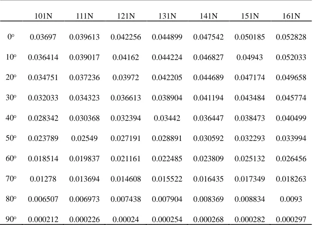
The DH parameters of the two links of the 2R manipulator are consistent. The links are hollow pipes. The length of the two links is 600mm. The inner circle of the two links is 60mm. The OD of the two links is 80mm, and the material of the two links is 45 # steel. The load deformations are analyzed by the finite element software Ansys to obtain the sample data. Make link1 and link2 of 2R manipulator respectively with the Cartesian coordinates X axis from 0° to 90°. The end (link2) of 2R manipulator is applied from 0N to 60N with load P. The load direction of the links is perpendicular to the X axis. Considering influence of its own gravity, the load range of the link 2 at the joints B is from 101N to 161N. The load deformations of link1 and link2 are analyzed, as shown in table 1 and table 2.

Table 1: Deformations Analysis Results Of Link1 (Unit: Mm)

101N 111N 121N 131N 141N 151N 161N

Table 2: Deformations Analysis Results Of Link2 (Unit: Mm)

0 N 10 N 20 N 30 N 40 N 50 N 60 N

0° 0.009617 0.012158 0.014699 0.01724 0.019782 0.022322 0.024863 10° 0.009471 0.011974 0.014477 0.01698 0.019483 0.021985 0.024489 20° 0.009039 0.011427 0.013816 0.016204 0.018593 0.02098 0.02337 30° 0.008331 0.010533 0.012734 0.014936 0.017137 0.019338 0.02154 40° 0.00737 0.009318 0.011266 0.013213 0.015161 0.017108 0.019057 50° 0.006186 0.007821 0.009455 0.01109 0.012725 0.014358 0.015994 60° 0.004813 0.006085 0.007357 0.008629 0.009901 0.011173 0.012445 70° 0.003295 0.004166 0.005036 0.005907 0.006777 0.007648 0.008519 80° 0.001677 0.00212 0.002562 0.003005 0.003448 0.003891 0.004334 90° 6.51E-05 7.82E-05 9.13E-05 1.04E-04 1.17E-04 1.31E-04 1.44E-04

5. TRAIN AND TEST OF THE STRUCTURE

DEFORMATIONS MODELS BASED ON SVR

Based on support vector regression algorithm, the samples were trained by the libSVM toolbox [11]. The kernel functionK x x( ,_{i j}) was elected the RBF kernel function:

2

2

( , ) exp 2

i i

x x K x x

σ

 ₋ 

 

= −

 

 

(10)

By experience method, the punishment factor C is 50, and the RBF kernel function width σ is 4. The table 1 and table 2 are the learning samples of error model, and the learning samples are as the test sample. The fitting results are as shown in table 3 and table 4.

Table 3: The Fitting Values Of Link1 Based On SVR (Unit: Mm)

101N 111N 121N 131N 141N 151N 161N

Table 4: The Fitting Values Of Link2 Based On SVR (Unit: Mm)

0 N 10 N 20 N 30 N 40 N 50 N 60 N

0° 0.009617 0.012158 0.014699 0.01724 0.019782 0.022322 0.024863 10° 0.009471 0.011974 0.014477 0.01698 0.019483 0.021985 0.024489 20° 0.009039 0.011427 0.013816 0.016204 0.018593 0.02098 0.02337 30° 0.008331 0.010533 0.012734 0.014936 0.017137 0.019338 0.02154 40° 0.00737 0.009318 0.011266 0.013213 0.015161 0.017108 0.019057 50° 0.006186 0.007821 0.009455 0.01109 0.012725 0.014358 0.015994 60° 0.004813 0.006085 0.007357 0.008629 0.009901 0.011173 0.012445 70° 0.003295 0.004166 0.005036 0.005907 0.006777 0.007648 0.008519 80° 0.001677 0.00212 0.002562 0.003005 0.003448 0.003891 0.004334 90° 6.51E-05 7.82E-05 9.13E-05 1.04E-04 1.17E-04 1.31E-04 1.44E-04

Compare table 1 and table 2 with table 3 and table 4, we can get: the errors between the fitting values by SVR and the Ansys simulation values are very small, which can be neglected. The SVR has

excellent function approximation ability. The fitting values of link2 by the least square method are as shown in table 5.

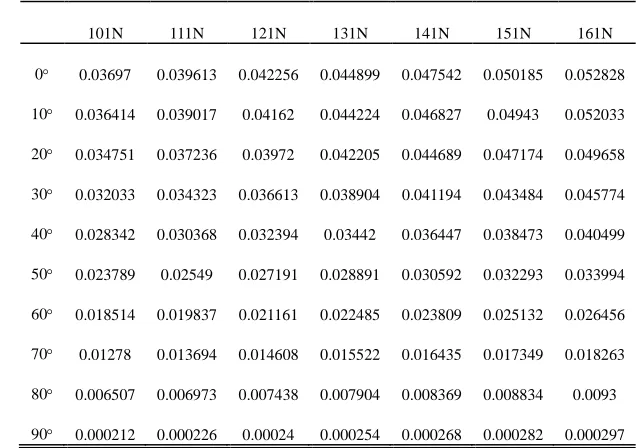
Table 5: The Fitting Values Of Link2 By The Least Square Method (Unit: Mm)

0 N 10 N 20 N 30 N 40 N 50 N 60 N

0° 0.009601 0.012138 0.014675 0.017212 0.019750 0.022286 0.024823 10° 0.009490 0.011998 0.014505 0.017013 0.019521 0.022027 0.024535 20° 0.009054 0.011446 0.013839 0.016231 0.018623 0.021014 0.023408 30° 0.008330 0.010531 0.012733 0.014934 0.017135 0.019335 0.021538 40° 0.007356 0.009300 0.011244 0.013188 0.015132 0.017075 0.019020 50° 0.006169 0.007800 0.009430 0.011061 0.012691 0.014321 0.015952 60° 0.004806 0.006077 0.007347 0.008618 0.009889 0.011159 0.012430 70° 0.003307 0.004181 0.005054 0.005927 0.006801 0.007675 0.008549 80° 0.001707 0.002157 0.002606 0.003056 0.003505 0.003955 0.004405 90° 4.46E-05 5.29E-05 6.11E-05 6.91E-05 7.73E-05 8.65E-05 9.48E-05

Contrast table 4 and table 5, we can obtain the errors are bigger by the least square method, and they are between 10 µm to 20 µm.

6. SIMULATION OF TEST SYSTEM

6.1 System Components

1 1 2

1 1 2

cos cos( )

sin sin( )

X l l

Z l l

θ θ θ

θ θ θ

= ⋅ + ⋅ +

= ⋅ + ⋅ + (11)

The invers kinematics are:

2 2 2

2

1 2 2

arccos( ( ) / 2 1)

arctan( / ) arctan( sin /( cos ))

X Z l

Z X l l l

θ π

θ θ θ

= − − + +

= − ⋅ + ⋅

(12)

6.2 Verification of the Structural Deformations Model

6.2.1 Experimental scheme

2R robot trajectories run for some distance along the Z-axis direction. The structural deformations errors of each link in the trajectory are analyzed based on SVR. Thus compensate for the error, and verify the validity of the structural deformation error model support vector regression analysis.

6.2.2 Experimental procedure

Let 2R manipulator trajectory run in the Cartesian coordinate, as [820, 0, 600] to [820, 0, 800] (unit: mm) of the straight line segments. Without considering the stiffness deformations, the angles of θ₁ and θ₂ are shown in Figure 3 and Figure 4.

600 620 640 660 680 700 720 740 760 780 800 0

5 10 15 20 25 30

The end Z-axis coordinate (mm)

The angular displacement of link

1

(°

)

Figure 3: θ₁ Angle Curve

The end Z-axis coordinate (mm)

The angular displacement of link

2

(°

)

600 620 640 660 680 700 720 740 760 780 800 30

35 40 45 50 55 60 65

Figure 4: θ₂ Angle Curve

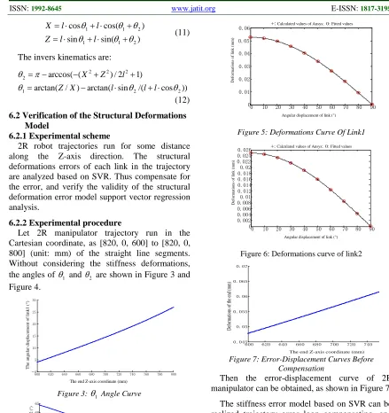
Assuming that the end load of the 2R robot is 60N, based on the aforementioned SVR modeling method, we can get the error models of link1 and link2 as shown in figure 5 and figure 6. The abscissa represents the angle of the link with the X axis, the ordinate is the amount of elastic deformations.

Deformations of link

(mm

)

+: Calculated values of Ansys; O:Fitted values

Angular displacement of link (°)

0 10 20 30 40 50 60 70 80 90

0 0.01 0.02 0.03 0.04 0.05 0.06

Figure5: Deformations Curve Of Link1

Deformations of link

(mm

)

+: Calculated values of Ansys; O:Fitted values

Angular displacement of link (°)

0 10 20 30 40 50 60 70 80 90

0 0.002 0.004 0.006 0.0080.01 0.012 0.014 0.016 0.018 0.02 0.022 0.024 0.026

Figure 6: Deformations curve of link2

The end Z-axis coordinate (mm)

Deformations of the end

(mm

)

600 620 640 660 680 700 720 740 0.045

0.05 0.055 0.06 0.065 0.07

Figure 7: Error-Displacement Curves Before

Compensation

Then the error-displacement curve of 2R manipulator can be obtained, as shown in Figure 7.

Trajectory discretization

Inverse kinematics

Error modeling based on SVR

Z = Z +ΔZ

Increments of each joint

ΔZ≤Δ

No

Yes

2R manipulator

Figure 8: The Algorithm Flowchart Of Error Loop Compensating

The end Z-axis coordinate (mm)

Deformations of the end

(mm

)

600 620 640 660 680 700 720 740 760 780 800 -1

-0.8 -0.6 -0.4 -0.2 0 0.2 0.4 0.6 0.8

1 x 10-3

Figure 9: Error-Displacement Curve After Compensation

Figure 8 show that the structural deformations have a large impact on multiaxial nonlinear link positioning accuracy. The structural deformations must be compensated. Figure 9 shows that the SVR can be effective used to the structure error compensation for multi-axis system. The structural deformation of the closed-loop error compensation can be achieved.

7. CONCLUSION

The structural deformations have a large impact on multiaxial nonlinear link positioning accuracy, and the structural deformations should be compensated. The SVR has excellent function approximation ability. It is better than the least square method. The simulation of structural deformations models and motion compensation of 2R manipulator shows the SVR method could be

effective used to build the structure error compensation for multi-axis system.

ACKNOWLEDGEMENTS

This work was supported by Tianjin Science and Technology Development Fund Project for Colleges and Universities under Grant No. 20120402.

REFERENCES:

[1] Li Bing, Wang Zhixing, Hu Ying, “The stiffness calculation model of the new typed parallel machine tool”, Journal of Machine Design, Vol. 3, No. 3, 1993, pp. 14-16.

[2] Zhao Tieshi, Zhao Yanzhi, Bian Hui, et al, “Continuous stiffness nonlinear mapping of spatial parallel mechanism”, Chinese Journal of Mechanical Engineering, Vol. 44, No. 8, 2008, pp. 20-25.

[3] Wang Youyu, Huang Tian, Chetwynd D G, et al, “Analytical method for stiffness modeling of the tricept robot”, Chinese Journal of Mechanical Engineering, Vol. 44, No. 8, 2008, pp. 13-18.

[4] Anatoly Pashkevich, Damien Chablat, Philippe Wenger, “Stiffness analysis of overconstrained parallel manipulators”, Journal of Mechanism and Machine Theory, Vol. 44, No. 5, 2009, pp. 966-982.

[5] Deng Yaohua, Liu Guixiong, Wu Liming, et al, “Deformation prediction of flexible workpieces and an error compensation method in NC machining processing”, Mechanical Science and Technology for Aerospace Engineering, Vol. 29, No. 7, 2010, pp. 846-851.

[6] Peng Zhi, Wang Lipeng, Wang Xinyan, “The FEM analysis for guideway deformation advance compensation of CNC machine tool”, Machine Tools & Hydraulics, Vol. 39, No. 12, 2011, pp. 26-27.

[7] Bashar S. E., PLACID M. F., “Computation of stiffness and stiffness bounds for parallel link manipulators”, International Journal of Machine Tools & Manufacture, Vol. 39, No. 2, 1999, pp. 321-342.

[9] Charles M Clinton, Guangming Zhang, “Stiffness moding of a stewart-platform-based milling machine”, Trans of the North America Manufacturing Research Institution of SME, No. 25, 1997, pp. 335-340.

[10] Chapelle O, “Choosing multiple parameter for support vector machines”, Machine Learning, Vol. 46, No. 1, 2002, pp. 131-159.