WRL TN 62 pdf

(1)

Fay Chang

Keith Farkas

Parthasarathy Ranganathan

(2)

The Western Research Laboratory (WRL), located in Palo Alto, California, is part of Compaq’s Corporate Research group. WRL was founded by Digital Equipment Corporation in 1982. We focus on information tech-nology that is relevant to the technical strategy of the Corporation, and that has the potential to open new business opportunities. Research at WRL includes Internet protocol design and implementation, tools to optimize com-piled binary code files, hardware and software mechanisms to support scalable shared memory, graphics VLSI ICs, handheld computing, and more. As part of WRL tradition, we test our ideas by extensive software or hard-ware prototyping.

We publish the results of our work in a variety of journals, conferences, research reports, and technical notes. This document is a technical note. We use technical notes for rapid distribution of technical material; usually this represents research in progress. Research reports are normally accounts of completed research and may include material from earlier technical notes, conference papers, or magazine articles.

You can retrieve research reports and technical notes via the World Wide Web at: http://www.research.compaq.com/wrl/

(3)

Experiences with the iPAQ Pocket PC

Fay Chang, Keith Farkas, and Parthasarathy Ranganathan

Palo Alto Research Laboratories

Compaq Computer Corporation

fFay.Chang, Keith.Farkas, Parthasarathy [email protected]

1 Introduction

Energy is a critical resource for many computing systems, spurring the desire for energy-efficient software. To build such software, developers need to understand the energy impact of their software design decisions. Currently, when developers reason about such decisions, they tend to rely on intu-ition. However, intuition can be misleading because most developers do not internalize an accurate model of the energy cost of different operations, or properly account for the relative frequency of the operations that take place.

In this report, we describe a tool that can help developers quickly determine the energy impact of their design decisions. In particular, using our tool, a developer can quickly obtain a wealth of information about the system' s power and energy consumption while executing some software. For example, our tool can provide answers to questions like:

1. How does power consumption vary while executing the software?

2. What power states are exercised while executing the software, and how much energy is con-sumed in each of these power states?

3. Of the energy that is consumed, how much is consumed while executing each individual in-struction, procedure, and application?

Our tool is based on statistical sampling. Statistical sampling tools introduce a periodic source of interrupts. Whenever such an interrupt is received by the system, the tool records a samplethat contains information about the system' s state, such as a timestamp and the program counter of the interrupted instruction. The samples gathered during a given time period can then be analyzed to produce estimates of the system' s behavior during that time period.

(4)

The samples collected during energy-driven statistical sampling can be analyzed in a variety of ways. First, the average power consumed by the system during some time period is equal to the product of the energy quanta and the interrupt frequency during that period. Using this relationship, we can extract information about the system' s power consumption. Second, the amount of energy consumed while executing some software is estimated by the product of the energy quanta and the number of samples that are attributed to that software. Consequently, we can extract information about the system' s energy consumption from the distribution of samples, i.e. theenergy profile.

In this report, we illustrate the type of information that can be obtained from our tool using a prototype we built of the tool for an iPAQ handheld running PocketPC. We begin in the next section by comparing our tool to other approaches for obtaining this information. Then,we describe our prototype implementation with Section 3 covering the hardware and Section 4 the software. Results are then presented in Section 6 for an energy-consumption study of 14 benchmarks. Finally, we summarize our findings in Section 7, and present an analysis of the errors in our approach in Section A.

2 Other Tools

Energy-driven statistical sampling can be used to measure average power consumption and to obtain temporal profiles or histograms of power consumption. It can also be used to measure total energy consumption and extract energy profiles that attribute that energy consumption to the software ex-ecuted during the sampling period. While there are other tools that can provide such information, we believe our tool offers several advantages.

First, a computer system' s power usage could also be characterized using measurement equipment like digital meters or data acquisition systems. However, the accuracy provided by such measurement equipment would often be excessive, so that our tool is a better option owing to its much lower hardware cost and greater ease of use.

Second, there are several other tools that seek to assist developers in mapping energy consumption to software components. Most of these tools estimate energy consumption by multiplying activation counts for various activities (e.g. executing a particular type of instruction) with estimates of the en-ergy consumed to perform each activity [2, 4, 9]. One advantage of this approach is that it can leverage activation counts for background activities to more easily attribute energy consumed asynchronously. However, an activation-based approach has the disadvantage of requiring system-specific knowledge about what activities should be counted, and system-specific estimates of the energy consumed to perform each such activity.

(5)

current-sense amplifier

monostable multivibrator

12-bit binary counter

Q

Energy Counter iPAQ H36xx

processor (SA 1110)

gpio battery terminals Bench

Power Supply

i_s

i_m Vs

C

Vb

[image:5.612.149.456.109.233.2]

Vx

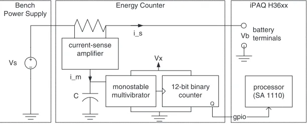
Figure 1: Block diagram of the iPAQ-based energy-driven sampling prototypes. The energy counter is interposed between the power supply and the iPAQ handheld computer.

3 Hardware

In this section, we describe our hardware implementation of the energy-counter and the two iPAQ-based prototype systems that use it. Both of our prototypes are iPAQ-based on iPAQ units that had their Flash ROM capacity upgraded from 16 MB to 32 MB. Unit 1 is a production H3630 unit, while unit 2 is a pre-production H3600 unit.

3.1 Hardware Overview

Figure 1 presents a block diagram of our two prototypes. As shown, we replaced the battery of the iPAQ handheld with a power supply, and interposed an energy counter between the power supply and the iPAQ' s electronics. We used a power supply rather than the battery to simplify our experi-mental procedure and to ensure that the iPAQ' s power efficiency stays constant during experiments; Section A.1.1 discusses the consequences of using a battery. The purpose of the energy counter is to generate an interrupt whenever a predetermined amount of energy has been consumed. The energy counter operates as follows.

As current

i

s

is drawn from the power supply by the iPAQ, a current mirror composed of a resistor and a current-sense amplifier generates a current

i

m

=

i

s

(the value of

is given in column 3 of

Table 1). This current

i

m

deposits charge on the positive plate of a capacitor, which acts as a current integrator. When the voltage across the capacitor plates reaches 2

3

of the voltage (

V

x

) powering the monostable multivibrator this IC generates an output pulse

P

, and discharges the capacitor to a voltage of

V

x

3

. The capacitor then begins to accumulate charge again via

i

m

.

Each pulse

P

indicates that the capacitor (with capacitance

)

dt

=

C

V

x

3

(6)

E

q

=

Z

t

0

v

b

(

t

)

i

s

(

t

)

dt

=

Q

i

Z

t

0

v

b

(

t

)

dt

=

Q

i

V

b

(2)

We refer to

E

q

as the minimum energy quanta. The minimum energy quanta in our prototypes is given in column 4 of Table 1.

Each pulse increments the value of a 12-bit binary counter. This counter allows the user to select the number of minimum energy quantas that must be consumed before an interrupt is generated. Specifically, if the iPAQ' s general purpose I/O line (GPIO) is connected to bit

q

of the counter, then an interrupt is generated once2

(

q

+1)

quantas of energy have been consumed. We refer to this quantity as theenergy quanta. The user must select the the value of

q

manually.

3.2 Hardware Implementation Details

One of our design goals was to support profiling of the energy consumed by applications that use an 802.11b wireless radio. To this end, we designed the energy counter so that it would measure the current drawn by an iPAQ handheld and a PCMCIA sleeve. Figure 2 presents a picture of one of the two nearly-identical prototypes. The wiring diagram of the prototypes is shown in Figure 3(a); for ease of comparison with the block diagram of Figure 1, we have reproduced Figure 1 here as Figure 3(b).

As illustrated in Figure 3(a), we have added the current mirror to theflex that is used to convey power to the iPAQ handheld, while the rest of the energy-counter functionality is implemented by the

energy-counter PCB. We also modified the PCMCIA sleeve so as to monitor its current consumption

and to interface the energy-counter PCB to the iPAQ handheld.

We have removed the battery from both the iPAQ handheld and the PCMCIA sleeve, and replaced each with a piece of flex that contains a battery connector at one end, and power leads at the other (

P

1 and

P

3 in Figure 3(a)). With the iPAQ handheld, we then inserted the sense resistor

R

in series

with the positive power lead (

P

3); Column 2 of Table 1 lists the value of the sense resistor for each

prototype. To avoid measuring the current dissipated as heat in the fuse, we located

R

downstream of the fuse. With the PCMCIA sleeve, we shorted its fuse, and connected the positive power lead (

P

3) to

Prototype Resistor

Minimum Energy Quanta (

E

q

)

1, upgraded H3630 unit 100

m

0.001 46

J

2, upgraded pre-production H3600 unit 120

m

0.0012 38

J

(7)

[image:7.612.229.375.111.321.2]

Figure 2: One of our two iPAQ prototypes showing the iPAQ handheld and PCMCIA sleeve, the energy-counter PCB, and the bench supply that powers all three.

MAX 4172

Rs+ Rs-V+

gnd

out P3

(+)

battery connector iPAQ H3xxx

battery flex

P1 (gnd)

4.1

PCMCIA sleeve battery flex (fuse removed)

P3 (+) P1

existing fuse

int_op (gpio 24)

pcm_vdd_on (U37 pin 8)

energy counter PCB current in interrupt enable

R Vdd gnd

(a) Wiring diagram

12-bit binary counter

Q

processor (SA 1110) gpio

battery terminals Bench

Power Supply

i_s

i_m Vs

C

Vb Vx

(b) Block diagram

[image:7.612.74.516.388.600.2]

(8)

LMC 555 cmos timer V+

gnd

out

thresh dischg

reset

trig gnd

V+ Q11 Q1 Q0

clr interrupt (select one)

current in

Vdd enable

5000pF (polystyrene) 1uF 10nF

10nF

100k

[image:8.612.151.460.108.284.2]

74VHC4040 binary counter

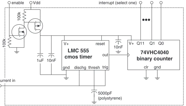
Figure 4: The energy-counter PCB.

the downstream end of the resistor

R

such that the current consumed by both the sleeve and the iPAQ handheld would flow through

R

.

To maximize the signal to noise ratio, we installed the current mirror (MAX 4172) adjacent to the sense resistor and connected its output to the energy-counter PCB. The energy-counter PCB (shown in Figure 4) contains the monostable multivibrator and the 12-bit binary counter.

The energy-counter PCB (Figure 4) is powered by the 3.3 V source (Vdd) generated by the iPAQ handheld and distributed to the sleeve. However, since the sleeve cannot draw more than 10 mA during sleeve initialization [5], two transistors disconnect the ICs from Vdd until a signal generated by the PCMCIA sleeve (pcm vdd on) is asserted. The 5000 pF capacitor integrates the current generated by the current mirror and conveyed to the capacitor via the signalcurrent in. When the pre-determined amount of energy is consumed, the energy quanta, an interrupt request is signaled to the processor viaint op(GPIO 24). The user must manually connect this signal to one of the outputs of the binary counter.

4 Software

In this section, we describe the software for energy-driven statistical sampling, and the simple exten-sion of this software that allows it to also support time-driven statistical sampling. The software runs within/on the Merlin build of PocketPC for the iPAQ.

4.1 Software Overview

(9)

modifications Other kernel

PID RAM executable

mappings sample buffer

64KB

Data-Sample data files buffered

sample info

Kernel device driver

program copy

copy Sampling

interrupt

ISR Sampling

Sampling

Enable/disable profiling

[image:9.612.103.501.110.216.2]

collection

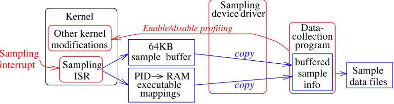
Figure 5: Data collection software

the addition of an interrupt service routine (ISR) for handling sampling interrupts, the reservation of memory buffers for holding sample data, and support for controlling (e.g. enabling and disabling) sampling via the device driver.

Figure 5 presents a block diagram of the data-collection software. A user enables and disables sampling via the user-level data-collection program (which issues calls to the device driver, which may in turn issue calls to the kernel). Sampling interrupts are generated only when sampling is enabled. When the kernel receives a sampling interrupt, it suspends the executable that was being executed and calls the added ISR. The ISR records a 16 B sample in a pre-allocated 64 KB RAM buffer, where each sample consists of:

PC – the program counter address of the interrupted instruction;

Module ID – a value that identifies the software module (executable or dynamically linked library) in which this instruction resides;

Executable ID – a value that identifies the interrupted executable (so that the interrupted executable can be identified even if the interrupted instruction resides in a DLL); and

Time stamp – the value in the operating system count register, which is incremented autonomously by the processor every271 ns.

Each executable and DLL stored in ROM is identified uniquely using its readily-available table-of-contents pointer. Unfortunately, there is no corresponding identifier for executables and DLLs stored in RAM. To enable efficient identification of RAM executables, the ISR maintains (in another pre-allocated RAM buffer) a mapping from the process identifiers of sampled RAM executables to their executable names. These process identifiers are used by the ISR as the Executable ID for the samples that belong to such executables. The software does not currently, but could easily be extended to, uniquely identify RAM DLLs as well. (We did not include this functionality because the percentage of samples in RAM DLLs was insignificant during all of our benchmarks.)

(10)

data files. Such data files can be processed using the data-processing tools at any subsequent time to produce various textual and graphical summaries of the sample data that was collected.

We have also extended the software to support time-driven sampling. In this mode, rather than using our energy counter to generate an aperiodic stream of sampling interrupts, we use one of the processor' s operating system timers to generate a periodic stream of sampling interrupts. Thus, our time-driven sampler does not require any additional hardware. The user-level data-collection program allows a user to enable either energy-driven or time-driven sampling. It also allows a user to set the sampling frequency for time-driven sampling.

4.2 Software Implementation Details

We found that attempting to write all of the sample data to the RAM-based file system while sampling is enabled noticeably disrupted the performance of the system, and therefore the samples that were collected. Two possible approaches for addressing this problem are: 1) to decrease the amount of data written by writing only a subset or a summary of the sample data, and 2) to buffer the sample data in RAM until sample collection is stopped. The first approach loses some information. Notice, however, that some of the information that can be extracted from the sample data may not be of interest to the particular user of the sampling system. For example, if a user of the sampling tool is interested in energy consumption, but not in power consumption, then the time stamps in the samples are superfluous. The amount of data saved could also be reduced by coalescing samples (e.g. by executable ID). In order to demonstrate the different types of information that could be extracted from the sample data recorded by the ISR, we currently use the second approach of buffering sample data until sample collection is stopped.

Table 2 summarizes the modifications and additions we made to the OEM Adaptation Layer (OAL) for the iPAQ.

5 Experimental Methodology

(11)

File Modification

kernel/hal/cfwzilker.c Added code to allow the sampling device driver to con-trol whether energy/time-driven sampling is enabled or disabled.

kernel/hal/arm/int1110.c Added interrupt service routine (ISR) that records a sample upon receiving a sampling interrupt.

drivers/eprof/* New sampling device driver (which exports a stream

in-terface).

drivers/dirs Added statement that causes the sampling device driver

to be built by the code generation tools.

inc/drv glob.h Added global variables shared by the sampling device

driver and the kernel.

inc/eprof.h New definitions shared by the sampling device driver

and the kernel.

inc/oalintr.h Added definition of an interrupt value for sampling.

files/config.bib Reserved a fixed 64 KB RAM buffer in which the

sampling ISR records samples.

files/eprofgui.exe New program via which users can control sampling.

While the source for this program was not added to the OAL, it was convenient to include the executable in the iPAQ PocketPC build.

files/platform.bib Added entries so that sampling device driver and

user-level program would be included in iPAQ PocketPC build.

files/platform.reg Added entries so that sampling device driver would be

[image:11.612.92.513.105.468.2]

included as a built-in driver.

Table 2: Modifications in the OAL to implement energy-driven and time-driven statistical sampling. We also modifiedint1110.c,cfwzilker.candtimer.cto fix the bug in the unmodified OAL code that caused all interrupts to be cleared while servicing any interrupt (rather than clearing only the serviced interrupt).

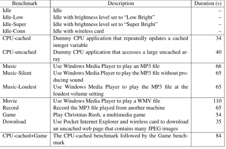
Sample Collection

(12)

notice-Benchmark Description Duration (s)

Idle Idle –

Idle-Low Idle with brightness level set to “Low Bright” – Idle-Super Idle with brightness level set to “Super Bright” –

Idle-Conn Idle with wireless card –

CPU-cached Dummy CPU application that repeatedly updates a cached integer variable

34

CPU-uncached Dummy CPU application that accesses a large uncached ar-ray

40

Music Use Windows Media Player to play an MP3 file 66 Music-Silent Use Windows Media Player to play the MP3 file without

pro-ducing sound

65

Music-Loudest Use Windows Media Player to play the MP3 file at the loudest volume setting

65

Movie Use Windows Media Player to play a WMV file 110 Record Record the MP3 file played from another machine 65

Game Play Christmas Rush, a multimedia game 54

Download Use Pocket Internet Explorer and wireless card to download an uncached web page that contains many JPEG images

35

CPU-cached+Game The CPU-cached benchmark followed by the Game bench-mark

[image:12.612.82.525.109.401.2]

84

Table 3: Benchmarks and their run time.

ably perturbing the collected sample data. For our benchmarks, they resulted in a maximum average data collection rate of approximately 8 KB/second, and a peak data collection rate of approximately 10 KB/second. During our benchmarks, new sample data is copied into the data-collection program' s user-level buffer (and the data-collection program is awakened) at most once every 1024 samples.

6 Results

(13)

Benchmark Ave sampling Ave power Number of % samples frequency (Hz) (mW) samples inOEMIdle

(1) (2) (3) (4)

Idle 93 273 – 98

Idle-Low 251 738 – 99

Idle-Super 417 1226 – 99

Idle-Conn 383 1126 – 99

CPU-cached 260 765 8192 7

CPU-uncached 381 1120 14336 14

Music 230 676 16384 45

Music-Silent 218 641 14216 44

Music-Loudest 256 753 16384 47

Movie 303 891 32768 19

Record 157 462 10196 74

Game 409 1202 21504 1

Download 535 1573 18932 18

[image:13.612.118.486.107.345.2]

CPU-cached+Game 348 1023 28672 3

Table 4: Average sampling frequency, corresponding average power consumption, number of samples, and percentage of samples attributed to theOEMIdleroutine for each of our benchmarks. Average power consumption is the product of average sample frequency and the energy quanta, 2.94 mJ.

6.1 Power consumption

Energy-driven statistical sampling can be used to measure and compare the base power consumption of the system in various modes (e.g. idle with the backlight powered at various intensities). Spe-cifically, the power consumption in some mode can be calculated as the product of the energy quanta and the average sampling frequency in that mode. Further the relative sampling frequency in two modes indicates the relative power consumption of those modes. Table 4 presents the average power consumption for our benchmarks.

Column 1 of the table shows the average sampling frequency during each of our benchmarks, while column 2 provides the corresponding average power consumption. Observe that, for example, idling with the backlight on at its lowest setting (Idle-Low) causes the unit to consume 2.7 times the power of idling with the backlight off (Idle). Alternatively, idling with the backlight off and the wire-less card inserted (Idle-Conn) causes the system to consume almost as much power as idling with the backlight on at its highest setting without the wireless card (Idle-Super). In contrast, changing the speaker volume at which an MP3 file is played from the lowest setting (Music-Silent) to the highest setting (Music-Loudest) offered by Windows Media Player increased the system' s power consumption by only 17%.

(14)

between the two samples is simply the energy quanta divided by the time since the last sample. There-fore, energy-driven statistical sampling can also provide temporal profiles and histograms of power consumption.

6.1.1 Temporal Power-Consumption Profiles

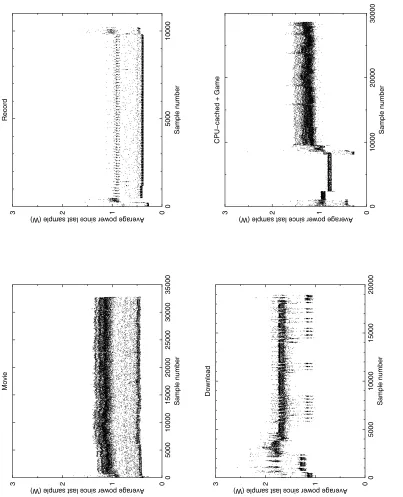
Figures 6 and 7 show temporal profiles of power consumption for a representative subset of our bench-marks. In each graph, the samples are ordered in time sequence along the x-axis, and the correspond-ing power consumption values are plotted on the y-axis. In order to show details that are obscured when data points are spaced very closely, Figure 6 includes a close-up of a portion of the temporal profile for theMusicbenchmark.

Spikes or shifts in temporal profiles can be correlated with events that occur during a bench-mark. For example, the noisy interval at the beginning and end of the temporal profiles of many of the benchmarks corresponds to touch screen navigation to start up and terminate the benchmark ap-plication, while the CPU-intensive benchmarks experience a downward shift in power consumption when the audio system times out and powers itself down1_{. In addition, the}_Download_benchmark

experiences downward spikes in power consumption which correspond to times during which the iPAQ is simply waiting to receive more data, while the shift from lower to higher power consump-tion during the sequentialCPU-cached + Gamebenchmark corresponds to the transition between runningCPU-cached and runningGame. The detail of the temporal profile for theMusic bench-mark reveals the granularity at which the CPU alternates between idle and busy times while playing an MP3 file. During most of the benchmarks, however, sampling intervals corresponding to lower and higher power consumption are interspersed very finely, indicating that those benchmarks do not contain distinct phases in which they operate at different power consumption levels.

The temporal profiles also reveal that, unsurprisingly, power varies the least for the benchmarks that contain the least amount of variation in activity (i.e. the idle and CPU-intensive benchmarks). The temporal profiles of all the other benchmarks show frequent incidence of power consumption at substantially different levels.

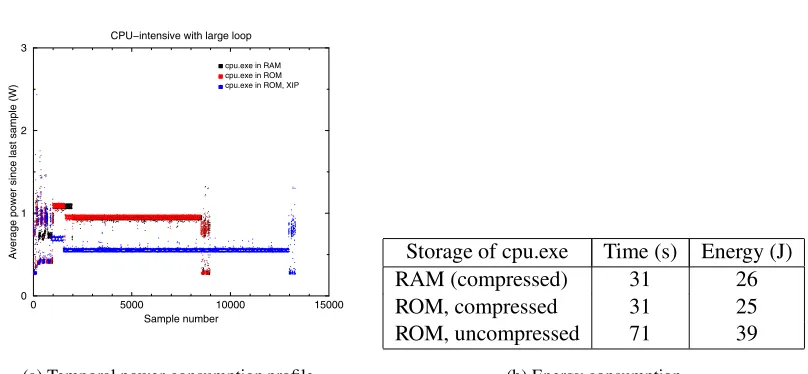
As another example of the insight that temporal profiles provide, we investigated how power and energy consumption change depending on whether a program is stored compressed in the RAM file system, compressed in ROM, or uncompressed in ROM. In the first two cases, the program is uncom-pressed and paged into RAM when executed; in the latter case, the program is executed directly out of ROM. We used two benchmarks: 1) executing a contrived CPU-intensive program which consists of a loop of simple arithmetic operations that does not fit in the processor' s instruction cache and 2) playing an MP3 file that is stored in RAM with Windows Media Player. For the execute-in-place case of the second benchmark, we use the default compression settings in the Merlin iPAQ build, which specify that the resources should be compressed in ROM (and therefore decompressed and copied into RAM before use).

For the uncacheable benchmark, Figure 8(a) shows the temporal power-consumption profiles, and Figure 8(b) shows total time and energy consumption, for all three cases. These results show

1_{The audio system is powered at the beginning of all the benchmarks except the idle benchmarks because the system}

(15)

1024 2048 3072 4096 Sample number 0 1 2

3 _{Average power since last sample (W)}

Idle

Idle−Super Idle−Conn Idle−Low Idle

0 5000 10000 15000 Sample number 0 1 2

CPU − intensive CPU − uncached CPU − cached 0 5000 10000 15000 Sample number 0 1 2

Music 5000 5250 5500 5750 6000 Sample number 0 1 2

[image:15.612.74.507.137.647.2]

(16)

0 5000 10000 15000 20000 25000 30000 35000 Sample number 0 1 2

Movie 0 5000 10000 Sample number 0 1 2

Record 0 5000 10000 15000 20000 Sample number 0 1 2

Download 0 10000 20000 30000 Sample number 0 1 2

CPU

−

cached + Game

[image:16.612.90.493.143.640.2]

(17)

0 5000 10000 15000 Sample number

0 1 2 3

Average power since last sample (W)

CPU−intensive with large loop

cpu.exe in RAM cpu.exe in ROM cpu.exe in ROM, XIP

(a) Temporal power-consumption profile

Storage of cpu.exe Time (s) Energy (J) RAM (compressed) 31 26 ROM, compressed 31 25 ROM, uncompressed 71 39

[image:17.612.108.512.110.297.2]

(b) Energy consumption

Figure 8: Impact on power and energy consumption of storing an executable compressed in either the RAM file system or ROM, so that it is uncompressed into and executed out of RAM, or storing it uncompressed in ROM so that it executes in place.

that, when executing out of ROM, this program takes much more time to complete, but consumes much less power. The decrease in power consumption is not sufficient to offset the increase in time, however, so that executing this program out of ROM consumes more energy. For the music playback benchmark, however, the average power, total time and total energy consumption are basically the same for all three cases. This reflects the fact that, relative to the prior benchmark, the instruction cache hit rate is much higher and instruction fetch is a much smaller component of the benchmark' s power consumption. From these results, it is clear that, for many applications, execute-in-place would save memory without increasing energy consumption. On the other hand, the slower access time of ROM could appreciably increase the latency and/or energy consumption of some applications that have high instruction cache miss rates.

6.1.2 Power-Consumption Histograms

Power-consumption histograms are useful for understanding the power levels during a benchmark. Figures 9 and 10 present power-consumption histograms for a representative subset of our bench-marks. In each histogram, the point (

x

,

y

) indicates that, for

y

% of the samples that were collected, the average power consumed by the system during the preceding inter-sample interval was

x

W. For clarity, the power values are grouped into 50 mW buckets.

(18)

0.0

0.5

1.0

1.5

2.0

0 20 40 60 80 100 % samples Idle CPU − cached CPU − uncached 0.0 0.5 1.0 1.5 2.0

0 10 20 30 % samples Music 0.0 0.5 1.0 1.5 2.0

0 10 20 % samples Movie 0.0 0.5 1.0 1.5 2.0

[image:18.612.74.492.146.656.2]

(19)

0.0

0.5

1.0

1.5

2.0

0

10

20

30

% samples

Game

0.0

0.5

1.0

1.5

2.0

0

10

20

30

40

% samples

Download

0.0

0.5

1.0

1.5

2.0

0

10

20

% samples

CPU

−

cached + Game

F

igur

e

10:

P

o

we

r-consum

ption

h

istogr

am

s

(fi

gur

e

2

of

[image:19.612.79.269.149.672.2]

(20)

However, the peak is wider, indicating that a range of power levels is exercised during the Game

benchmark. Finally, the histograms for all the other benchmarks show two significant peaks, indicat-ing that there are two significant power levels durindicat-ing each of these benchmarks.

The main power level during theCPU-cached andCPU-uncachedbenchmarks corresponds to the power consumption after the audio system timed out and powered down. The higher, secondary power level corresponds to the power consumption while the audio system was powered. The two peaks in the power-consumption histogram for the sequential CPU-cached + Game benchmark correspond to the peaks in the histograms of the individual benchmarks. Finally, to explicate the bi-modal nature of the remaining power-consumption histograms, Column 4 of Table 4 shows the percentage of samples attributed to theOEMIdle routine for each benchmark. For each benchmark, this percentage is an estimate of the percentage of energy that was consumed while the CPU was idling during that benchmark. Notice that the system tends to consume much less power when the CPU is idle than busy (as indicated by the power consumption figures in Column 2 of Table 4). Consequently, it is not surprising that there would be two separate peaks in the histogram of every benchmark that consumed a substantial percentage of energy while the CPU was idling as well as a substantial percentage of energy while the CPU was not idling. Moreover, it is not surprising that the lower peak should be less pronounced for the benchmarks that consumed a smaller percentage of energy while the CPU was idling.

Notice that the lower peak in each of the bi-modal histograms for the single-application bench-marks corresponds to a higher power level than the dominant power level during theIdlebenchmark. There are several possible reasons for this difference. One hypothesis is that the periods of time dur-ing which the CPU is busy are so finely interspersed with those durdur-ing which it is idle that the CPU will have been busy for some percentage of the time between any two samples. A second hypothesis is that, when the CPU is idle, thesystemis not necessarily idle, and the power consumed by such “asynchronous” system activity is responsible for the increased power level.

To investigate this latter hypothesis, we modified the OAL such that we could disable the audio system (by powering down the speaker and audio codec, and eliminating DMA to the audio subsys-tem) and/or the LCD subsystem (by eliminating LCD refresh and DMA to the LCD subsyssubsys-tem). We then experimented with disabling these subsystem while running the multimedia benchmarks. Our experiments validated this hypothesis. For example, Figure 11(a) shows power-consumption histo-grams for theMusicbenchmark when the audio subsystem was enabled or disabled. Disabling the audio subsystem shifted the power consumption histogram such that the lower mode is at the dominant power level of an idle system.

From Figure 11(a) we can also gain some insight into the characteristics of this asynchronous power consumption. In particular, note that the two peaks become more pronounced when the au-dio subsystem is disabled. This indicates that there was some variation in the asynchronous power consumption of the audio subsystem. This variation can obscure differences in synchronous power consumption. For example, Figure 11(b) shows power histograms for a game benchmark (that uses the same game as theGamebenchmark, but runs for a longer duration) when the audio and LCD sub-systems were either both enabled or both disabled. Notice that, with the audio and LCD subsub-systems disabled, the power histogram suggests a second, smaller peak at approximately 1.2 W.

(21)

sub-0.0 0.5 1.0 1.5 2.0 Average power since last sample (W)

0 10 20 30 40

% samples

Music

Audio system powered Audio system de−powered

0.0 0.5 1.0 1.5 2.0

Average power since last sample (W) 0

10 20 30

% samples

Game

[image:21.612.88.504.112.282.2]

Audio & LCD powered Audio & LCD de−powered

Figure 11: Power-consumption histograms for theMusicandGamebenchmarks with various sub-systems enabled or disabled.

system consumes about 120 mW when the system is idle. In other words, LCD refresh is responsible for 44% of the power that is consumed when the system is idle with the backlight off and the expansion pack empty.

6.2 Energy consumption

Energy-driven statistical sampling can also be used to develop insights into energy consumption. For example, the energy consumed to perform a task can be calculated as the product of the energy quanta and the number of samples recorded while performing that task. Further, the relative number of samples that are recorded while performing different tasks are indicative of their relative energy consumption. Column 3 of Table 4 shows the number of samples for each of the benchmarks that involved a particular task. From these figures, it can be seen that, for example, playing a particular MP3 file at the default volume consumed 1.6 times as much energy as recording that music (played from a separate system) with the default microphone settings.

Energy-driven statistical sampling can also be used to extract energy profiles that apportion the energy consumed to the software executed while the samples were collected. Specifically, since the rate at which sampling interrupts occur is proportional to the rate at which energy is being consumed, the percentage of samples attributed to some software is an estimate of the percentage of energy consumed while executing that software.

(22)

latter could be leveraged by users of a system to understand how they are using up the charge stored in the battery.

Given that energy-driven statistical sampling requires a small amount of hardware support that is not provided by most current systems, one question that warrants investigation is to what degree duration can serve as an approximation for energy consumption. To help answer this question, the rest of this section compares energy and time profiles.

6.2.1 Procedure-level Profiles

Figure 12 presents the procedure-level time and energy profiles for eight of our benchmarks. For each benchmark, the time and energy profiles individually identify all the procedures and modules to which 10% or more of the samples were attributed within either profile. All other procedures and modules are combined in “Other”. Procedures whose names were stripped from their binary are named as

UNKNOWN <starting address> <size>. Finally, the procedures and modules in each graph are ordered according to the number of samples that time profiling attributed to that procedure/module, so that it is easy to detect when energy profiling reveals a different ordering.

Time and energy profiles differ if the profiled workload exercises multiple, distinct power levels, which, as discussed in Section 6.1.2, is true for many of our benchmarks. For example, observe that, for the benchmarks that spend a lot of time with the CPU idle, the idle routine component of the time profile (i.e. OEMIdle) is much larger than the corresponding component of the energy profile. Similarly, the profiles forCPU-cached+Gameshow differences in the proportion of time and energy spent in the two executables. In particular, since time profiling is oblivious to the fact that Game

consumes energy at a much higher rate thanCPU-cached, time profiling greatly underestimates the relative energy consumption of playing the game.

If the profiled execution contains only a single dominant power level, however, time and energy profiles will not differ substantially. This is demonstrated by the similarity of the time and energy profiles for theGameandDownloadbenchmarks. It is also demonstrated by the similarity of the time and energy profiles of all of the benchmarks exceptCPU-cached+Gameif the samples attributed to

theOEMIdleroutine are ignored, as shown in Figure 13.

6.2.2 Discussion

The similarity in most of the profiles once the OEMIdle samples are ignored is an artifact of the current-generation iPAQ platform. In particular, with the exception of cache misses, all instruc-tions consume approximately the same amount of power [10]. The difference in power consump-tion due to cache misses is substantial, as illustrated by the histograms for the CPU-cached and

CPU-uncached benchmarks in Figure 9. However, most procedures include a mixture of instruc-tions and, as discussed in Section 6.1.2, the power consumed by background activity represents a noteworthy fraction of the overall power consumption. As a result, the higher power consumption of instructions that cause cache misses is usually not sufficient to create a substantial difference between time and energy profiles.

(23)

[image:23.612.98.506.118.650.2]

(24)

[image:24.612.98.507.119.653.2]

(25)

Module Time (%) Energy (%) App-206 22.01 41.13 App-59 77.44 57.50

Other 0.56 1.37

Module Time (%) Energy (%) App-59 31.36 20.52 App-89 20.84 17.56 App-118 15.67 16.32 App-148 12.47 15.57 App-176 10.33 14.92 App-206 8.85 14.56

[image:25.612.115.488.105.220.2]

Other 0.46 0.54

Table 5: Time and energy profiles that illustrate the impact of frequency scaling. This data was collected using our prototype built on top of an Itsy Pocket Computer.

time-driven statistical sampling can usually be used to approximate energy-driven statistical sampling by ignoring the samples attributed to theOEMIdleroutine. This conclusion, however, would not ne-cessarily apply to a system that offered the ability to dynamically and quickly change the speed at the which the processor runs. Such frequency changes would introduce other power states. Furthermore, future-generation processors that support voltage scaling in addition to frequency scaling are likely to display even greater variance in power states.

The impact that frequency and voltage scaling may have is suggested by the following two ex-periments. These two experiments were performed on a prototype we built using the Itsy Pocket Computer [3]. In the first experiment, we obtained time and energy profiles for a workload consisting of running a long benchmark twice, first at a clock frequency of 206 MHz, then at a clock frequency of 59 MHz. In the second experiment, we obtained time and energy profiles for a workload consist-ing of runnconsist-ing a short benchmark six times, each time with a different clock frequency (206 MHz, 176 MHz, 148 MHz, 118 MHz, 89 MHz and 59 MHz). Table 5 summarizes the results of these two experiments. While these workloads are synthetic, the results indicate the inappropriateness of time profiles for estimating the energy consumption of applications that exploit frequency scaling.

7 Summary and Future Work

While the issues with designing applications to reduce execution time are fairly well understood, a similar understanding of how to design applications to reduce their energy consumption is lacking. This report presented a new approach, energy-driven statistical sampling, that exposes information about energy consumption. Energy-driven statistical sampling tools can help developers both reason about the energy impact of software design decisions and identify application energy hot spots.

(26)

and the one we built for the Itsy pocket computer [3] indicate that energy-driven statistical sampling can provide an accurate system-level software energy profile with very little dynamic overhead or hardware cost.

For the iPAQ prototype, we have compared energy-driven statistical sampling to time-driven stat-istical sampling by comparing the profiles generated by these approaches for 14 benchmarks pro-grams. Our results show that there are often significant differences between the profiles generated by energy- and time-driven statistical sampling when the workload cycles through multiple power states. On simple handheld systems, such as current-generation iPAQ handhelds, many applications may exercise only a single power state other than idle mode. In such cases, time profiling should suffi-ciently approximate energy profiling for the purpose of assisting programmers. However, preliminary investigations indicate that emerging functionality, like frequency and voltage scaling, will increase the differences between time and energy profiles, and therefore the benefit of energy-driven statistical sampling.

A

Sources of Error

In this appendix, we discuss the sources of error in our energy-driving profiling approach. Broadly, the sources of error can be classified into two categories: (i) energy measurement related, and (ii) attribution and analysis related. The rest of this section discusses each of these in detail.

A.1 Measurement-related Errors

We begin our discussion of measurement-related errors with a discussion in Section A.1.1 of an error relating to battery-terminal voltage variation, and follow with a discussion of other errors in Sec-tion A.1.2.

A.1.1 Battery-terminal Voltage Variations

Energy-driven profiling operates on the assumption that each interrupt signifies that the iPAQ hand-held has consumed a fixed amount of energy. Since our energy counter integrates only the current being drawn by the iPAQ handheld, an equivalent assumption is that each interrupt signifies that a fixed amount of charge has been consumed. For an iPAQ handheld, the degree to which this latter assumption holds depends on the degree to which the battery-terminal voltage varies.

(27)

70 71 72 73 74 75 76 77

3.70 3.80 3.90 4.00 4.10 4.20 4.30

battery voltage mA 290 291 292 293 294 295 296 297 298 299 mW current power (current * voltage)

(a) Backlight off

370 375 380 385 390 395 400 405

3.70 3.80 3.90 4.00 4.10 4.20 4.30

battery voltage mA 1510 1520 1530 1540 1550 1560 1570 mW current power (current * voltage)

[image:27.612.102.500.119.276.2]

(b) Backlight full on and WL100 802.11b card

Figure 14: Current draw and power consumption as a function of supply voltage for iPAQ prototype #2 while the iPAQ was displaying the initial PocketPC “start” screen. (a) shows the relationship with the backlight off, while (b) shows the relationship with the backlight on at its highest setting and the WL100 802.11b card powered but with no driver loaded. Similar data was obtained with the other prototype and other scenarios.

The dependence on battery-terminal voltage can be ignored if (1) the battery-terminal voltage is held (essentially) constant, and (2) if the user of the profiler is interested only in comparing the relative energy cost of applications. If the first requirement is satisfied, then each interrupt will correspond to a fixed amount of energy. If the second requirement is true, then the user may safely ignored the exact value of the battery-terminal voltage since he/she does not need to know the value of the energy quanta. If, on the other hand, the user requires the value of the energy quanta, then an experiment, such as described in the caption of Table 1, must be done at each battery voltage of interest.

For our prototype, which uses a bench power supply, the battery-terminal voltage is sufficiently constant. The battery-terminal voltage is affected by two components: the regulation of the bench supply and the voltage drop across the fuse and sense resistor (see Figure 3(a)). The second component is the most significant since our bench supply is well-regulated. The impact of this component can be estimated by computing the relative increase in the number of samples attributed to a workload that occurs with decreasing battery voltage. This increase,

S

, is given by Equation 3, where

P

is the power the workload consumes at the nominal operating point,

P

is the change in power consumption due

to a decrease in battery voltage, while

I

and

I

are the comparable quantities for current.

S

=100

P

;

P

I

+

I

;1

(3)

(28)

preloadable count-down counter

zero

processor (SA 1110)

gpio battery terminals Bench

Power Supply

i_s

i_m Vs

C

Vb

Vx

[image:28.612.148.459.108.235.2]

new count

Figure 15: Block diagram showing in bold the components required to support software control of the energy quanta value.

we get

S

= 1.6%. This error is well within the margin of error of our approach.

If the iPAQ were powered by a battery rather than a bench supply, it may be important to explicitly account for the current-power relationship. One possibility would be to characterize the current-power relationship of the iPAQ, and then, using periodic sampling of the battery voltage, dynamically change the amount of energy that must be consumed before an interrupt is generated. Figure 15 illustrates how the basic energy-counter design can be modified to provide this functionality. As shown by the use of bold in the figure, we replace the 12-bit binary counter with a preloadable count-down counter, connect its zero-detect signal to one of the processor' s GPIOs, and map the counter into the memory space of the processor. The interrupt service routine used for profiling can then be modified so that, on servicing each interrupt, it writes a new count into the counter. Since this count is decremented each time the iPAQ consumes a minimum quanta of energy (see page 5), the software can change the amount of energy associated with an interrupt (the energy quanta) in steps equal to the minimum energy quanta.

A.1.2 Other Measurement-related Errors

A second measurement-related error is the inherent non-ideal characteristics of electrical compon-ents. Of particular note is the time required for the multivibrator to discharge the capacitor, which we determined empirically to be approximately 300 ns. For our benchmarks, the total time spent dur-ing such discharges of the capacitor represents a very small fraction of each benchmark' s run time. The other component-related errors are also negligible due to careful selection of components and operating ranges.

A third measurement-related error arises from the energy counter measuring the energy being consumed by some of the components (monostable vibrator and the binary counter, Figure 1) of which it is built. However, in practice, these components consume a negligible amount of energy compared to that consumed by the iPAQ.

(29)

energy profiling, and 0.13% or less for time profiling. Although the interrupt service routine cannot be profiled, we can measure the time spent in the routine. For time-driven sampling, the percentage of the total run time spent in the interrupt service routine is an estimate of the error it induces in the resulting time profiles. In our experiments, this percentage was 0.48% or less.

For energy-driven sampling, to estimate the error that the interrupt service routine induces in the resulting energy profiles, we first estimate the number of samples that would have been attributed to the routine, and then express this estimate as a percentage of the total number of samples. We estimate the number of samples that would have been attributed to the interrupt service handling routine by assuming that the average power consumption while executing the routine is approximately the same as during the initial portion of the CPU-uncached benchmark (i.e. before the audio system was powered down) since, as with the interrupt service routine, this benchmark is memory-intensive, does not include any idling, and does not use any devices. (We use the average power consumption while the audio system was powered because executing the interrupt service routine will not cause the audio system to be powered down if it is already powered.) For the Download benchmark, we adjust the assumed power consumption of the interrupt service routine by the increase in average power consumption due to the wireless card (i.e. the difference between the average power consumption of

IdleandIdle-Conn). Using this process, we estimate that the percentage of samples that would have been attributed to the interrupt sampling routine is 0.70% or less for all of our benchmarks. We have not estimated the error induced by calls to the sampling device driver because, with only the information currently recorded in each sample, the corresponding samples cannot be distinguished from samples due to other work performed by the device manager. However, experiments on the Itsy suggest that this error will also be very small.

A.2 Attribution Error

To accurately attribute a sample to an instruction, it is important to minimize the delay between the following two events: the monostable multivibrator generating a pulse

P

that will cause bit

q

of the binary counter to be asserted (see Section 3.1), and the interruption of the program in execution so that the interrupt can be serviced. This delay is composed of the time required for the interrupt to be conveyed to the processor core, and the time required for the processor to begin servicing the interrupt. For our prototype, the first component is on the order of nano-seconds, and is thus a small fraction of the time between interrupts, which is on the order of milliseconds. Given that the power consumed during such small time intervals does not vary significantly, the first component' s impact is a marginal variation in the energy quanta.

(30)

could be leveraged to adjust for this processor-induced skew in attribution.

A second source of error arises if phases of the application being profiled are synchronized ex-actly with the discharging of the capacitor. While we believe that this source of error is not likely to be exercised by applications, it may be guarded against by modifying the energy counter as suggested in Section A.1.1 to allow the value of the binary counter to be written by software. With this modi-fication, the energy quanta could be jittered by the interrupt service routine about some mean value. Our time-driven sampler trivially supports the ability to jitter its sampling frequency; in particular, during each interrupt, the time til the next sample was set to a random value within a small range such that the sampling frequency varied between 283 and 310 Hz during our Record and Download

benchmarks, and between 328 and 367 Hz during all of the other benchmarks.

Finally, a third source of error concerns sensitivity to the sampling rate. The accuracy with which a sample distribution reflects the true allocation of energy consumption for an application is proportional to the square root of the number of samples [6]. However, larger number of samples can lead to greater processing overhead and increased profiler intrusiveness. We performed sensitivity experiments in which we lowered the energy quanta to as little as 92

J, thereby increasing the number of samples by a factor of 32. We did not observe any significant difference in the procedure-level profiles.

References

[1] J. Anderson, L. Berc, J. Dean, S. Ghemawat, M. Henzinger, S. Leung, D. Sites, M. Vandevoorde, C. Waldspurger, and W. Weihl. Continuous profiling: where have all the cycles gone. In

Pro-ceedings of the 16th Symposium on Operating Systems Principles, October 1997.

[2] D. Brooks, V. Tiwari, and M. Martonosi. Wattch: A framework for architectural-level power analysis and optimizations. InProceedings of the 27th International Symposium on Computer

Architecture (ISCA), June 2000.

[3] Fay Chang, Keith I. Farkas, and Parthasarathy Ranganathan. Energy-driven statistical sampling: Detecting software hotspots. Technical Report WRL2002.1, Compaq Western Research Labor-atory, March 2002. This report is a reprint of a paper by the same title that appeared in the proceedings of the PACS 2002 workshop.

[4] T. L. Cignetti, K. Komarov, and C. Ellis. Energy estimation tools for the Palm. InProceedings

of the ACM MSWiM' 2000: Modeling, Analysis and Simulation of Wireless and Mobile Systems,

August 2000.

[5] Compaq. iPAQ H3000 series expansion pack developer guide, July 2000.

[6] J. Dean, J. E. Hicks, C. Waldspurger, B. Weihl, and George Chrysos. ProfileMe: Hardware support for instruction-level profiling on out-of-order processors. In Proceedings of the 30th

Annual International Symposium on Microarchitecture, December 1997.

[7] X. Zhang et al. Operating system support for automated profiling and optimization. In

(31)

[8] J. Flinn and M. Satyanarayanan. PowerScope: A tool for profiling the energy usage of mobile applications. InProceedings of the Workshop on Mobile Computing Systems and Applications

(WMCSA), pages 2–10, February 1999.

[9] J. Lorch and A. J. Smith. Energy consumption of Apple Macintosh computers. IEEE Micro

Magazine, 18(6), November/December 1998.