d i g i t a l
Automatic Motion Planning
for Complex Articulated Bodies
Publication Notes
This report is derived from lecture notes presented at the ACM SIGGRAPH’91 course C28:
Motion Synthesis, Planning, and Control, Las Vegas, Nevada, July 1991.
c
Digital Equipment Corporation 1992
This work may not be copied or reproduced in whole or in part for any commercial purpose. Permission to copy in whole or in part without payment of fee is granted for non-profit educational and research purposes provided that all such whole or partial copies include the following: a notice that such copying is by permission of the Paris Research Laboratory of Digital Equipment Centre Technique Europe, in Rueil-Malmaison, France; an acknowledgement of the authors and individual contributors to the work; and all applicable portions of the copyright notice. Copying, reproducing, or republishing for any other purpose shall require a license with payment of fee to the Paris Research Laboratory. All rights reserved.
Much research has been devoted to path planning during the past decade, i.e. the geometrical problem of finding a collision-free path between two given postures (configurations) of an articulated body (robot) among obstacles. This problem has straightforward applications in robotic automation, computer aided design, and computer graphics animation. Current global techniques compute explicitly the non-colliding zones in configuration space. Thus, they require exponential space and time in the number of Degrees of Freedom (DOF) of the body. These methods are therefore untractable for more than 4 DOF.
This report presents a new approach to path planning which does not require construction of an explicit description of the configuration space. The method consists of building and searching a graph connecting the local minima of a potential function defined over the configuration space. The graph is explored by means of a randomization technique that escapes the local minima by executing Brownian motions. This planner is considerably faster than previous path planners and it solves problems with many more degrees of freedom. Experiments are reported for several computer simulated robots, including rigid objects with 3 DOF (in 2D workspaces) and 6 DOF (in 3D workspaces) and articulated bodies with up to 30 DOF (in 2D and 3D workspaces).
R ´esum ´e
Le probl`eme de la planification de trajectoire consiste `a trouver des chemins sans collisions entre diff´erentes postures (configurations) d’un corps articul´e (robot), tout en ´evitant des obstacles d´efinis par un mod`ele g´eom´etrique. Des applications directes existent en robotique, en conception assit´ee par ordinateur, et en synth`ese de sc`enes graphiques anim´ees. Les techniques actuelles, dites globales, calculent explicitement toutes les postures autoris´ees du corps articul´e. Ainsi, elles n´ecessitent une espace m´emoire et un temps de calcul exponentiels en fonction du nombre de degr´es de libert´e (DDL) du corps. Ces m´ethodes sont donc inutilisables pour plus de 4 DDL.
Keywords
Path planning, motion synthesis, robotics, computer aided design, computer graphics, random-ization.
Acknowledgements
The results reported in these notes were obtained at the Computer Science Department, Stanford University, in collaboration with Prof. J.C. Latombe and B. Langlois. This research was funded by DARPA contract DAAA21-89-C0002 (Army), DARPA contract N00014-88-K-0620 (Office of Naval Research), SIMA (Stanford Institute of Manufacturing and Automation), CIFE (Stanford Center for Integrated Facility Engineering), and Digital Equipment Corporation’s external research program. We also benefited from discussions with Professor M. Harrison (Stanford Graduate School of Business) and J. Chang (Stanford Statistical Consulting Service)
2 Centralized versus Distributed Representations 4 2.1 Definitions : : : : : : : : : : : : : : : : : : : : : : : : : : : : : : : : : 4 2.2 Centralized Representations: the Problem of Collision Detection : : : 4 2.3 Distributed Representations : : : : : : : : : : : : : : : : : : : : : : : 5
3 Computation of Potential Field. 6
3.1 Overview : : : : : : : : : : : : : : : : : : : : : : : : : : : : : : : : : : 6 3.2 Workspace Potential Fields Without Local Minima : : : : : : : : : : : 6 3.3 Configuration Space Potential : : : : : : : : : : : : : : : : : : : : : : 8
4 Path Planning for Complex Articulated Bodies 9
4.1 Overview : : : : : : : : : : : : : : : : : : : : : : : : : : : : : : : : : : 9 4.2 Random Motions : : : : : : : : : : : : : : : : : : : : : : : : : : : : : : 10 4.3 Path Optimization : : : : : : : : : : : : : : : : : : : : : : : : : : : : : 12
5 Experimental Results 13
6 Discussion 18
7 Conclusion 19
1 Introduction
Much research has been devoted to robot motion planning during the past ten years (Latombe 1990 [26]). Most of this research has focused on path planning, i.e. the geometrical problem of finding a collision-free path between two given configurations of a robot. Today the mathematical and computational structures of the general problem (when stated in algebraic terms) are reasonably well understood (Schwartz and Sharir 1983 [37], Canny 1988 [10]). In addition, practical algorithms have been implemented in more or less specific cases (Brooks and Lozano-Perez 1983 [9], Gouzenes 1984 [20], Laugier and Germain 1985 [27], Faverjon 1986 [15], Lozano-Perez [31], Faverjon and Tournassoud 1987 [17], Barraquand Langlois and Latombe 1989a [4], Zhu and Latombe 1989 [39]).
One of the most widely studied path planning approach is the “cell decomposition” ap-proach (Brooks and Lozano-Perez 1983 [9]). It consists of first decomposing (exactly or approximately) the set of free configurations of the robot into a finite collection of cells and then searching a connectivity graph that represents the adjacency relation among these cells. However, in this approach, the number of cells to be generated is a function of the number of polynomial constraints used to model the robot and the obstacles, and of the degree of these constraints. This function also grows exponentially with the numbernof DOF’s of the robot,
as the volume of the configuration space increases exponentially withn. Thus, the approach
is intractable even for reasonably small values ofn. To our knowledge, no effective planner
has been implemented using this approach withn> 4. In fact, this is also true of the other
so-called “global” methods, e.g. retraction (ODunlaing Sharir and Yap 1983 [33]), which also represent the connectivity of free space in the form of a graph before actually starting the search for a path.
Some approximate cell decomposition methods proceed hierarchically by decomposing the configuration space into rectangular cells organized at several levels of resolution. For example, Faverjon[14] uses an “octree” to represent a three-dimensional configuration space. Each cell is labeled as EMPTY if it intersects no configuration space obstacle, FULL if it lies entirely in configuration space obstacles, and MIXED otherwise.
Since the intractability of the cell decomposition approach — and more generally of the other global path planning methods — is due to the precomputation of a connectivity graph representing the “global” topology of the robot’s free space, “local” methods to path planning have been developed for handling more DOF and some successful systems have been implemented, e.g. Donald 1984 [13], Faverjon and Tournassoud 1987 [17]. A local path planning method consists of searching the configuration space using heuristics computed from local geometric information. Thus, a local method requires no expensive precomputation step before starting the search of a path. In favorable cases, it runs substantially faster than any global method. But, since the search heuristics are only local, it may require much more time than global methods in less favorable cases, or even fail to find a path when one exists.
2 J ´er ˆome Barraquand
two components: a goal potential attracting the robot towards its goal configuration, and an obstacle potential, repulsing the robot from the obstacles. This so-called artificial potential
field approach was originally proposed in robotics as an on-line approach, applicable when the
robot does not have a prior model of the obstacles, but senses them during motion execution (Khatib 1986 [22]). Emphasis was put on real-time efficiency, rather than on completeness. In particular, since it acts as a gradient descent optimization procedure, this approach may get stuck at a local minimum of the potential function.
However, the idea underlying potential field can be combined with graph searching techniques to explore a grid placed over the robot’s configuration space. Then, if a prior model of the robot’s workspace is available, it can be turned into a systematic motion planning approach. This approach consists of incrementally building a graph connecting the local minima of the potential function defined over the robot’s configuration space and concurrently searching this graph until a goal configuration is attained. The local-minima graph plays a role similar to that of the connectivity graph in a cell decomposition approach (Brooks and Lozano-Perez 1983 [9], Schwartz and Sharir 1983 [37]). The major difference, however, is that it is constructed in an incremental fashion during the search. Hence, the approach does not require an expensive precomputation step. But local minima remain an important cause of inefficiency for planners based on such an approach. If there are too many of them, the planner may have to explore a large graph. Worse, if the attraction wells of the local minima are too large, the planner may spend much time finding a connection between two minima.
The local-minima problem can be addressed at two levels: (1) in the definition of the potential
function, by attempting to specify a function with no or few local minima; and (2) in the design of the search algorithm, by including appropriate techniques for escaping from local
minima. At the first level, the construction of analytical potentials free of local minima has been investigated, so far with limited success. Solutions have been proposed only in Euclidean configuration spaces with spherical or star-shaped obstacles (Koditschek 1987 [25], Rimon and Koditschek 1989 [36]). Another research has attempted to reduce the number of local minima and the size of their attraction wells by using superquadric potentials (Khosla and Volpe 1988 [24]). At the second level, there has been substantial research in the more general field of optimization and various methods have been proposed (e.g., simulated annealing (Kirkpatrick Gelatt and Vecchi 1983 [23])). But there has been no significant attempt to apply these results to motion planning.
The planning approach presented in these notes was originally proposed in Barraquand and Latombe 1989a [6]. It addresses the local-minima problem at the two levels mentioned above.
The principle of the method is the following:
1) construct goal-attractive potential fields over the workspace without spurious local minima,
each of them applying to a specific point of the robot.
2) combine these potentials into a configuration space potential implicitly defined by the
robot’s kinematics.
3) force the robot to remain in free space by checking that each new configuration explored is
collision-free. This corresponds in the classical potential field framework to assigning an obstacle-repulsive potential of zero in free space and infinity in colliding zones.
4) use a randomization technique to escape from local minima created by kinematic conflicts.
5) postprocess the resulting collision-free path to obtain smooth motions.
The method has been shown to be probabilistically complete, i.e. the probability to find a path if one exists tends toward 1 when the computation time tends toward infinity.
Experiments were conducted with the implemented planner using several computer-simulated robots, including rigid objects (“mobile robots”) with 3 DOF (in two-dimensional workspaces) and 6 DOF (in three-dimensional workspaces) and articulated objects (“manipulator arms”) with up to 31 DOF (in two- and three-dimensional workspaces). Some of the most significant experiments are reported in these notes. The planner demonstrated the following capabilities:
- It is much faster than any previous planner. For instance, a variant of this planner generates paths for a holonomic 3-DOF mobile robot in non-trivial workspaces in about 1 second of computation1, as opposed to minutes or even tens of minutes for most other planners. - It generates paths for robots with many DOF. In particular, within a few minutes of
computation, it constructs complex paths for a 10-DOF non-serial manipulator arm with both revolute and prismatic joints.
- It solves path planning problems for multiple robots. For example, without domain-specific heuristics, it can generate the coordinated paths of two 3-DOF mobile robots in a workspace made of narrow corridors.
Another advantage of the planner is that it accepts goals defined by specifying the desired positions of one or several points in the robot. This feature is essential when robots have many DOF, since specifying the goal configuration of the robot, i.e. a collision-free placement of the various bodies of the robot, is a difficult task in itself. It also allows easy handling of any kind of redundancy of the robot. Finally, a version of the planner (not described in this report) generates paths for nonholonomic robots. These are robots with non-integrable kinematic constraints such as a car and a car towing a trailer. This version of the planner is described in Barraquand and Latombe 1989b[7] and 1991[8].
This report is organized as follows. In Section 2, we discuss the representational issues for geometric primitives relevant to the path planning problem, and more specifically to the collision detection problem. In Section 3 we describe the construction of efficient attractive potential fields. In Section 4 we present the randomization method for escaping local minima of the potential field. In Section 5, we present experimental results illustrating the effectiveness of the approach proposed. Finally, in Section 6, we briefly discuss some theoretical and practical issues related to randomized planning.
1
4 J ´er ˆome Barraquand
2 Centralized versus Distributed Representations
2.1 Definitions
LetAdenote the robot,Wits workspace, andCits configuration space. A configuration of the
robot, i.e. a point inC, completely specifies the position of every point inAwith respect to a
coordinate system attached toW (Lozano-Perez 1983 [30]). Letnbe the dimension ofC, i.e.
the number of DOF. We represent a configurationq 2Cby a list ofnparameters (q1;:::;q
n
),with appropriate modulo arithmetic for the angular parameters (Latombe 1990 [26]). The subset ofCconsisting of all the configurations where the robot has no contact or intersection
with the obstacles inWis called the free space and is denoted byC
free
.For each pointp2A, one can consider the geometrical application that maps any configuration
q= (q1;:::;q
n
)2Cto the positionw2W ofpin the workspace. This map:X : AC ! W
(p;q) 7! X(p;q) =w
is called forward kinematic map.
2.2 Centralized Representations: the Problem of Collision Detection
Most solid modeling systems used in scientific computing or computer aided design represent geometric primitives by algebraic inequalities defining the boundaries of objects. This is also the case of systems used for the generation of computer graphics scenes. Often, the algebraic inequalities used are linear, and the geometric primitives are simply polyhedra. Representations of this kind are called centralized representations. The great advantage of centralized representations is that they provide a precise description of objects boundaries at any scale, while minimizing the amount of redundant information. Using such representations, accurate modeling of 3D structures can fit into the memory of current computer workstations. However, these representations have a severe drawback. They are unstructured, i.e. assessing the occupancy of a given location in space requires scanning the list of objects present in the scene. Therefore, detecting the collision of a given point in space with the objects present in the scene requires a time linear in the number of geometric primitives. Through the use of hierarchical representations such as octrees, the assessment of relative positions of static objects in the scene can be made much faster. Unfortunately, octree decompositions are not practical when some objects are movable, since they may change dramatically under small displacements.
The high computational requirements of automatic motion planning are mostly due to the need to perform repeated collision checking between the robot and the obstacles (Metivier and Urbschat 1990 [32]). Detecting the collision of a robot with many DOF in realistic environments may take as much as 1/10 to 1 second when using centralized representations. Automatic planning of a path requires a number of collision detections ranging from a few hundred for the simplest cases to a few hundreds of thousands for the most complex ones.
Such computation times are practically prohibitive for planning very complex motions using centralized representations.
An implementation of the planning approach reported here using centralized representations was tested in realistic industrial settings (Ohlund 1990 [34]). These experiments show that only relatively simple planning problems are computable in a reasonable amount of time with such representations. Fast hardware implementations of collision detection algorithms currently under development will hopefully circumvent these limitations (Libby 1990a [28] and 1990b [29], Cliff 1991 [12]). It may also be possible to improve collision detection algorithms for centralized representations using specific properties of the path planning problem, such as the continuity of the path (Faverjon 1991 [16]).
2.3 Distributed Representations
The experiments reported in these notes were all performed using a distributed representation of the workspace. The workspaceWis modeled as aN-dimensional bitmap array, withN = 2
or 3 being the dimension ofW. The array is defined by the following functionBM:
BM : W ! f1;0g x 7! BM(x)
in such a way that the subset of points x such that BM(x) = 1 represents the workspace
obstacles and the subset of pointsx such thatBM(x) = 0 represents the empty part of the
workspace. We write:W
empty
=fx j BM(x) = 0g.The main advantage of distributed representations is that they are structured, i.e. assessing the occupancy of any point in workspace is performed in a time constant in the number and shape of the obstacles, and in the resolution of the bitmap. A pointxis occupied if and only
ifBM(x) = 1. Consequently, checking the collision of the robot with obstacles can be done
by simply “drawing” the robot on the bitmap. The drawing procedures used are reminiscent of the Bresenham’s algorithm well known in Computer Graphics literature. Details on the collision detection methods employed can be found in (Barraquand and Latombe 1989a [6]). In the experiments reported in these notes, typical computation times for checking a collision with a complex robot ranged from 0.5 to 5 milliseconds on a DECstation 3100.
6 J ´er ˆome Barraquand
3 Computation of Potential Field.
3.1 Overview
The set of goal configurations of the robot is exogenously defined by a series of specific final positions for some particular points of the robot body. These particular points on the robot are called control points.
For each control pointp, a workspace potential field is computed in such a way that it has no
other local minimum than its desired final position. Such “perfect” potentials tends to keep the robot outside the workspace concavities created by the obstacles. When the workspace potentials are combined together – i.e., are applied concurrently to the different control points– the resulting configuration space potential may have (and indeed has) local minima other than the goal. However, it is usually possible to define the combination in such a way that either the number of minima or their domains of attraction remain small. The idea then is to build a graph connecting the local minima and perform a search of this graph until the goal is attained.
Let p1;:::;p
s
bes control points inA. For each point pi
we first construct the workspacepotential:
V
p
i :x2W
empty
7!Vp
i(x)2R
Then, using the forward kinematic mapX, we can combine the different workspace potentials
into another potential functionU defined over the configuration space:
U :q 2C
free
7!U(q) =G(Vp
1(X(p1;q));:::;V
p
s(X(p
s
;q)))2R:U is called the configuration space potential.
The construction of theV
p
i’s is described in the next subsection. The construction of U is
described in Subsection 3.3.
3.2 Workspace Potential Fields Without Local Minima
We want each functionV
p
ito have a single minimum at the goal position of the point
p
i
. Thisis a major heuristic step toward the construction of a configuration space potential with few or small spurious local minima.
In order to compute a workspace potential numerically, we need to construct of a triangulation ofW
empty
. By definition, a triangulation is a partition of the space in semi-algebraic convexcells such that any two adjacent cells share either a vertex or a face (edge in 2D). If the representation used is distributed, an obvious candidate for a triangulation of W
empty
isthe collection of free bitmap cells. If the representation is centralized, standard techniques derived from finite elements methods exist to compute such a triangulation (e.g. Delaunay
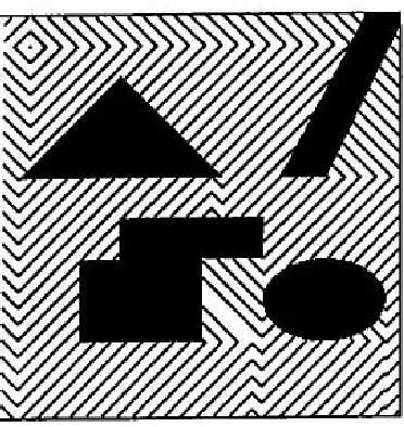
Figure 1: Equipotential Contours of the Workspace Potential.
triangulation). In the following, we will limit our presentation to the case of distributed representations without loss of generality.
The workspace potentialV
p
is computed for every control pointpusing a wavefront expansiontechnique starting at the goal positionx
goal
ofp. The value of Vp
is first set to 0 at xgoal
.Next, the value of V
p
at the neighbors of xgoal
in Wempty
is set to 1, the value of Vp
atthe neighbors of these neighbors in W
empty
is set to 2 (if not previously computed), etc.This procedure is recursively repeated until the connected subset ofW
empty
containingxgoal
has been completely explored. The complexity of this procedure is linear in the number of cells of the triangulation. When the representation is distributed, the number of such cells is upper bounded by the total number of bitmap cells. Then, the procedure becomes constant in the number and shape of the obstacles. Equipotential contours of the resulting workspace potential field for a two-dimensional workspace are displayed in Figure 1. This computation was performed in a fraction of a second.
Notice that V
p
is computed only in the connected subset of Wempty
that contains the goalpositionx
goal
. Hence, if the initial positionxinit
is not in the same connected component asthe goal, the value ofV
p
is not computed at this point, and we can immediately infer that thereis no collision-free path for the robot.
8 J ´er ˆome Barraquand
3.3 Configuration Space Potential
The goal configurations of a robot are specified by the goal positions of one or several points in the robot. By definition, the robot is at a goal configuration whenever all the control points are at their goal positions. For instance, ifAis a two-dimensional object that can both translate
and rotate in the plane (three-dimensional configuration space), the specification of the goal positions of two points uniquely determines the goal configuration of the robot. IfAis, say, a
10-DOF manipulator arm, specifying the desired positions of some points in the end-effector determines a goal region in configuration space.
It is important that a path planner allows one to specify a goal region in configuration space instead of a single goal configuration. Indeed, for many tasks, the goal configuration is incompletely specified. Arbitrarily selecting one would possibly result in a more difficult, or impossible, path planning problem. Furthermore, if the robot has many degrees of freedom, specifying a unique goal configuration is a difficult task in itself, since it requires a collision-free placement of the various bodies of the robot to be found.
The points used to specify the goal configurations of a robot are exactly those which are later used by the planner as the control points. Letp1;. . .;p
s
be these points. The configurationspace potentialU is defined as a combination:
U(q) =G(V
p
1(X(p1;q));. . .;V
p
s(X(p
s
;q)))of the workspace potentials V
p
i, i = 1;:::;s, defined for the s control points p
i
. Thiscombination concurrently attracts the different pointsp
i
toward their respective goal positions.The choice of the function G is important since it strongly influences the number of local
minima of the potentialU. With our “perfect” workspace potentials, the workspace concavities
do not directly create local minima. It is the concurrent attraction of the different control points toward their respective goal positions which creates these local minima. This results from the fact that these points do not move independently. As suggested above, the function
G precisely defines the way in which the competition between the different points is to be
regulated.
In most of the previous collision-avoidance systems using artificial potential fields,G was
chosen as a linear combination of the workspace potentials (Khatib 1986 [22]), i.e. :
G(y1;. . .;y
s
) =i
=s
X
i
=1i
yi
: (1)In the experiments reported here, non-linear expressions were used for the functionG, such
as:
G(y1;. . .;y
s
) =i
=s
max
i
=1y
i
: (2)This particular choice tends to increase the number of competitions between the control points and, therefore, the number of local minima. However, it can be a good choice for robots with many DOF. As a matter of fact, the number of local minima is not the only measure for the quality of the potential, since it might be much more difficult to escape a local minimum with a large attractive well than a minimum with a small well. The above competition functionG
increases the number of local minima, but experiments show that in general it also reduces their volumes. This is the function that gave the best results for planning the paths of manipulator arms with many DOF and multiple control points (see Section 5).
Unlike the workspace potentialsV
p
i, the configuration space potential
U does not have to be
precomputed before actually searching for a path. In fact, in high-dimensional configuration spaces, this precomputation would be untractable. The functionU is only computed during
the search of a path at those configurations which are attained by the search algorithm.
4 Path Planning for Complex Articulated Bodies
In this section we describe a version of the planner, called Randomized Path Planner (RPP), which has demonstrated its ability to solve many complex planning problems, some being non trivial for humans. When encountering a local minimum of the potential function, it applies a randomization procedure which consists of generating Brownian motions until the minimum is escaped. The resulting planning algorithm is probabilistically (rather than deterministically) resolution-complete. For robots with many DOF, the configuration space potential defined by formula (2) was used in the experiments, rather than the one defined by formula (1). However, the Monte-Carlo procedure itself does not depend on the particular potential function that is used.
4.1 Overview
Starting from the initial configurationq
init
of the robot, RPP first applies a best-first algorithm, i.e. it descends the potentialU, until it reaches a local minimumqloc
We call such a motion a gradient motion. LetUloc
=U(qloc
). IfUloc
= 0, the problem is solved and the planner returnsthe constructed path. Otherwise, it attempts to escape the local minimum by executing a series of random motions issued fromq
loc
. These random motions are approximations of Brownianmotions described in Subsection 4.2.
At the terminal configuration of every random motion, the algorithm executes a gradient motion until it reaches a new local minimum. The new local minimumq
new
with lowestpotential value is selected. IfU(q
new
)<U(qloc
), the same randomization procedure is appliedrecursively from q
new
. Else, if U(qnew
) U(qloc
), it is said that qloc
is a dead-end. In10 J ´er ˆome Barraquand
Thus, the graph of the local minima is incrementally built, the path joining two “adjacent” local minima being the concatenation of a random motion and a gradient motion. The randomized depth-first search outlined above is described in more detail in Barraquand and Latombe 1989a [6].
An interesting property of this planning algorithm is that all the random motions starting from a given local minimum can be performed concurrently on a parallel machine since there is no need for communication among the different processing units.
As the algorithm uses a random procedure to build the graph of the local minima, it is not guaranteed to find a path whenever one exists. In other words, the algorithm is not complete. However, the properties of Brownian motions make it possible to prove that when the number of Brownian motions executed from every local minimum is unbounded (the computation time may then tend toward infinity), the probability of reaching the goal converges toward 1. Hence, we say that the algorithm is probabilistically resolution-complete. However, this convergence-in-distribution property, which is well-known for the so-called “simulated annealing” algorithms (Geman and Hwang 1986 [19]), is a very weak one. Indeed, the totally uninformed algorithm which executes a Brownian motion from the initial configuration
q
init
and terminates when it enters a small neighborhood of the goal configuration, is alsoprobabilistically resolution-complete! Despite the weakness of this theoretical result, our experiments show that RPP is quite efficient.
We describe the generation of random motions in the following subsection. Further details can be found in Barraquand and Latombe 1989a [6].
4.2 Random Motions
When the algorithm reaches a local minimum of the potential fieldU, if no assumption is made on the statistics of the obstacle distribution, no additional information can be used for
reaching the goal. RPP continues the search by executing random motions issued from the current local minimumq
loc
.The most uninformed type of motion is known to be the Brownian motion (Papoulis 1965 [35]). Since a Brownian motion is a continuous stochastic process, the random motions performed by RPP are approximations of Brownian motions and are defined as discrete random walks. A random walk in the configuration space consists of executing a certain numbersof steps,
each step corresponding to a “time”∆t. The “duration” of the random walk ist= s∆t. Each
step projects into everyq
i
axis,i2[1;n], as an increment +∆i
or ∆i
of fixed amplitude, eachwith the constant probability 0.5 (hence, independent of the previous steps). The amplitude of the increment,∆
i
, is proportional to the “velocity” of the walk along theqi
axis. This randomwalk is known to converge almost surely toward a Brownian motion when the amplitude
∆
i
=vi
p∆tof every increment tends toward 0 as the square root of time (Papoulis 1965 [35]).
Without loss of generality, let us take the current local minimum,q
loc
, as the origin of thecoordinates ofC. The configuration attained by a Brownian motion of durationtand velocity
v
i
along each qi
axis is a random variable Q(t) = (Q1(t);. . .;Qn
(t)) with the followingfundamental property (Papoulis 1965 [35]):
The standard deviationD
i
(t) of the differenceQi
(t+t0) Qi
(t0) grows as the square root of t, i.e. :D
2
i
(t) = E(Q
i
(t0+t) Qi
(t0))2
= v
2
i
t:The Brownian motion (also called Wiener-Levy process) is well-defined as long as it does not encounter any obstacle in configuration space. When the processQ(t) hits the boundary
of an obstacle, the Brownian motion has to be adapted so that it remains in the free space. The classical generalization of a Brownian motion when the space is bounded consists of reflecting the motion that would have taken place in the absence of boundary, symmetrically to the tangent hyperplane of the boundary at the collision configuration (Brownian motion with “reflective boundary”). The mathematical consistency of this adaptation is discussed in detail in Anderson and Orey 1976 [1]. Our planner, which does not construct an explicit representation of the configuration space obstacles, does not know the orientation of the tangent hyperplane at the collision configuration. Hence, whenever a random motion step leads to collision with an obstacle, instead of reflecting the motion on the boundary, the planner guesses another random step and substitutes it for the previous one.
We still have to select the velocitiesv
i
and the durationtof every random motion. For the sakeof simplicity, we set∆t= 1. Since we approximate a Brownian motion as a random walk in a
grid where the increment along eachq
i
axis is∆i
, we would like the standard deviation of eachstep to be equal to∆
i
. This leads to choosingvi
= ∆i
. Regarding the durationt, we shouldchoose it such that the generated random motion take the robot out of the current local minima ofU. Let us define the attractive radiusa
R
i(
q
loc
) of any local minimumqloc
ofU along theqi
axis as the distance alongq
i
betweenqloc
and the nearest saddle point ofU in that direction.In order to escape the local minimumq
loc
, the minimum distance that the robot must travel indirectionq
i
fromqloc
isaR
i(q
loc
). If we were able to estimate the statistics ofaR
i, the property D
i
(t) =∆i
p
twould give us a clue for choosingt. The duration of the motion would then be:
t max
i
2[1;n
]
a
Ri
(qloc
)∆
i
2
(3)
But, as we make no assumption on the obstacle distribution, we cannot infer any strong statistical property aboutU anda
R
i
. However, in general, we may assume that the distance
a
Ri
for each parameterqi
does not exceed the distanceDmax
i
that would provoke a motion of the robot greater than the workspace diameter. Fortunately, the value ofDmax
i
can be reliably approximated using the specific characteristics of the robot’s workspace and kinematics (see Barraquand and Latombe 1989a [6]).Then, a simple choice fortwould be:
t max
i
2[1;n
]12 J ´er ˆome Barraquand
However, this choice would mean that we implicitly assume that all the attraction radii are the same, which is not the case. Instead, we takea
R
i as the value of a strictly positive random
variable A
R
i whose expected value is D
max
i
. The most uninformed distribution (i.e. the one which maximizes entropy) of a positive random variable of given expected value is the truncated Laplace distribution. Therefore, we define the density ofAR
ias:
p(a
Ri
) =1 D max
i
exp( aRi
D maxi
):This leads to choosing the durationtof a random motion as the value of a random variableT.
The above density ofA
R
i combined with the relation (3), entails the following density for T:
p(t) = 2 p t exp( p
t): (4)
with
= min
i
2[1;n
]∆
i
D
max
i
!
One can verify that the expected value of this distribution is 1=
2.
Remark: As mentioned at the beginning of this subsection, executing Brownian motions when
the algorithm reaches a local minimum of the potentialU other than the goal configuration,
corresponds to assuming that there is no more local information that we can extract from
U in order to guess the direction of motion which will lead us toward the goal. However,
higher-order derivatives could provide useful additional information. As a matter of fact, in Barraquand, Langlois and Latombe 1989a [4], the concept of valley (which is based on the first and second derivatives) was used to escape local minima. The resulting planner was not very reliable, but the idea of tracking valleys for escaping local minima could be re-used here to generate more informed random motions.
4.3 Path Optimization
The path produced by the search of the local-minima graph consists of a succession of gradient and random motions, both of them containing a large spectrum of spatial frequencies. In order to enable the robot to execute a graceful motion, the resulting path has to be smoothed. The smoothing procedure can be theoretically described as an optimization problem: Given an initial path
INIT
, find a new path in the homotopy class ofINIT
that minimizes thefunctional:
J() = Z
T
0
K( ˙(t))dt
whereK is the quadratic form of the kinetic energy, under the obstacle avoidance constraint
and the two conditions (0) = q
init
and (T) = qgoal
. In order to reduce the amount ofcomputation, a simplified diagonal form for K is used. This corresponds to artificially
decoupling the different degrees of freedom. The geodesics of the corresponding Riemanian metric are simply straight line segments in the generalized coordinate system (q1;:::;q
n
).As any spatial frequency may be present in the initial path, it is highly preferable to use a multiscale technique for minimizingJ. The optimization procedure consists of iteratively
modifying the path
INIT
by replacing subpaths of decreasing lengths with straight linesegments in the configuration space. For each of the straight line segments, it is necessary to check that it is collision-free. The algorithm first checks long segments of the order of the total length of the path, and then smaller and smaller ones until the resolution of the configuration space grid is attained. The final path generated by this algorithm generally lies in the same homotopy class than the initial one.
5 Experimental Results
RPP was implemented at the Stanford Computer Science Department Robotics Laboratory. It consists of a program written in C that runs on a DEC 3100 MIPS-based workstation. Interestingly, the program consists only of about 1,500 lines of code (but it does not include fancy inputs/outputs). Successful experiments were conducted with RPP using a variety of robot structures. The planner was also used to generate paths for a PUMA robot, and for a dual-arm system in the Stanford Aerospace Robotics Laboratory. Other experiments have been conducted with 7 DOF Robotics Research Corp. manipulators at the Lockheed Missiles and Space company (Ohlund 1990 [34]). The method is currently under evaluation at Aerospatiale (Graux Kociemba and Millies 1991 [21]) for robotic assembly operations on the Airbus A320/A340 aircraft. We present below some of the most significant simulation experiments done at Stanford. Since the algorithm contains several random components, neither the running time of the planner, nor the generated solution, are constant across several runs for the same problem. The times given below are typical times. It is not unusual that two running times for the same example differ by a factor of 5. The execution times would be both smaller and much more stable on a parallel architecture allowing the concurrent execution of several random motions.
- 3 DOF rectangular robot in 2D workspace: Figure 2 shows a path generated by the planner for a holonomic rectangular robot in the plane. The resolution of the workspace bitmap was 2562. The computation time for this example was approximately 10 seconds. However, for such problems with three degrees of freedom or less, a deterministic search of the local minima is more efficient. With this deterministic variant (described in Barraquand and Latombe 1989a [6]), we obtained the same result in less than 1 second.
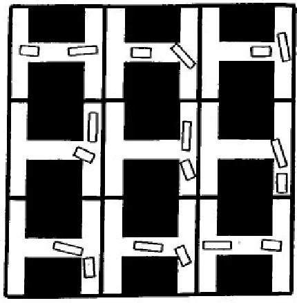
- 6 DOFt-shaped robot in 3D workspace: Figure 3 shows snapshots (from left to right and
top to bottom) along a path generated by RPP for at-shaped robot that can translate and rotate
14 J ´er ˆome Barraquand
Figure 2: Path Generated by RPP for a 3-DOF Rectangular Robot
Figure 3: Path Generated by RPP for a 6-DOFt-Shaped Robot
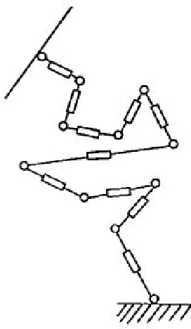
[image:22.612.149.439.351.627.2]Figure 4: Structure of the 10-DOF Non-Serial Manipulator Robot
[image:23.612.161.405.369.622.2]16 J ´er ˆome Barraquand
Figure 6: Structure of the 31-DOF Serial Manipulator Robot
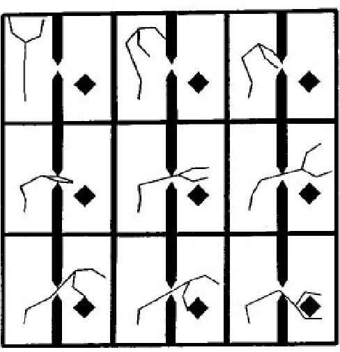
- 10-DOF non-serial manipulator robot in 2D workspace: We also applied RPP to the planar non-serial manipulator robot shown in Figure 4, which includes three prismatic joints (telescopic links) and seven revolute joints. Figure 5 illustrates a path found by RPP. In this example, the potentialU was computed with two control points located at the endpoints of the
two kinematic chains. Overlapping of the links was forbidden. The path was computed in 3 minutes over a 2562bitmap. The size of the corresponding configuration space discretization
is of the order of 1020configurations.
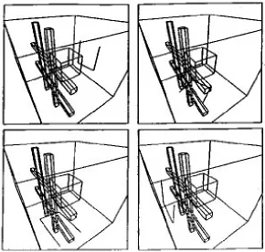
- 31-DOF non-serial manipulator robot in 3D workspace: RPP was also tested on the 31-DOF manipulator illustrated in Figure 6. This manipulator consists of 10 telescopic links connected by 10 spherical joints. The bar at the end of the manipulator is connected to the last link by a revolute joint. A path generated by the program is illustrated in Figure 7. The potential was computed with two control points located at the endpoints of the bar. The computation time was or the order of 15 minutes. The size of the workspace bitmap was 1283. The size of the corresponding configuration space grid is of the order of 1062configurations.
- Coordination of two 3-DOF mobile robots: The same planner was applied to problems requiring the coordination of two 3-DOF mobile robots in a two-dimensional workspace made of several corridors. These are narrow enough so that the two robots cannot pass each other in the same corridor. The two robots are treated by RPP as a single two-body robot with 6 DOF. The problem shown in figure 8 is particularly difficult because the two robots have to interchange their positions in the central corridor; hence, both of them must first move to an intermediate position in order to allow the permutation. Notice that in the initial configuration both robots are rather close from their respective goal configurations, despite the fact that the
Figure 7: Path Generated by RPP for the 31-DOF Serial Manipulator
[image:25.612.177.392.416.635.2]18 J ´er ˆome Barraquand
paths to move there are not short. This example illustrates the power of the random techniques used in RPP. The path was generated in about 30 seconds.
6 Discussion
The experiments with RPP have shown that randomized planning is both efficient and reliable. The efficiency of RPP results from the fact that a typical path planning problem has many solutions, so that a globally random search procedure can find one if it is well-informed most of the time (by the potential function). In fact, similar randomized techniques (e.g. “simulated annealing”) have proven to be useful for solving other NP-hard problems, e.g. the traveling salesman problem (Cerny 1985 [11]) and VLSI placement and routing (Kirkpatrick Gelatt and Vecchi 1983 [23], Sechen 1988 [38]). In these problems the very large search space is associated with a large number of “good” sub-optimal solutions.
Monte-Carlo procedures for optimization have also been used in computer vision. In Geman and Geman 1984 [18], a simulated annealing approach is applied for restoring images blurred with non-linear filters. Several authors have implemented edge detection algorithms based on the same paradigm. Recently, simulated annealing has also been applied to higher-level problems in computer vision. In Barnard 1988 [2], the stereo matching problem is addressed using a hierarchical pixel-level simulated annealing algorithm. A stochastic optimization approach for the three-dimensional reconstruction of stratigraphic layers and the detection of geological faults in seismic data is proposed in Barraquand 1988 [3].
Nevertheless, RPP behaves very differently from the classical simulated annealing procedures. On a sequential computer, while simulated annealing procedures perform a kind of breadth-first search of the graph of local minima of the function to be optimized, RPP performs a depth-first search of this graph using the potential U as the heuristic function. See Barraquand and
Latombe 1989a [6] for a more detailed comparison of RPP and simulated annealing.
Randomized planning has some drawbacks, however. The planner typically generates different paths if it is run several times with the same problem and the running time varies from one run to another. Furthermore, if the input path planning problem admits no solution, the planner has usually no way to recognize it, even after a large amount of computation. Hence, a limit on the running time of the algorithm has to be imposed. But, if this limit is attained and no path has been generated yet, there is no guarantee that no paths exist. However, in practice, experiments have shown that it is not difficult, for a given class of problem (e.g. an object moving in a three-dimensional workspace) and a given size of the configuration space grid, to determine (through a series of preliminary trials) a time limit such that if no path has been found yet, there is little chance that one actually exists.
In Barraquand and Latombe 1989a [6], it has been shown that the randomized planning algorithm implemented in RPP is probabilistically resolution-complete. This result is based on a general property of the Wiener-Levy process: Whenever the free space is connected and bounded, the probability for a Brownian motion! with reflective boundary starting at any
initial configuration q
init
2 Cfree
to reach any given open subset B of Cfree
at least onceduring the interval of time [0;t] converges toward 1 when the durationttends toward infinity.
We can chooseB so that it contain at least one goal configuration and small enough so that it
does not contain a local minimum (other than the goal minimum). From withinB, a gradient
motion achieves a goal configuration. See Barraquand and Latombe 1989a [6] for more detail.
7 Conclusion
This report described a new approach to robot path planning, which essentially consists of: (1) computing potential functions over the robot’s workspace and combining them into a “good” potential function in the configuration space; (2) searching the graph of the local minima of the configuration space potential using an efficient randomization technique; (3) postprocessing the resulting paths in order to generate graceful motions.
This approach has been implemented in a program, called RPP, which was run successfully on many different examples. RPP has solved a large variety of problems that fall far outside the range of the capabilities of any other previous planner, e.g. problems with 10-DOF and 31-DOF robots and multi-robot problems.
20 J ´er ˆome Barraquand
References
1. R.F. Anderson and S. Orey, 1976. Small Random Perturbations of Dynamical Systems with Reflecting Boundary. Nagoya Math. J.. 60:189-216.
2. S.T. Barnard, 1988. Stochastic Stereo Matching Over Scale. Int. J. of Computer Vision. 2(4).
3. J. Barraquand, 1988. Markovian Random Fields in Computer Vision: Applications to
Seismic Data Understanding. Ph.D. Dissertation. Dept. of Computer Vision, INRIA,
Sophia-Antipolis, France (In French.)
4. J. Barraquand, B. Langlois and J.C. Latombe, 1989a. Robot Motion Planning with Many Degrees of Freedom and Dynamic Constraints. In Robotics Research 5. Miura, H. and Arimoto, S. (eds.): MIT Press, pp. 435-444.
5. J. Barraquand, B. Langlois and J.C. Latombe, 1989b. Numerical Potential Field Techniques
for Robot Path Planning, Report No. STAN-CS-89-1285, Dept. of Computer Science,
Stanford University. To appear in IEEE Trans. on Systems, Man, and Cybernetics.
6. J. Barraquand and J.C. Latombe, 1989a. Robot Motion Planning: A Distributed
Represen-tation Approach. Report No. STAN-CS-89-1257. Dept. of Computer Science, Stanford
University. (Also in Int. J. of Robotics Research, 10-6, 1991).
7. J. Barraquand and J.C. Latombe, 1989b. On Nonholonomic Mobile Robots and Optimal Maneuvering. Revue d’Intelligence Artificielle. Hermes. 3(2):77-103. (Also in Proc. of the
4th IEEE Int. Symp. on Intelligent Control, Albany, NY, pp. 340-347.)
8. J. Barraquand and J.C. Latombe, 1991. Non-Holonomic MultiBody Mobile Robots: Controllability and Motion Planning in the Presence of Obstacles. Proc. of the IEEE Int.
Conf. on Robotics and Automation, Sacramento.
9. R.A. Brooks and T. Lozano-P´erez, 1983. A Subdivision Algorithm in Configuration Space for Find-Path with Rotation. Proc. of the 8th Int. Joint Conf. on Artificial Intelligence, Karlsruhe, FRG, pp. 799-806.
10. J.F. Canny, 1988. The Complexity of Robot Motion Planning. MIT Press, Cambridge, MA.
11. V. Cerny, 1985. Thermodynamical Approach to the Traveling Salesman Problem: An Efficient Simulation Algorithm. J. of Optimization Theory and Applications. 45(1):41-51.
12. R. Cliff, 1991. Personal Communication. Lockheed Missiles and Space Company, Inc., Palo Alto, California.
13. B.R. Donald, 1984. Motion Planning with Six Degrees of Freedom. Technical Report 791, Artificial Intelligence Lab., MIT, Cambridge.
14. B. Faverjon, 1984. Obstacle Avoidance Using an Octree in the Configuration Space of a Manipulator. Proc. of the IEEE Int. Conf. on Robotics and Automation, Atlanta, pp. 504-512.
15. B. Faverjon, 1986. Object Level Programming of Industrial Robots. Proc. of the IEEE
Int. Conf. on Robotics and Automation, San Francisco, pp. 1406-1412.
16. B. Faverjon, 1991. Personal Communication. Aleph Technologie, Grenoble, France.
17. B. Faverjon and P. Tournassoud, 1987. A Local Based Approach for Path Planning of Manipulators with a High Number of Degrees of Freedom. Proc. of the IEEE Int. Conf.
on Automation and Robotics, Raleigh, pp. 1152-1159.
18. D. Geman and S. Geman, 1984. Stochastic Relaxation, Gibbs Distributions, and the Bayesian Restoration of Images. IEEE Trans. on Pattern Analysis and Machine
Intelli-gence. PAMI-6:721-741.
19. S. Geman and C.R. Hwang, 1986. Diffusions for Global Optimization. SIAM J. on Control
and Optimization. 24(5).
20. L. Gouz`enes, 1984. Strategies for Solving Collision-Free Trajectories Problems for Mobile and Manipulator Robots. Int. J. of Robotics Research, 3(4):51-65.
21. Graux, Kociemba, Millies. 1991. M´ethode de planification de trajectoires appliqu´ee `a la
robotique. A´erospatiale, Centre de recherches de Suresnes, France (in French).
22. O. Khatib, 1986. Real-Time Obstacle Avoidance for Manipulators and Mobile Robots.
Int. J. of Robotics Research. 5(1):90-98.
23. S. Kirkpatrick, C.D. Gelatt and M.P. Vecchi, 1983. Optimization by Simulated Annealing.
Science. 220:671-680.
24. P. Khosla and R. Volpe, 1988. Superquadric Artificial Potentials for Obstacle Avoidance and Approach. Proc. of the IEEE Int. Conf. on Robotics and Automation, Philadelphia, PA, 1178-1784.
25. D.E. Koditschek, 1987. Exact Robot Navigation by Means of Potential Functions: Some Topological Considerations. Proc. of the IEEE Int. Conf. on Robotics and Automation, Raleigh, pp. 1-6.
26. J.C. Latombe, 1990. Robot Motion Planning. Kluwer Academic Publishers, Boston.
27. C. Laugier and F. Germain, 1985. An Adaptive Collision-Free Trajectory Planner. Int.
Conf. on Advanced Robotics, Tokyo, Japan.
28. V. Libby, 1990a. Use of Window Addressable Memories for High Speed Geometrical Analysis. IEEE Journal of VLSI Signal Processing.
29. V. Libby, 1990b. Sensor Data Integration for Real-Time Environment Analysis. Proc. of
22 J ´er ˆome Barraquand
30. T. Lozano-P´erez, 1983. Spatial Planning: A Configuration Space Approach. IEEE Trans.
on Computers. C-32(2):108-120.
31. T. Lozano-P´erez, 1987. A Simple Motion-Planning Algorithm for General Robot Manip-ulators. IEEE J. of Robotics and Automation. RA-3(3):224-238.
32. C. M´etivier and R. Urbschat, 1990. Run-Time Statistical Analysis of a Robot Motion
Planning Algorithm. Internal Technical Note, Robotics Lab., Computer Science Dept.,
Stanford University.
33. C. ´O’D´unlaing, M. Sharir and C.K. Yap, 1983. Retraction: A New Approach to Motion Planning. Proc. of the 15th ACM Symp. on the Theory of Computing, Boston, pp. 207-220.
34. K. Ohlund, 1990. Personal Communication. Lockheed Missiles and Space Company, Inc., Palo Alto, California.
35. A. Papoulis, 1965. Probability, Random Variables, and Stochastic Processes. Mc. Graw-Hill.
36. E. Rimon and D.E. Koditschek, 1989. The Construction of Analytic Diffeomorphisms for Exact Robot Navigation on Star Worlds. Proc. of the IEEE Int. Conf. on Robotics and
Automation, Scottsdale, pp. 21-26.
37. J.T. Schwartz and M. Sharir, 1983. On the ‘Piano Movers’ Problem: II. General Techniques for Computing Topological Properties of Real Algebraic Manifolds. Advances in Applied
Mathematics. Academic Press 4, pp. 298-351.
38. C. Sechen, 1988. VLSI Placement and Routing Using Simulated Annealing, Kluwer Academic Publishers.
39. D. Zhu and J.C. Latombe, 1989. New Heuristic Algorithms for Efficient Hierarchical
Path Planning, Report No. STAN-CS-89-1279, Dept. of Computer Science, Stanford
University. (To appear in IEEE Trans. on Robotics and Automation.)
The following documents may be ordered by regular mail from:
Librarian – Research Reports Digital Equipment Corporation Paris Research Laboratory 85, avenue Victor Hugo 92563 Rueil-Malmaison Cedex France.
It is also possible to obtain them by electronic mail. For more information, send a message whose subject line [email protected], from within Digital, todecprl::doc-server.
Research Report 1: Incremental Computation of Planar Maps. Michel Gangnet, Jean-Claude Herv ´e, Thierry Pudet, and Jean-Manuel Van Thong. May 1989.
Research Report 2: BigNum: A Portable and Efficient Package for Arbitrary-Precision Arithmetic. Bernard Serpette, Jean Vuillemin, and Jean-Claude Herv´e. May 1989.
Research Report 3: Introduction to Programmable Active Memories. Patrice Bertin, Didier Roncin, and Jean Vuillemin. June 1989.
Research Report 4: Compiling Pattern Matching by Term Decomposition. Laurence Puel and Asc ´ander Su ´arez. January 1990.
Research Report 5: The WAM: A (Real) Tutorial. Hassan A¨ıt-Kaci. January 1990.
Research Report 6: Binary Periodic Synchronizing Sequences. Marcin Skubiszewski. May 1991.
Research Report 7: The Siphon: Managing Distant Replicated Repositories. Francis J. Prusker and Edward P. Wobber. May 1991.
Research Report 8: Constructive Logics. Part I: A Tutorial on Proof Systems and Typed
-Calculi. Jean Gallier. May 1991.
Research Report 9: Constructive Logics. Part II: Linear Logic and Proof Nets. Jean Gallier. May 1991.
Research Report 12: Residuation and Guarded Rules for Constraint Logic Programming. Gert Smolka. June 1991.
Research Report 13: Functions as Passive Constraints in LIFE. Hassan A¨ıt-Kaci and Andreas Podelski. June 1991 (Revised, November 1992).
Research Report 14: Automatic Motion Planning for Complex Articulated Bodies. J ´er ˆome Barraquand. June 1991.
Research Report 15: A Hardware Implementation of Pure Esterel. G ´erard Berry. July 1991.
Research Report 16: Contribution `a la R ´esolution Num ´erique des ´Equations de Laplace et de la Chaleur. Jean Vuillemin. February 1992.
Research Report 17: Inferring Graphical Constraints with Rockit. Solange Karsenty, James A. Landay, and Chris Weikart. March 1992.
Research Report 18: Abstract Interpretation by Dynamic Partitioning. Fran¸cois Bourdoncle. March 1992.
Research Report 19: Measuring System Performance with Reprogrammable Hardware. Mark Shand. August 1992.
14
A
u
to
ma
tic
M
ot
io
n
P
la
nni
ng
fo
r
C
ompl
e
x
A
rt
ic
u
la
te
d
B
odi
e
s
J ´er ˆom e B arraquandd i g i t a l
PARIS RESEARCH LABORATORY
85, Avenue Victor Hugo