CRL 97 3 pdf

(1)

TM

Semiautomatic Methods for Recovering Radial Distortion Parameters from A Single Image

Sing Bing Kang

CRL 97/3

(2)

Cambridge Research Laboratory

The Cambridge Research Laboratory was founded in 1987 to advance the state of the art in both core computing and human-computer interaction, and to use the knowledge so gained to support the Company’s corporate objectives. We believe this is best accomplished through interconnected pur-suits in technology creation, advanced systems engineering, and business development. We are ac-tively investigating scalable computing; mobile computing; vision-based human and scene sensing; speech interaction; computer-animated synthetic persona; intelligent information appliances; and the capture, coding, storage, indexing, retrieval, decoding, and rendering of multimedia data. We recognize and embrace a technology creation model which is characterized by three major phases:

Freedom: The life blood of the Laboratory comes from the observations and imaginations of our

research staff. It is here that challenging research problems are uncovered (through discussions with customers, through interactions with others in the Corporation, through other professional interac-tions, through reading, and the like) or that new ideas are born. For any such problem or idea, this phase culminates in the nucleation of a project team around a well articulated central research question and the outlining of a research plan.

Focus: Once a team is formed, we aggressively pursue the creation of new technology based on

the plan. This may involve direct collaboration with other technical professionals inside and outside the Corporation. This phase culminates in the demonstrable creation of new technology which may take any of a number of forms - a journal article, a technical talk, a working prototype, a patent application, or some combination of these. The research team is typically augmented with other resident professionals—engineering and business development—who work as integral members of the core team to prepare preliminary plans for how best to leverage this new knowledge, either through internal transfer of technology or through other means.

Follow-through: We actively pursue taking the best technologies to the marketplace. For those

opportunities which are not immediately transferred internally and where the team has identified a significant opportunity, the business development and engineering staff will lead early-stage com-mercial development, often in conjunction with members of the research staff. While the value to the Corporation of taking these new ideas to the market is clear, it also has a significant positive im-pact on our future research work by providing the means to understand intimately the problems and opportunities in the market and to more fully exercise our ideas and concepts in real-world settings.

Throughout this process, communicating our understanding is a critical part of what we do, and participating in the larger technical community—through the publication of refereed journal articles and the presentation of our ideas at conferences–is essential. Our technical report series supports and facilitates broad and early dissemination of our work. We welcome your feedback on its effec-tiveness.

(3)

Semiautomatic Methods for Recovering Radial Distortion

Parameters from A Single Image

Sing Bing Kang

May 1997

Abstract

In this technical report, we address the problem of recovering the camera radial distortion coefficients from one image. In particular, we present three interactive methods where the user indicate lines in the single image. The first method is the most direct: the manually chosen points are used to compute the radial distortion parameters. The second and third methods allow the user to draw snakes on the image, with each approximately corresponding to a projected straight line in space. These snakes are drawn to strong edges subject to regularization. The difference between these two methods is the behavior of the snakes. In one of the last two methods, they behave like independent, conventional snakes. In the other method, their behavior are globally connected via a consistent model of image radial distortion. We call such snakes radial distortion snakes.

(4)

c Digital Equipment Corporation, 1997

This work may not be copied or reproduced in whole or in part for any commercial purpose. Per-mission to copy in whole or in part without payment of fee is granted for nonprofit educational and research purposes provided that all such whole or partial copies include the following: a notice that such copying is by permission of the Cambridge Research Laboratory of Digital Equipment Corpo-ration in Cambridge, Massachusetts; an acknowledgment of the authors and individual contributors to the work; and all applicable portions of the copyright notice. Copying, reproducing, or repub-lishing for any other purpose shall require a license with payment of fee to the Cambridge Research Laboratory. All rights reserved.

CRL Technical reports are available on the CRL’s web page at http://www.crl.research.digital.com.

Digital Equipment Corporation Cambridge Research Laboratory One Kendall Square, Building 700

(5)

CONTENTS i

List of Figures

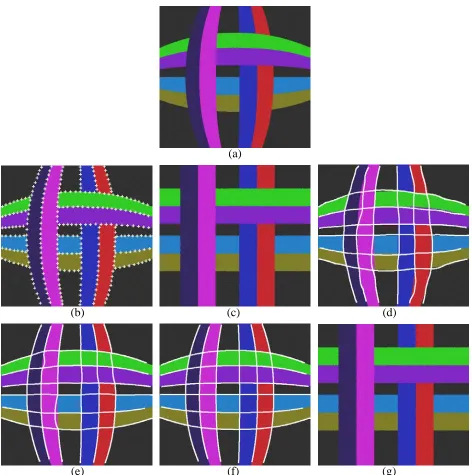
1 Synthetic image with no image noise: (a) Original image, (b) Manually selected points (299 points), (c) Undistorted image from (b), (d) Manually drawn lines, (e) After applying conventional snake algorithm, (f) After applying radial distortion snake algorithm, (g) Undistorted image from (f) (very similar to results from (e)). . 11

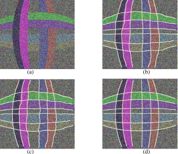
2 Synthetic image with image gaussian noise with standard deviation of 100 intensity levels: (a) Original image, (b) Manually drawn lines, (c) After applying conven-tional snake algorithm, (d) After applying radial distortion snake algorithm. . . 12

3 Graphs showing the effect of gaussian image noise (standard deviation in intensity level) on recovered radial distortion parameters: (a) ₁(true value is10

;6

), and (b)

2 (true value is10 ;10

). Note that for the manual method, the points were placed on the image with no noise. Also, for the other two methods, the snakes were initialized on the image with no noise. . . 13

4 Graph showing the effect of gaussian image noise (standard deviation in intensity level) on RMS undistortion error

E

RMS. . . 14 5 Office scene (manual): (a) Original distorted image, (b) Selected points, (c)

Undis-torted image. . . 15

6 Office scene (using conventional snakes): (a) Chosen snakes, (b) Final snake con-figuration, (c) Undistorted image. Note the relatively uneven snake to the left of image in (b). . . 15

7 Office scene (using radial distortion snakes): (a) Chosen snakes, (b) Final snake configuration, (c) Undistorted image. Notice the smoother snakes compared to Figure 6. . . 15

8 Office scene (comparing the two snake implementation): (a) Initial snake con-figuration, and final snake configuration for (b) Conventional snakes, (c) Radial distortion snakes. . . 16

9 Another example: (a) Original image, (b) Initial snake configuration, and final snake configuration for (c) Conventional snakes, (e) Radial distortion snakes. The respective undistorted images are (d) and (f). Note that the snakes are shown in black here. . . 17

(7)

LIST OF TABLES iii

List of Tables

(8)

(9)

1

1 Introduction

Most cameras having wide fields of view suffer from non-linear distortion due to simplified lens construction and lens imperfection. Applications that require 3-D modeling of large scenes (e.g., [1, 10, 18]) or image compositing over a large scene area (e.g., [13, 16, 17]) typically use cameras with such wide fields of view. In such instances, the camera distortion effect has to be removed by calibrating the camera and subsequently undistorting the input image.

In general, there are two forms of camera distortion, namely radial distortion and tangential distortion. In this technical report, we address the problem of recovering the camera radial distortion coefficients from one image. In particular, we present three interactive methods where the user indicate lines in the single image. The first method is the most direct: the manually chosen points are used to compute the radial distortion parameters. The second and third methods allow the user to draw snakes on the image, with each approximately corresponding to a projected straight line in space. These snakes are drawn to strong edges subject to regularization. The difference between these two methods is their behavior. In one of the last two methods, they behave like independent, conventional snakes. In the other method, their behavior are globally connected via a common model of image radial distortion. Such snakes are termed radial distortion snakes. These methods, and in particular the one that uses radial distortion snakes, are especially useful in cases where only one image is available and straight 3-D lines are known to exist in the scene.

In many cases, camera parameter recovery is disconnected from the feature detection process. While this does not present a problem if the feature detection is correct, directly linking the feature detection to parameter estimation results in more robust recovery, especially in the presence of noise. The spirit of this work is very much linked to this philosophy.

1.1 Prior work

There has been significant work done on camera calibration, but many of them require a specific calibration pattern with known exact dimensions. There is a class of work done on calibrating the camera using the scene image or images themselves, and possibly taking advantage of special structures such as straight lines, parallel straight lines, perpendicular lines, and so on. One relevant work that belong to this class is that of Becker and Bove [1]. They use the minimum vanishing point dispersion constraint to estimate both radial and decentering (or tangential) lens distortion. The user has to group parallel lines together.

(10)

2 2 FINDING THE RADIAL DISTORTION PARAMETERS

fit function. The points on the plumb lines were extracted manually; the measuring process was quoted as consuming between 5-6 hours for 162 points from horizontal lines and 162 from vertical lines!

Stein [15] uses point correspondences between multiple views to extract radial distortion coef-ficients. He uses epipolar and trilinear constraints and searches for the amount of radial distortion that minimizes the errors in these constraints.

Photogrammetry methods usually rely on using known calibration points or structures [2, 3, 6, 20]. Tsai [20] uses corners of regularly spaced boxes of known dimensions for full camera calibration. In a more flexible arrangement, Faig [6] requires that the points used only be coplanar, and that there are identified horizontal and vertical points among these points. Wei and Ma [21], on the other hand, use projective invariants to recover radial distortion coefficients.

The idea of active deformable contours, or snakes, was first described in [11]. Since then, there has been numerous papers on the applications and refinement of snakes. Snakes has been applied to, for example, from tracking human facial features [22] and cells [4] to reconstruction of objects [19]. The various forms of snakes include the notion of “inflating contour” to reduce sensitivity to initialization (but at the expense of increase in parameters) [5], and the “dual active contour” [8]. In all these cases, the snakes, some of which may be parameterized, work independently of each other. In one of our proposed methods, the snakes are globally parameterized, and they deform in a globally consistent manner.

1.2 Organization

In Section 2, we briefly describe the radial distortion equation before presenting the three interac-tive methods of recovering the distortion parameters from one image. Subsequently, we present results using synthetic and real images in Section 3. In the same section, we propose a metric for comparing accuracy of recovered radial distortion parameters. The methods are compared and discussed in Section 4, with a summary and directions for future research given in Section 5.

2 Finding the radial distortion parameters

(11)

2.1 The radial distortion equation 3

2.1 The radial distortion equation

The modeling of lens distortion can be found in [14]. In essence, there are two kinds of lens distortion, namely radial and tangential (or decentering) distortion. Each kind of distortion is represented by an infinite series, but generally, a small number is adequate.

According to Brown [2], the lens distortion equations are

x

u =

x

d+

x

d 1 X

l=1 l

R

ld+

u

y

u)

is the theoretical undistorted image point location,(

x

d

y

d 1 X

l=1 l

R

ld

y

u =

y

d+

y

d 1 X

l=1 l

R

ld (2)

In our proposed calibration methods (each of which using only a single image), we expect the user to indicate the image locations of the projected straight lines in the scene. The most direct way possible is to directly on the edges and have the radial distortion parameters computed automatically.

2.2 Method 1: Using user-specified points

This method comprises two stages:

Manual stage—the user select points on lines by clicking directly on the image,

Automatic stage–the camera radial distortion parameters are computed using a least-squares

(12)

The radial distortion parameters are recovered by minimizing the objective function

E =

Nline

X i=1

Nptsi

X j=1

"

(cos

i

x

ij+sin

i

y

ij)(1+ L X

l=1 l

R

lij

);

i #2

E1 =

Nline

X i=1

Nptsi

X j=1

"

y

ij;

m

i

x

ij;

c

i 1+

P

Ll=1 l

R

lij

#2

(4)

for lines whose inclinations are closer to the horizontal axis, or

E2 =

Nline

X i=1

Nptsi

X j=1

"

x

ij;

m

0

i

y

ij;

c

0 i 1+

P

Ll=1 l

R

lij

#2

(5)

for lines whose inclinations are closer to the vertical axis. The choice betweenE1 andE2 is made

based on the slope of the best fit line through the set of distorted points. Taking the partials of (4) with respect to

c

nand

m

nand solving yields

S

n(1) PN

ptsn

j=1

x

2nj;

S

2n(

x

)

(6)

where

S

n(

f

)=

Nptsn

X j=1

f

j 1+

P

Ll=1 l

R

lnj (7)

0

n(1) PN

ptsn

j=1

n(1)

(9)

The (

m

n

c

n) and (

m

0

n

c

0

n) representations are then converted to (

n

n) line representation as

(13)

2.2 Method 1: Using user-specified points 5

later (compare (3), where(

i

i)’s are known, with (18)). l’s can be found by solving the set of

simultaneous linear equations

L X

l=1 l

G

m+l =

H

m;

G

m (10)

with

m

=1

:::L

, and

G

m =

Nline

X i=1

Nptsi

X

j=1

g

2ij

R

mij

H

m =

Nline

X

i=1

i

Nptsi

X

j=1

g

ij

R

mij (11)

g

ij = cos

i

x

ij+sin

i

y

ij

For the special case of estimating only one radial distortion coefficient (i.e.,

L

=1),

1 =

H

1;

G

1

G

2 (12)

For the case of two radial distortion coefficients (i.e.,

L

=2),

0 @ 1 2 1 A = 0

A (13)

An alternative would be to employ the iterative gradient-descent technique involving the first order Taylor’s expansion of the line fit function [3].

The problem with this approach is that it can be rather manually intensive. Typically, the extracted radial distortion parameters are more reliable with more (carefully) chosen points.

The other two methods described in the subsequent two subsection, the user draws curves over projected straight lines. The drawn curves need not be very accurate. Once this is done, these algorithms automatically reshape the snakes to stick to edges and compute the radial distortion parameters based on the final snake configuration. The difference between the these two methods is in the formulation of the snakes.

(14)

2.3 Method 2: Using conventional snakes

In this method, the motion of the snakes is based on two factors: motion smoothness (due to external forces) and spatial smoothness (due to internal forces). Given the original configuration of a snake, a point on the snakepj moves by the amount

pj at each step given by

pj =(1;

) X

k2Nj

jk

pedgek+

X

k2N

0 j

0

jk(pk;pj) (14)

where Nj and N 0

j are the neighborhood of pixel at pj, including pj.

pedgei is the computed

motion of the

i

th point towards the nearest detectable edge, with its magnitude being inversely proportional to its local intensity gradient (only when it is not close to zero).

jk and

0

jk are the respective neighborhood weights.

is set according to the emphasis on motion coherency and spatial smoothness. In our implementation,Nj =N

0

j, the radius of the neighborhood being 5 and the weights

_jk =

0

jkbeingf1

2

4

8

16

32

16

8

4

2

1g.

Once the snakes have settled, the camera radial distortion parameters are recovered using the least-squares formulation. Note that a very simplistic version of the snake is implemented here. The intent is to compare the effect of having snakes that operate independently of each other behaves worse in general than those which act in a global manner (as in Method 3 below), given the constraints of the types of curves that they are collectively attempt to seek.

2.4 Method 3: Using radial distortion snakes

Using conventional snakes have the problem of getting stuck on wrong local minima. This problem can be reduced by imposing more structure on the snake—namely, the shape of the snake has to be consistent with the expected distortion of straight lines due to global radial distortion. For this reason, we call such snakes radial distortion snakes.

The complexity of the original objective function can be reduced if we consider the fact that the

effect of radial distortion is rotationally invariant about the principal point, ignoring asymmetric

distortions due to tangential distortion and non-unit aspect ratio. This method has the following steps:

1. For each snake, find the best fit line,

(15)

2.4 Method 3: Using radial distortion snakes 7

3. Estimate best fit set of radial distortion parameters ₁

:::

L from the rotated set of lines (described shortly).

4. Find the expected rotated distorted pointp 0

j =(

x

j

y

j), whose undistorted version lies on a

horizontal line, i.e.,

y

j " 1+ L X l=1 l

(

x

2j+

y

2j )l

#

=

h

(15)

Given the initial points(

x

(0)

j

y

j(0)), we take

x

j =

x

(0)

j and iteratively compute

y

5. Update points using current best estimate of ’s and edge normal. In other words, the point

pj is updated based on

pnew_j = p

kappa

j +(1;

)pnormal_j ₍₁₇₎

with0 1.

pnormal_j _{is the expected new position of the snake point using Method 2}

described earlier (see (14)). For the

i

th snake,p kappa

j is obtained by rotatingp 0

j (calculated from the previous step) about the principal point by(;

i).

6. Iterate all the above steps until overall mean change is negligible, or for a fixed number of iterations. The latter condition is adopted in our work.

In (17), = 0is equivalent to moving the points according to the usual snake behavior as

in Method 2 (function of edge normal, edge strength, smoothness, and continuity), while = 1

is equivalent to moving to a position consistent to the current estimated radial distortion. From experiments, setting = 1has the effect of slower convergence, and in some cases, convergence

to a wrong configuration. In general, may be time-varying, for example, with = 0initially

and gradually increasing to 1. n our case, we set the time-varying function of to be linear from 0 to 1 with respect to the preset maximum number of iterations.

To find the radial distortion parameters _l’s given rotated coordinates, we minimize the objec-tive function

E =

Ns

X i=1

Nptsi

X

j=1

!

ij

"

y

ij 1+ L X

l=1 l

R

lij

! ;

h

i

#2

(18)

where

N

_sis the number of snakes,

R

_ij =

x

2ij+

y

2ijand

!

ijis the confidence weight associated with

(16)

(

x

ij

y

ij). We use the rotated versions in order to simplify the analysis of the objective function to

a point where a direct closed form solution is possible.

Taking the partial derivatives with respect to the unknown parameters and equating them to zero, we get

@

E

@h

m =0)

h

m =

1 PN

ptsm

j=1

!

E

@

n =2

Ns

X i=1

Nptsi

X

j=1

!

ij

"

y

ij 1+ L X

l=1 l

R

lij

! ;

h

i

#

y

ij

R

nij =0 (20)

for

n

=1

:::L

, which yields

Ns

X i=1

Nptsi

X

j=1

!

ij

y

2ij

R

nij

1+

L X

l=1 l

R

lij

! =

Ns

X

i=1

h

i

Nptsi

X

j=1

!

y

2ij

R

nij (22)

and rearranging the summation in the LHS of (21), we get

LHS =

A

n+ L X l=1 l Ns X i=1

Nptsi

X

j=1

!

ij

y

2ij

R

l+n ij

=

A

n+ L X

l=1 l

A

l+n (23)

As for the RHS of (21), substituting for

h

ifrom (19) and changing the summation subscript in the last summation term to avoid confusion, we get

RHS = Ns X i=1 1 PN ptsi

j=1

!

ij

Nptsi

X

j=1

!

ij

y

ij

1+

L X

l=1 l

R

lij

!N ptsi X

J=1

!

iJ

y

iJ

R

niJ

= Ns X i=1 0 @

y

i+ 1 PN

ptsi

Nptsi

X

J=1

!

iJ

y

iJ

R

niJ

(17)

9 = Ns X i=1

y

i

Nptsi

X

J=1

!

iJ

y

iJ

R

niJ

+ L X l=1 l Ns X i=1 1 PN ptsi

j=1

!

ij

Nptsi

X

j=1

!

ij

y

ij

R

lij

Nptsi

X

J=1

!

iJ

y

iJ

R

niJ

=

C

n+ L X

l=1 l

D

ln (24)

for

n

=1

:::L

.

From (23) and (24), after rearranging, we get

L X

l=1 l

(

A

l+n;

D

ln)=

C

n;

A

n (25)

;1 0 @

(

C

1;

A

1) (

C

2;

A

2)

1

A (27)

For

L >

1, we estimate the ’s in succession. In other words, we first estimate 1, followed by 1and 2, and so on, up til the last stage where we estimate all the radial distortion parameters 1, ..., L.

3 Results

In this section, we present results from both synthetic and real images. The synthetic images are used to verify the accuracy of the recovered radial distortion parameters. We also artificially incorporate image noise to study the effects of noise on the snakes. Real images with significant radial distortion are used to illustrate their use in practice. For all the experiments described in this section, we recover ₁ and ₂ only, i.e., we set

L

= 2. This is generally sufficient for low to

moderately distorted images in practice.

3.1 Metric for accuracy

(18)

10 3 RESULTS

different sets of l’s may give rise to visually similar undistorted images. In addition, coming up with an error metric using only the actual and estimated sets of l’s is not trivial. In such a situation, it is more reasonable to compute an image distance-based metric that is a function of the error in undistorting the image using the actual and estimated sets of radial distortion parameters. A reasonable error measure is the RMS difference

E

RMS between the predicted and the estimated undistorted coordinates (based on actual and estimated radial distortion parameters respectively). The error measure

E

RMS is given by

E

RMS = v u u u u t 1

HW

H 2 X

r=;H

2 W

2 X

c=;W

2

x

act_{u rc};

x

estu rc 2

+

y

act_{u rc};

y

u rcest

2 = v u u u u t 1

HW

H 2 X

r=;H

2 W

2 X

c=;W

2

c

2+

r

2] "

L X l=1

( actl ; estl )(

c

2+

r

2)l #2 (28) = v u u u u t 1

HW

H 2 X

r=;H

2 W

2 X

c=;W

2

R

d rc "

L X

l=1

l

R

ld rc

#2

where

H

and

W

are the image height and width respectively,

R

d rc =

c

2

+

r

2_{, and}

_l

= actl ; est

l . We use the superscripts

act

and

est

to denote actual and estimated values respectively, and subscripts

u

and

d

to denote undistorted and distorted values respectively.

3.2 Experiments using synthetic images

In our first set of experiments, we use synthetic images containing straight lines and distort them with known radial distortion parameters. In addition, we vary the image noise to see how it af-fects both the conventional and radial distortion snake algorithms. In particular, the actual radial distortion parameters corresponding to ₁ = 10

;6

and ₂ = 10 ;10

are applied to images with a resolution of480512. The gaussian image noise (specified by the standard deviation in intensity

level) is varied from 0 to 100 intensity levels. Figure 1 shows the results for the case with no image noise using all three methods, and Figure 2 shows results for the same test image with image noise of 100. It is clear from Figure 2 that the radial distortion snakes yielded a better result than that of conventional snakes.

(19)

3.2 Experiments using synthetic images 11

(a)

(b) (c) (d)

[image:19.612.71.543.117.592.2]

(e) (f) (g)

(20)

12 3 RESULTS

(a) (b)

[image:20.612.126.485.208.520.2]

(c) (d)

(21)

3.3 Experiments using real images 13

0.0 20.0 40.0 60.0 80.0 100.0

Image noise −0.5 0.0 0.5 1.0 1.5 2.0 2.5 kappa1 (x1.0e−6) True Conventional snakes Radial distortion snakes Manually placed points Manually placed lines

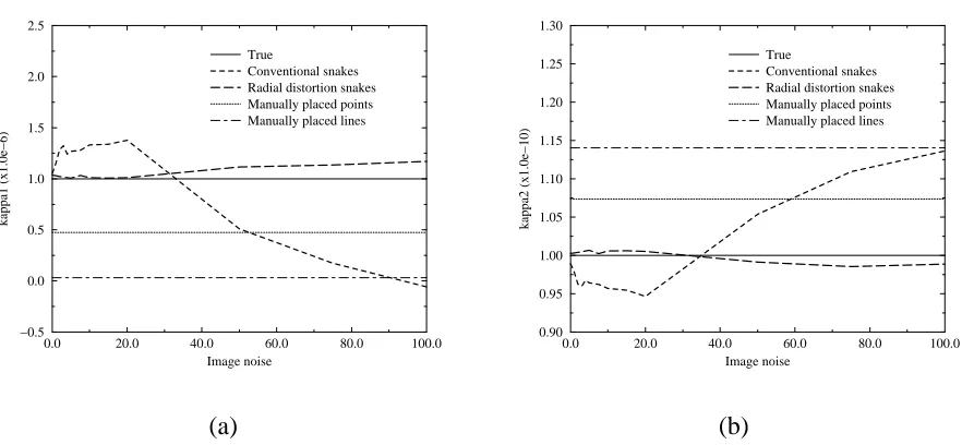
0.0 20.0 40.0 60.0 80.0 100.0

Image noise 0.90 0.95 1.00 1.05 1.10 1.15 1.20 1.25 1.30 kappa2 (x1.0e−10) True Conventional snakes Radial distortion snakes Manually placed points Manually placed lines

[image:21.612.85.526.114.318.2]

(a) (b)

Figure 3: Graphs showing the effect of gaussian image noise (standard deviation in intensity level) on recovered radial distortion parameters: (a) ₁ (true value is 10

;6

), and (b) ₂ (true value is

10 ;10

). Note that for the manual method, the points were placed on the image with no noise. Also, for the other two methods, the snakes were initialized on the image with no noise.

noise levels, both snake algorithms exhibit reasonable robustness to image noise. However, the radial distortion snake algorithm is even more stable despite the presence of high image noise, in comparison to the conventional snake algorithm. Note that both snake algorithms have essentially the same implementation and uses the same edge gradient estimation and same maximum number of 200 steps or iterations. The difference with the radial distortion snake is that all of the radial dis-tortion snakes are globally connected via a common set of estimated radial disdis-tortion parameters. As a frame of reference, the radial distortion parameters that are estimated based directly from the user drawn lines ( 1 =3

:

2210

;8

and 2 =1

:

1410 ;10

) yield an RMS pixel location error of 4.15.

3.3 Experiments using real images

(22)

14 3 RESULTS

0.0 20.0 40.0 60.0 80.0 100.0

Image noise 0.0

1.0 2.0 3.0 4.0 5.0 6.0

RMS pixel error

[image:22.612.185.430.125.327.2]

Conventional snakes Radial distortion snakes Manually placed points Manually placed lines

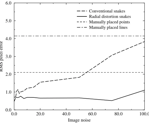
Figure 4: Graph showing the effect of gaussian image noise (standard deviation in intensity level) on RMS undistortion error

E

_RMS.

illustrates a situation where the radial distortion snakes appear to have converged to a more optimal local minima than that of conventional snakes for the same snake initialization. This example shows that the radial distortion snakes are more tolerant to errors in snake initialization by the user.

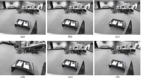
Another example involving a real image is shown in Figure 9. This scene is a more difficult one due to the relative sparseness of structurally straight and long lines within the camera viewing space. As a result, the recovery of the radial distortion parameters are more sensitive to errors in the extracted curves. This is evidenced by Figure 9(d) for the conventional snake algorithm, where slight errors have resulted in significantly erroneous estimates in the radial distortion parameters.

Method ₁ ₂

Manual 2

:

9310

3.3 Experiments using real images 15

[image:23.612.78.541.114.246.2]

(a) (b) (c)

Figure 5: Office scene (manual): (a) Original distorted image, (b) Selected points, (c) Undistorted image.

[image:23.612.80.540.308.441.2]

(a) (b) (c)

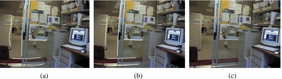
Figure 6: Office scene (using conventional snakes): (a) Chosen snakes, (b) Final snake configura-tion, (c) Undistorted image. Note the relatively uneven snake to the left of image in (b).

(a) (b) (c)

[image:23.612.75.543.504.636.2]

(24)

16 4 DISCUSSION

[image:24.612.75.539.109.243.2]

(a) (b) (c)

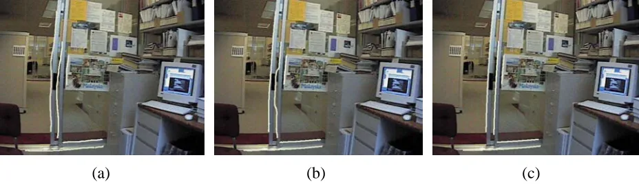
Figure 8: Office scene (comparing the two snake implementation): (a) Initial snake configuration, and final snake configuration for (b) Conventional snakes, (c) Radial distortion snakes.

On the other hand, the radial distortion snake algorithm resulted in a visually more correct undis-torted image.

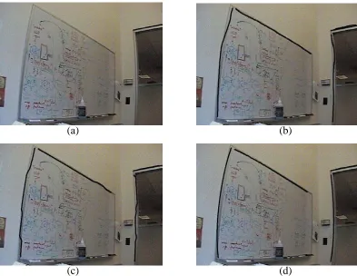
Radial distortion snakes appear to have the effect of widening the range of convergence com-pared to conventional snakes (as exemplified by Figure 8). It is reasonable to hypothesize that radial distortion snakes have fewer false local minima, although this number will increase with the number of radial distortion parameters to be estimated. An example of radial distortion snakes converging to a wrong local minima is shown in Figure 10. As can be seen, due to the rather bad placing of the initial snakes (specifically the two most vertical ones), the snakes in both implemen-tations converged to straddle different parallel edges, causing incorrect estimated radial distortion parameters.

4 Discussion

The first method of manually picking discrete direct line points is the simpliest to implement and understand, but of all the three methods described, it is the most burdensome to the user. In our implementation, the user has to be relatively careful in choosing the points. This is because the user-designated input locations are used directly in the radial distortion parameter estimation step. One can, however, add the intermediate process of automatic local edge searching and location refinement, but this may pose a problem in an image of a complicated scene with many local edges.

(25)

17

(a) (b) (c)

[image:25.612.74.538.108.364.2]

(d) (e) (f)

Figure 9: Another example: (a) Original image, (b) Initial snake configuration, and final snake configuration for (c) Conventional snakes, (e) Radial distortion snakes. The respective undistorted images are (d) and (f). Note that the snakes are shown in black here.

distortion snakes find best adaptation according to best global fit to radial distortion parameters. They appear to have fewer false local minima in comparison to conventional snakes, and are less prone to being trapped in bad local minima. At every step, the radial distortion snakes act together to give an optimal estimate of the global radial distortion parameters and deform in a consistent manner in approaching edges in the image.

(26)

18 4 DISCUSSION

(a) (b)

[image:26.612.107.500.211.515.2]

(c) (d)

(27)

19

5 Summary and future work

We have described three semiauthomatic methods for estimating radial distortion parameters from a single image. All the methods rely on the user indicating the edges of projected straight lines in space on the image. The first requires good user point to point localization while the other two only requires approximate initial snake configurations.

In essence, all the methods use the point locations to estimate the radial distortion parameters based on least-squares minimization technique. However, the last two methods automatically de-forms the snakes to adapt and align along to strong edges subject to regularization. In the second method, the snakes behave independently and in a conventional way with internal smoothing con-straints and external edge-seeking forces. In the third method, the snakes (called radial distortion snakes) behave coherently to external edge-seeking forces and more importantly, directly linked to the image radial distortion model. As a result, this method is more robust and accurate than the other two methods.

One direction for future work is to extend this work to estimate the principal point and tan-gential (or decentering) distortion parameters in addition to the radial distortion parameters. This would come at the expense of higher complexity and potential instability or problems in conver-gence. Another area is to fully automate the process of determining radial distortion by edge detection and linking, followed by hypothesis and testing. A robust estimator may be used to reject outliers (e.g., RANSAC-like algorithm [7]).

References

[1] S. Becker and V. B. Bove. Semiautomatic 3-D model extraction from uncalibrated 2-D cam-era views. In Proc. SPIE Visual Data Exploration and Analysis II, volume 2410, pages 447–461, February 1995.

[2] D. C. Brown. Decentering distortion of lenses. Photogrammetric Engineering, 32(3):444– 462, May 1966.

[3] D. C. Brown. Close-range camera calibration. Photogrammetric Engineering, 37(8):855– 866, August 1971.

(28)

20 REFERENCES

[5] L. D. Cohen and I. Cohen. Finite-element methods for active contour models and balloons for 2-D and 3-D images. IEEE Transactions on Pattern Analysis and Machine Intelligence, 15(11):1131–1147, November 1993.

[6] W. Faig. Calibration of close-range photogrammetry systems: Mathematical formulation.

Photogrammetric Engineering and Remote Sensing, 41(12):1479–1486, December 1975.

[7] M.A. Fischler and R.C. Bolles. Random sample consensus: A paradigm for model fitting with applications to image analysis and automated cartography. Communications of the ACM, 24(6):381–395, June 1981.

[8] S. R. Gunn and M. S. Nixon. A robust snake implementation; A dual active contour. IEEE

Transactions on Pattern Analysis and Machine Intelligence, 19(1):63–68, January 1997.

[9] K. Ikeuchi and M. Hebert. Task oriented vision. In Image Understanding Workshop, pages 497–507, Pittsburgh, Pennsylvania, September 1990. Morgan Kaufmann Publishers.

[10] S. B. Kang and R. Szeliski. 3-D scene data recovery using omnidirectional multibaseline stereo. In Proc.s IEEE Computer Society Conference on Computer Vision and Pattern

Recog-nition, pages 364–370, June 1996.

[11] M. Kass, A. Witkin, and D. Terzopoulos. Snakes: Active contour models. In First

Interna-tional Conference on Computer Vision (ICCV’87), pages 259–268, London, England, June

1987. IEEE Computer Society Press.

[12] D. L. Light. The new camera calibration system at the U.S. Geological Survey.

Photogram-metric Engineering and Remote Sensing, 58(2):185–188, February 1992.

[13] L. McMillan and G. Bishop. Plenoptic modeling: An image-based rendering system.

Com-puter Graphics (SIGGRAPH’95), pages 39–46, August 1995.

[14] Chester C. Slama, editor. Manual of Photogrammetry. American Society of Photogrammetry, Falls Church, Virginia, fourth edition, 1980.

[15] G. P. Stein. Lens distortion calibration using point correspondences. A. I. Memo 1595, Massachusetts Institute of Technology, November 1996.

[16] R. Szeliski. Image mosaicing for tele-reality applications. In IEEE Workshop on

Applica-tions of Computer Vision (WACV’94), pages 44–53, Sarasota, Florida, December 1994. IEEE

(29)

REFERENCES 21

[17] R. Szeliski and S. B. Kang. Direct methods for visual scene reconstruction. In IEEE

Work-shop on Representations of Visual Scenes, pages 26–33, Cambridge, Massachusetts, June

1995.

[18] C. J. Taylor, P. E. Debevec, and J. Malik. Reconstructing polyhedral models of architectural scenes from photographs. In Fourth European Conference on Computer Vision (ECCV’96), volume 2, pages 659–668, Cambridge, England, April 1996. Springer-Verlag.

[19] D. Terzopoulos, A. Witkin, and M. Kass. Symmetry-seeking models and 3D object recon-struction. International Journal of Computer Vision, 1(3):211–221, October 1987.

[20] R. Y. Tsai. A versatile camera calibration technique for high-accuracy 3D machine vision metrology using off-the-shelf TV cameras and lenses. IEEE Journal of Robotics and

Au-tomation, RA-3(4):323–344, August 1987.

[21] G.-Q. Wei and S. D. Ma. Implicit and explicit camera calibration: Theory and experiments.

IEEE Transactions on Pattern Analysis and Machine Intelligence, 16(5):469–480, May 1994.

[22] A. L. Yuille, D. S. Cohen, and P. W. Hallinan. Feature extraction from faces using deformable templates. In IEEE Computer Society Conference on Computer Vision and Pattern

Recogni-tion (CVPR’89), pages 104–109, San Diego, California, June 1989. IEEE Computer Society

(30)

(31)

(32)

TM

Semiautomatic

Methods

fo

r

Reco

vering

Radial

Distor

tion

P

arameter

s

fr

o

m

A

Single

Ima

g

e

Sing

Bing

Kang

CRL

97/3

Ma

y

CRL 97 3 pdf

Semiautomatic Methods for Recovering Radial Distortion

Parameters from A Single Image

Sing Bing Kang

May 1997

Contents

List of Figures

E

List of Tables

1 Introduction

1.1 Prior work

1.2 Organization

2 Finding the radial distortion parameters

2.1 The radial distortion equation

x

x

x

R

P

R

x

P

x

y

P

R

y

y

y

R

P

x

y

P

R

y

P

R

P

x

y

x

y

x

x

x

y

y

y

x

y

R

x

y

x

y

P

P

:::

x

x

x

R

y

y

y

R

2.2 Method 1: Using user-specified points

x

y

R

x

y

N

N

i

i

L

R

x