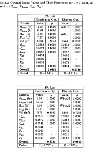
Structural Design under Seismic Risk Using Multiple Performance Objectives

(1)

Using Multiple Performance Objectives

Thesis by

Ayhan Irfanoglu

In Partial Fulfillment of the Requirements for the Degree of

Doctor of Philosophy

California Institute of Technology Pasadena, California

2000

(2)

©

2000

(3)

Acknowledgements

I am deeply thankful to my advisor Prof. James L. Beck for all he has done for me. This study would not have been possible if it were not for him. Our long conversations on practically everything have been most enjoyable.

I truly appreciate the time and input of Professors John F. Hall, Thomas H. Heaton, Wilfred D. Iwan, Paul C. Jennings, and Ronald F. Scott in reviewing my thesis and being on my examination committee. It has been an invaluable experience to be their student, as well. Academicians_ like them, like Prof. Joel N. Franklin, make Caltech what it is: a wonderful institution and a genuine center of excellence and integrity. It is a blessing to have been here.

I am also thankful to Prof. Constantinos Papadimitriou for his support.

My studies were· financially supported by funds from California Universities for Research in Earthquake Engineering under the CUREe-Kajima Joint Research Pro-gram, Phases II and III; Pacific Earthquake Engineering Research Center under NSF Cooperative Agreement No. EEC-9701568; NSF under grant BCS-9309149; and, Harold Hellwig Fellowship in Structural Engineering. These supports and Caltech's support through teaching assistanships are gratefully acknowledged.

I am thankful to Sharon Beckenbach, Denise Okamoto, Raul Relles, Carolina Sus-taita, and Connie Yehle; to Cecilia Lin for always being so thoughtful and supportive; to Leslie Crockett and Philip Roche for their help, sharing, and their contributions to the irfanoglu Library - a dream we have recently realized back at home.

(4)

The great love and support of my Mother and Father, Umran and Mustafa Kemal Irfanoglu, and my brothers, Orhan and Biilent, made me attain this state in life. I am truly thankful to them. God willing, with their backing will I use the experience and knowledge I have acquired at Caltech to help those who are less fortunate.

(5)

Abstract

Structural desigh is a decision-making process in which a wide spectrum of re-quirements, expectations, and concerns needs to be properly addressed. Engineering design criteria are considered together with societal and client preferences, and most of these design objectives are affected by the uncertainties surrounding a design. Therefore, realistic design frameworks must be able to handle multiple performance objectives and incorporate uncertainties from numerous sources into the process.

In this study, a multi-criteria based design framework for structural design under seismic risk is explored. The emphasis is on reliability-based performance objectives and their interaction with economic objectives. The framework has analysis, eval-uation, and revision stages. In the probabilistic response analysis, seismic loading uncertainties as well as modeling uncertainties are incorporated. For evaluation, two approaches are suggested: one based on preference aggregation and the other based on socio-economics. Both implementations of the general framework are illustrated with simple but informative design examples to explore the basic features of the framework.

The first approach uses concepts similar to those found in multi-criteria decision theory, and directly combines reliability-based objectives with others. This approach is implemented in a single-stage design procedure. In the socio-economics based approach, a two-stage design procedure is recommended in which societal preferences are treated through reliability-based engineering performance measures, but emphasis is also given to economic objectives because these are especially important to the structural designer's client. A rational net asset value formulation including losses from uncertain future earthquakes is used to assess the economic performance of a design. A recently developed assembly-based vulnerability analysis is incorporated into the loss estimation.

(6)

(7)

..

_- 103

(9)

Chapter 1 Introduction

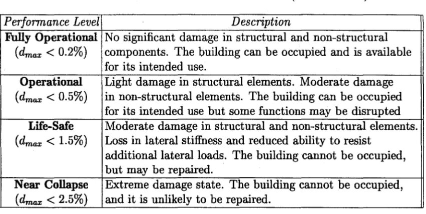
After every destructive earthquake, greater attention is given to the issues as-sociated with structural design. In post-earthquake studies, engineering-based per-formance evaluations often constitute most of the effort. However, especially after recent earthquakes, the performance of structures, both individually and collectively, has been increasingly expressed in terms of non-engineering measures, such as eco-nomic losses. Along with this shift, basic assumptions regarding design objectives have been scrutinized and, as a result, they are receiving heavy criticism. For ex-ample, the design premise that has been in force for decades states that structures designed following code specifications "in general, should resist a minor level of earth-quake ground motion without damage; a moderate level of earthearth-quake ground motion without structural damage, while possibly experiencing some non-structural damage; and, a major level of earthquake motion without collapse, but possibly with some structural and non-structural damage" (SEAOC 1996). This statement is not very clear because the terms used in expressing the objectives are not well-defined. Further-more, there is dissatisfaction with the way design codes implement these objectives because it is felt that only the life-safety condition is explicitly addressed in the codes and that they do not adequately treat the other two objectives stated in the design premise and which focus on damage prevention. The choice of life-safety condition has been dominant because it is the minimum requirement of the code, and quite often, structures are designed just to meet that, and no more. Unfortunately, this condition does not necessarily guarantee that the other two objectives would be met by such a designed structure. However, there are reasons why the first two objectives are generally ignored: no clear definitions of the damage terms or explicit damage prevention measures are given. This is exactly where the new paradigm in structural design has its roots.

(10)

as well as by society, and the codes stop short of converting the engineering design objectives into these economic terms. It is left to the designers to implicitly do the conversion and they often do not have quantitative methods of doing it. However, advances are being made in analytical, computational, and experimental tools in the fields of seismology, earthquake engineering, and economics to fill the gaps. In the meantime, to meet the new higher expectations from clients as well as to address societal concerns, the structural design profession has moved from the vague and qualitative performance objectives to well-defined and quantitative ones (ATC 1995). Professional and governmental organizations, as well as private researchers, have been conducting numerous studies to support this movement.

Vision 2000, a pioneering report prepared by SEAOC (1995), acted as the main

document to initiate development of practical performance-based design methodolo-gies and concepts, and the new attitude has been affecting design practice with re-gard to both existing structures (ATC 1996, 1997a, 1997b) and the new ones (BSSC 1997a, 1997b). The designer can no longer design to meet only the code minimum requirements and claim success. There are now multiple and quantitatively-stated performance objectives to meet.

(11)

et al. 1999a). However, few studies of this kind are implemented to understand the nature of non-engineering based performance of a structure, such as economics based ones (Ang et al. 1996; Ang and De Leon 1997; Beck et al. 1999b, 1999c; Wen 1999) and even fewer consider other non-engineering based performance criteria that might need to be considered during design (Austin et al. 1985; Takewaki et al. 1991; Beck et al. 1996a, 1996b, 1999a).

However, there are still many challenging conceptual and implementational issues to be addressed before recommended performance-based design approaches receive wide approval in practice (Blockley and Elms 1999). For example, do the performance objectives that are generally expressed in terms of reliability or risk levels at various limit-states relate well to client's, as well as society's, preferences? How do they relate to life-cycle costs? Would the performance objective specifications overconstrain the feasible design space and force a resulting design to be a suboptimal one in some sense? And of course, there is the overriding question: how should an optimal or a best design be defined and how would it be implemented in practice?

In this study, an attempt is made to address the challenges of this new envi-ronment, and a formal framework for structural design under multiple performance objectives and in the presence of uncertainties is given. In the framework, reliability-based criteria, and concepts similar to those found in multi-criteria decision theory are used to navigate the uncertain decision-making environment structural designers work in.

(12)

Chapter 2 A Reliability-Based Multi-Criteria

Framework for Structural Design under

Seismic Risk

2.1 Introduction

The design decision-making process is an iterative procedure wherein a prelimi-nary design is cycled through stages of analysis, evaluation, and revision to achieve a design that satisfies various criteria best in some chosen sense. In the design method-ology proposed in this study, a rational model of the decision-making process is made through a formal treatment of these three design stages. The development of the framework was initiated as part of a CUREe-Kajima Phase II project (Beck et al. 1996a, 1997, 1999a). The scope of the framework was extended based on research from CUREe-Kajima Phase III (Beck et al. 1999b, 1999c) and PEER projects (Beck et al. 1999d).

The methodology handles the key aspects of decision-making in a design process in a consistent and formal way. Uncertainties associated with the designed struc-ture and the design process itself are incorporated into the framework explicitly and quantitatively. This incorporation allows a better observation of and insight into the effects of uncertainties on the resulting design. The methodology employs a modu-lar approach to the structural design decision-making process. Therefore, it has the flexibility to allow updates and expansions in specific stages, as well as in an overall sense, as improved models of the design process are developed.

(13)

performance of a structure play an important role in design decisions. A brief overview

of the evaluation stage will introduce two approaches. However, extensive studies of

these approaches are left to later chapters where their use within the framework will

be explained and illustrated by some examples. For the revision stage, only a very

general review will be given since the methods used for revision have been treated in

detail elsewhere, and the emphasis of this study is not on this aspect of the framework.

DESIGN PARAMETERS

• Structural material type • Structural configuration • Member dimensions

ANALYSIS 0 Finite element analysis

Prob. analysis tools

Seismic Loading Uncertainty • Seismic hazard model • Design Loads:

- PSV response spectrum - Stochastic time bisti>ly

PERFORMANCE PARAMETERS

• Design parameters e.g. member dimensions • Structural response parameters

e.g. interstory drift, member stresses • Lifetime reliability

• Costs e.g. construction~ life-cycle

EVALUATION q{0) Aggregation of the design

.,_.._ ... criteria:

- Multiple Criteria based - Socio-Economics based

REVISION 0+o0

[image:13.603.110.483.199.456.2]

Optimization

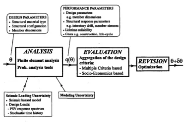
Figure 2.1: Iterative Design Framework for Performance Based Structural Design

Using Fig. 2.1 as an overview, the framework could be summarized as follows.

Structural design starts with a description of the design problem as comprehensive

as possible. The "design parameters" that are to be varied during the design process

need to be specified. These parameters can be, for example, those that specify the

structural configuration or cons~ruction materials to be used, which might be the case

in early stages of the design decision-making process. Or they can be related to the

geometric information for the structural members, such as cross-sectional dimensions

(14)

configuration are chosen. Also, the designer must specify all design requirements, that is, "design criteria," on which each design is to be judged, and list the performance parameters involved in each design criterion. The performance parameters represent quantities related to the "performance" of the design, and can take the form of con-ventional structural parameters (for example, stress, deflection, interstory drift, or modal frequencies) or other parameters (for example, structural reliability, material cost of the structural system, life-cycle cost of the structure). The designer then chooses a structural system configuration as well as the geometrical and connection information for each structural member to obtain a preliminary design. Furthermore, the designer needs to specify all possible loading cases and associated uncertainties ("loading uncertainties") that the structure might experience during its lifetime. The choice of these cases is of utmost importance since the structural design is greatly affected by them. The "loading" module shown in Fig. 2.1 corresponds to the case of structural design against seismic loads, which is the focus of this work. However, any type of loading, with proper specification of its interaction with the designed struc-ture as well as the associated loading uncertainties, could be included in the loading module.

In the first stage of the design process, the performance parameter values un-der the specified loading cases are computed through chosen analysis methods. It is important to realize that, whichever resp~nse analysis method is used (for example, static, response spectrum or dynamic), there will be an uncertainty in the computed results due not only to the uncertainties in the loads applied to the structure but also to the uncertainties related to the modeling of the structure and the analysis method employed (Beck and Katafygiotis 1998). In other words, there will be "mod-eling uncertainties" as well as "loading uncertainties." A rational treatment of these uncertainties and their effects on the design can be carried out by using probabilis-tic models and analysis tools. However, some performance parameters, such as the amount of structural material to be used for the current design, may contain very little uncertainty and so not require any probabilistic structural analysis.

(15)

to judge how well each design criterion is satisfied. This is the evaluation stage. In general, not every criterion will be satisfied in an optimal manner by the preliminary design. Therefore, the designer must revise the initial design in order to obtain a better one by trying to better satisfy the design criteria collectively. However, usually it is not possible to•·maximally satisfy all criteria simultaneously since some of them will conflict with each other. Therefore, a compromise, or trade-off, has to be made when seeking a better design, and an overall design evaluation measure is needed to allow such trading off. This approach to the structural design process converts the issue of structural design into a performance-based multi-criteria optimization problem.

This process of analysis, evaluation and r~vision is repeated iteratively and as long as it is necessary to find a design that is considered to give the best solution to the specified set of design criteria. A detailed study of the methodology developed to solve this problem follows.

2.2 Analysis Stage

In the analysis stage, the design specified by the current values of the design parameters 8 is analyzed to obtain the values of the chosen performance parameters,

q(8). These values will be used in the evaluation stage. The performance parameters are functions of the current design parameters, albeit not always as explicitly as the symbolic expression implies.

(16)

these uncertainties models the state of matters more realistically than those designs ignoring them and therefore yields more accurate and informative results. It is the trade-off between completeness and computational cost that sets the extent of the incorporated uncertainties.

The performance of the structure in such uncertain environments is usually judged by safety considerations, and a measure of safety is provided by component and system reliability. For example, the peak interstory drift over the lifetime of the structure due to earthquakes is uncertain. Thus, a performance parameter that directly relates to the interstory drift reliability can be chosen. Available probabilistic analysis tools are then used to calculate the structural reliability or, equivalently, the failure probability, corresponding to a specified interstory drift limit.

The first step in developing an expression for the probability of structural failure, designated by F(O) for a design with design parameters 8, is to characterize the seismic hazard at the site of the designed structure.

2.2.1 Seismic Hazard Analysis

The objective of a seismic hazard analysis is to obtain a probabilistic description of the ground-motion intensity at the building site over the lifetime of the structure. At a fundamental level, one can express the seismic hazard by a set of ground motion parameters a (for example, response spectrum ordinates, peak ground acceleration, duration of motion, frequency content). For most probabilistic hazard models in use, these parameters depend, through appropriate attenuation relationships, on a set of uncertain seismicity variables 'Y accounting for the uncertain regional seismic environment. For example, 'Y may include variables such as earthquake magnitude, fault dimensions, source parameters, earthquake distance, propagation path proper-ties, and local site conditions. The uncertain values of the seis:rpicity variables 'Y are described by a probability density function p('Y), which is based on seismological studies.

(17)

observed data. There is uncertainty associated with these attenuation models, even when "Y is known, which is reflected by the scatter of the analyzed data about the mean or median model predictions. Therefore, the attenuation relationship should actually give a probabilistic description p(a

I

"Y) of the relation between the ground motion parameters ;a and the seismicity parameters "Y.

In this study, the parameter chosen to represent seismic hazard is Sv, the pseudo-velocity response of the structure corresponding to its fundamental mode, that is, at its elastic fundamental period and selected damping ratio. It is also possible to consider values of Sv corresponding to more than a single mode in a multi-mode re-sponse analysis. However, the fundamental mode in a given direction often dominates the linear response and the contributions of the other modes can be included in the modeling uncertainty. Assuming that a single mode response spectrum analysis is to be used, the task is then to find p(Sv

I

EQ, 8), the probability density function of Sv for the structure represented by 8 given that an uncertain earthquake EQ has oc-curred. Since the earthquake is an uncertain event, a probability distribution over the possible range of event parameters is needed. This can be obtained from a regional seismicity model which represents the seismic environment at the building site. For example, if magnitude M and distance R from the site are chosen as the parameters to represent an earthquake, the formulation for an uncertain event can be given as

p(Sv

I

EQ, 8)

=

r

p(Sv

I

8, M, R) p(M, R

I

EQ) dM dR (2.1)

JM, R

in which p(Sv

I

8, M, R) may be obtained using available ground motion attenuation formulas. The attenuation formula from Boore, Joyner, and Fumal (1993, 1994) is used in this study and is reviewed below.

(18)

p(R

I

EQ)dR is simply the ratio of the area of an annulus of width dR located R distance away from the center to the area of the circle with radius Rmax. The resulting probability density function for the earthquake distance will be

p(R I EQ)

=

2R/ R~ax (2.2)

For modeling the probability distribution of earthquake magnitudes, a truncated form of the Gutenberg-Richter relationship (Gutenberg and Richter 1958; Cornell and Van-marcke 1969) can be used. In this model, the cumulative number of earthquakes per annum with magnitude up to M is given by the relation

(2.3)

where Mmin and Mmax are, respectively, a chosen lower bound and the regional upper

bound for the earthquake magnitude. The expected number of events per annum falling into the magnitude range considered is then given as

(2.4)

where v is also known as the seismicity rate. These relations are consistent with a

Poisson model of the occurrence of earthquakes with mean arrival rate v and each event having a magnitude M distributed according to the probability density function

(2.5)

where b'

=

bloge(lO).

(19)

complex geometries (Cornell 1968; Der Kiureghian and Ang 1977) or choose other parameters to model the seismic environment.

This type of modeling is generally accepted where the seismic sources are spread over a large region and have a large variation in magnitude (''non-characteristic" earthquakes). If there are well-defined sources with a repetitive character around the considered site, uncertain future earthquakes from them could be included as "char-acteristic" events into the seismic environment modeling (for example, Eliopoulos and Wen 1991).

As noted earlier in this study, the seismic hazard from earthquake ground motions is to be characterized by the pseudo-velocity response spectrum Sv(T, ()where Tis the period and (is the damping ratio of a single degree-of-freedom linear oscillator. For the probabilistic seismic hazard model, the attenuation formula proposed by Boore et al. (1993) is used to model Sv(T, ()in terms of earthquake magnitude and distance. This relationship is given as

log10(Sv(T, ())

=

log1o(Sv(T, ())

+

c(T, () (2.6)

where

log10(Sv(T, ()) - ,,,,,..._ bi+~ ... (M - 6) + b3 (M - 6) + ,,,,.... 2 ... b4 r +

bs

log(r)

+

b6

Gb

+

b7

Ge (2.7)

Here, r = .../ R2

+

_h_{2 ,}_where_R_{is the earthquake distance defined as the closest}

hori-zontal distance from the site to the rupture's projection on the earth's surface, and h

(20)

spline fits are obtained for each parameter as a function of the period and the critical damping ratio. A complete description of the variables appearing in the attenuation formula is given in Boore et al. (1993, 1994).

The function c(T, () in Eqn. (2.6) represents the uncertain model error in the ac-tual spectral amplitudes Sv(T, ()compared with the estimated amplitudes Sv(T, ()

from the model. The probability density function for c(T, () is assumed to follow a Gaussian distribution over the range of periods analyzed, with zero mean and variance given in Boore et al. (1994).

To illustrate the use of probabilistic seismic modeling, a comparison of the pseudo-velocity response spectra specified by UBC (ICBO 1994) and the results obtained for a chosen seismic environment using the above formulation are presented. The seismic environment is specified as follows: only those earthquakes within a distance of Rrnax = 50 Km are considered; the surrounding seismic region is not capable of generating earthquakes with magnitudes greater than 7. 7; and it is assumed that earthquakes with magnitudes less than 5.0 have no structural design consequences. Therefore, Mmin

=

5.0 and Mmax

=

7. 7 are chosen. The parameters for the truncated Gutenberg-Richter relationship, Eqn. (2.3), are set as b

=

1.0 and a

=

5.0, which result in a seismicity rate of v

=

1 event/yr in the considered magnitude range. In Fig. 2.2, a qualitative comparison of the seismic hazard in the defined environment and the pseudo-velocity response spectrum specified by UBC (ICBO 1994) for seismic zone 4 (with effective peak ground acceleration of 403 of the gravitational acceleration) and site soil type S2 (medium stiff to stiff soil condition) is given. The response

(21)

type of soil will be assumed which corresponds to site class Bin Boore et al. (1993); it is equivalent to UBC (ICBO 1994) soil type 82). It is observed that, depending on the period range, the UBC spectrum falls between the 4% and 15% exceedance levels of the probabilistic response spectrum for the specified seismic environment.

Similar seismic hazard models with various seismicity rates will be used in the examples in later chapters. It should be noted that, without a model for the proba-bilistic nature of the seismic hazard, no complete analysis of a structural design under seismic risk can be carried out. Therefore, proper specification and modeling of the seismic environment and the hazard it poses to the designed structure are tasks with fundamental importance.

70 ... , ... .

60 . . . "' .. ' ... · .... .

. . ··· _. ... ··· _.

50 _. _.

. . . . . .

: 5%

~-~--~--~--~-:-~--~:..: ~- -~· ~ -~· ~- ~ -~

: 10% 30

20 ... . ... ···.···:.30% : 50% 10 ...

o~~~~~~~~~~~~~~~~~~~~~~~~~

0 0.2 0.4 0.6 0.8 1 1.2 1.4 1.6 1.8 2

Period, T [s]

Figure 2.2: UBC (1994) Response Spectrum for Zone 4, Soil Type S2 , and

Site-Specific Uniform Hazard Spectra for Various Exceedance Probabilities over 50 Years

[image:21.600.113.480.290.590.2]

(22)

2.2.2 Structural Response Analysis

As mentioned above, response spectra are used to express the seismic hazard and, consequently, a pseudo-dynamic type of structural response analysis based on these spectra will be used in this study. However, it has to be emphasized that the theoretical framework can utilize other methods for the response analysis, such as time-history analyses using some form of Monte Carlo simulation (for example, Au, Papadimitriou, and Beck 1999). Whichever response analysis method is chosen, associated tools that treat relevant uncertainties need to be properly developed and incorporated into the framework.

To be able to perform a response spectrum analysis, first of all, a model with discrete lumped masses is formed for the structural configuration. This model includes the concentrated mass and the stiffness values at all considered degrees of freedom. Expressing the mass and stiffness values in matrix form as M and K, respectively, the mathematical formulation for the seismic response becomes

MiC

+

Kx

=

Mfz(t) (2.8)

where

z

is the ground acceleration in the direction of interest, xis the displacement vector for the degrees of freedom of the structural model, and ii! is the associated acceleration vector. In the current study, only the lateral motion in one plane of the structural models is taken into consideration, and therefore the components of influence vector

f

become

Ii

= 1 if i corresponds to a horizontal degree-of-freedom in the plane of interest and

Ii=

0 otherwise. It should be noted that damping need only be specified later when obtaining the relevant response spectral value.

If M and K are Nmx.Nm matrices, the corresponding eigenproblem can be written for each eigenvalue, that is, structural mode, as (Chopra 1995)

(2.9)

(23)

corresponding modal period, </>i is the corresponding mode shape, and Nm is the number of degrees of freedom.

The response of the structure is a superposition of the modal contributions which are found using the corresponding modal frequencies and assumed modal damping ratios. However, to be able to combine these modal responses properly, the corre-sponding modal participation factors need to be computed. For example, the contri-bution to the displacement at the i-th story by the j-th mode, has a peak value diJ given by

(2.10)

where the modal participation factor I'i is given by

(2.11)

if the mass matrix i~ diagonal, M = diag(Mi, ... , MNm).

The peak contributions from each mode can be combined in different ways de-pending on the modal characteristics of the structural system (Der Kiureghian 1981). Structural modeling errors and the uncertainty in an estimate given by the modal combination rule could be included in the analysis. In this study, a single mode analysis based on the response spectra for the fundamental mode of the structure is used.

(24)

2.2.3 Reliability Computations

Knowing the ground motion parameter Sv for a site does not completely specify the structural excitation. Because of the presence of modeling errors, that is, "pa-rameter uncertainties" resulting from incomplete knowledge of the best values of the model parameters to represent the structure together with "prediction-error uncer-tainties" resulting from the imperfect analytical models and analysis methods used in response estimation, the response of the structure cannot be predicted exactly. These uncertainties mean that a failure probability corresponding to a design 8 and conditional on the ground motion parameters, designated by F(8

I

Sv ), must be set up.

In the case of "complete knowledge," that is, if the response of a structure given the Sv value can be predicted precisely, F ( 8

I

Sv) would be a binary function with a value of 0 or 1. Otherwise, the conditional failure probability F(8

I

Sv) can be obtained using probabilistic analysis tools and it will be a function spread over the range between 0 and 1.

F( 8

I

Sv) is also known as the "fragility" of the structure defined by 8 experiencing the seismic attack prescribed by Sv. In a general context, fragilities can be defined at the component or the system levels. Analytic evaluations for component fragilities are possible while the system fragilities are mostly obtained using empirical or simulation techniques.

If the peak interstory drift dmax in a building is taken as an example, the corre-sponding drift risk Fd(8, tu1e) = P(dmax

>

da1zow

I

6, tzite) over the lifetime tzife of the structure can be found as follows. First, the failure probability F(8

I

EQ) given

the occurrence of an earthquake of uncertain magnitude and location, denoted by

EQ, needs to be found. For the peak interstory drift, this can be expressed as

n '

F(8

I

EQ) = P(dmax

>

dallow

I

EQ, 8)

=

P(LJ{di

>

dallow}

I

EQ, 8)

(2.12)

i=l

where n is the number of stories in the building and di is the peak interstory drift in

(25)

The failure probability over the lifetime of the structure is then computed using an occurrence model for earthquake events. Assuming that the occurrences of earth-quakes follow a Poisson arrival process, the probability that the structural safety requirements are not satisfied during the lifetime tiif e years of the structure is given by

Fd(8, t1iJe) = 1 - exp[-v F(8

I

EQ) tliJe] (2.13) where v is the expected number of events per annum, that is, the annual seismicity

rate. How F(8

I

EQ) is computed depends on the modeling assumptions.

If the assumption is made that the interstory drifts, for example, are known

once Sv and 8 are given, the resulting conditional failure probability P( dmax >

dallow

I

Sv, 8) is either 1 or 0, depending ~on whether the safety levels have been

exceeded or not. This is the case for the examples in Chapter 3 where the response uncertainty is ignored. In that case, only Sv is uncertain and the range in the Sv parameter space can be divided into safe and unsafe parts where F ( 8

I

Sv) takes the value 0 or 1, respectively.

First, consider the case of component reliability for which there is a single fail-ure point, typically given in the implicit form g(Sv) = 0, separating the safe and unsafe parts of the parameter space of Sv: S

= {

Sv E R : g ( Sv)

>

O} and :F

=

{Sv ER: g(Sv)

<

O}, respectively. The probability of failure then becomes

F(B

I

EQ) =

1

p(Sv

I

EQ,8)dSv

g(Sv)<O

(2.14)

In this study, a trapezoidal numerical integration scheme in MATLAB (MathWorks Inc. 1998) is used to evaluate Eqn. (2.14). This reliability integral can also be evaluated approximately using available first-order or second-order reliability methods (for example, Madsen et al. 1986; Der Kiureghian et al. 1987; Breitung 1989; Polidori et al. 1999).

(26)

component failure points collectively, the formulation can be made as follows. Let

gi(Sv)

=

0 be the equation for the i-th failure point. The unsafe interval for Sv is

the union of the unsafe ranges for each component. The reliability integral for the failure probability given the occurrence of an earthquake is then

F(8

I

EQ) =

1 .

p(Sv

I

EQ, 8) dSv

ur=l

9i(sv)<o

(2.15)

which is in the form of the classical reliability expression for a series system. This type of reliability is encountered in design when, for example, design criteria specify upper limits on the maximum lifetime drift at each story. The limit point 9i(Sv) = 0 in this case is the interstory drift requirement for the i-th floor so the failure probability is given by Eqn. (2.15) where Yi= 9i(Sv)

=

dallow - di(Sv ).

Simplified approximations to the reliability integral in Eqn. (2.15) can be given in several cases, provided certain conditions apply. One approximation is to replace the reliability integral by the sum of the component reliability integrals, that is, summing the contributions from each component, which works well if the contributions from the overlapping failure ranges are insignificant. Another approximation is, however, to consider the contribution from the component with the highest failure probability while neglecting the contributions from the other components. This will yield a good approximation if the contributions from failures of the other components are insignificant or if the significant parts of the failure ranges of the other components are subsets of the failure range of the component with the highest failure probability. In the numerical results that follow, it is found that considering only the component corresponding to the highest failure probability results in a good approximation of the system reliability for the type of design problem to be discussed therein.

(27)

Au, Papadimitriou, and Beck 1999) or asymptotic methods (Papadimitriou, Beck, and Katafygiotis 1997) need to be used. An example using the asymptotic method for a multi-mode probabilistic analysis can be found in Beck et al. (1997, 1999a).

In Chapter 4, the response uncertainty given Sv is considered at the expense of increased computat.ional effort. In this case, it is explicitly acknowledged that Sv does not define completely the response of a multi-degree-of-freedom system. Using the total probability theorem, the uncertainties in the seismic environment, ground motion modeling and structural modeling can be combined to determine the total failure probability given the occurrence of an earthquake event as

F(8 \ EQ) =iv F(O \

S~)

p(Sv \ EQ, 8) dSv (2.16)

where F(8

I

Sv) = 1-P(dmax :::; dallowl 8, Sv ). The cumulative distribution function

on the drift response can be determined by assuming a log-normal probability distri-bution on the drift given Sv, where the median is given by the fundamental mode response and a proper log-standard deviation is determined by simulations (Shome et al. 1998; Beck et al. 1999c).

2.3 Evaluation Stage: Two Approaches

The objective of the evaluation stage of the optimal design methodology is to obtain an overall design evaluation measure for the design specified by the current value of the design parameters. This measure serves as an objective function which, at the revision stage, is used to determine improved, or optimal, designs.

In general, for evaluation of the design, the designer may wish to impose numerous design criteria. These criteria might be related to structural material choice, element dimension, or overall configuration, and therefore, could be classified as architectural or constructional preferences. They might be related to engineering performance ob-jectives, such as the peak responses of the structure under various types and levels of

(28)

pref-erences related to life-cycle costs, including construction and various life-time costs. Therefore, the problem is fundamentally a multi-criteria decision-making problem in the presence of uncertainties. A methodology is required in which a design can be quantitatively evaluated on the basis of each design criterion individually as well as all of them collectively. Furthermore, since not every design criterion can be satisfied to its maximum extent simultaneously with the other design criteria, the methodol-ogy must allow a trade-off to occur between conflicting criteria in the optimization process. To trade off in a controlled manner, the designer should also be given the freedom to set the relative importance of each design criterion explicitly.

Two approaches to perform the overall evaluation have been developed for the design methodology. The first one, an approach based on multi-criteria decision theory (Keeney and Raiffa 1976; Cohon 1978; French 1988), begins by evaluating each design criterion separately and then combines them in a chosen way to obtain an overall design evaluation measure. The second approach is a socio-economics based one, and treats the problem differently. It converts the consequences of various choices and limit-states into monetary terms. However, it still allows explicit imposition of reliability-based preferences. These two approaches give two different ways to look at the problem of structural design decision-making, and the resulting designs from these approaches would in general be different. This is not due to any inconsistency of the design methodology or the evaluation approaches but is due to lack of explicit transformations between the preferences used or implied in the two approaches. Since these multi-criteria based and socio-economics based approaches will be studied in detail in Chapter 3 and Chapter 4, respectively, only brief introductions to each one are given in here.

(29)

which is believed to be both intuitive and practical will be studied in detail and illustrated with example applications in Chapter 3.

The second approach to be explored is a socio-economics based one. Despite its engineering and therefore technical nature, the design process has to produce results that satisfy qualitative criteria demanded by society, as well as others expected by the client. It needs to be mentioned that modeling the preferences associated with these criteria is often a very challenging task. A simple but informative approach to evaluate the current design based on socio-economic objectives will be explained and illustrated in Chapter 4.

2.4 Revision Stage

Due to the nature of the engineering design processes, the methodology has two interrelated aspects: modeling the structural decision-making process in which mul-tiple objectives can be specified quantitatively, and optimization of these objectives in some sense. In this study, emphasis is given to the former aspect. Therefore, only an overview of the revision stage is given here.

In this stage, the objective is to find the values for the design parameters that maximize the overall design evaluation measure and thus give the optimal design. Convergence to this design takes place in an iterative manner and the rate of con-vergence depends not only on the nature of the problem and the complexity of its mathematical formulation but also on the characteristics of the optimization tech-nique employed. In this study, especially since the multi-objective design process has been transformed into a non-constrained mathematical optimization problem, numerous techniques could be used. However, due to the heavy computational effort required at the analysis stage, especially by structural analyses in the case of large structural systems, and by the probabilistic structural response estimations with high dimensional integral evaluations, the type of optimization techniques are limited in practice.

(30)

In searching for optimal designs the adaptive random search technique is used (Masri et al. 1980). In practice, the design parameters are generally defined over a discrete set. For example, if these parameters are the dimensions of the structural members, say, I-sections, then a discrete set of sizes needs to be considered, such as the W-shapes listed in the AISC manufactured steel I-sections catalogs (AISC 1989). In such cases, even though the results for an optimal design over continuous parameters could be used as an aid, ultimately, discrete optimization methods need to be used. Genetic algorithms are such methods; the use of genetic algorithms in structural optimization and also within the multi-objective design methodology is given in Beck et al. (1997) and Chan (1997). In some of the examples presented later, results obtained from searches over small discrete sets will be used for comparison with the optimal design based on continuous design parameters.

2.5 Concluding Remarks

(31)

Chapter 3 Design Evaluation Using

Preference ,.Aggregation of Multiple

Performance Objectives

3.1 Introduction

(32)

In this chapter, an analytical approach to assist in evaluating the performance of a design is presented. It fits into the evaluation stage of the conceptual framework for structural design based on multiple criteria that was explained in Chapter 2. The approach includes specification of preferences on various design criteria (performance objectives), as well as an aggregation rule that can be used to combine the individual preferences to yield an overall design evaluation measure. The fundamentals of the approach were developed by Beck et al. (1996a, 1996b, 1997). The approach is explained in the next section. Integration of reliability-based objectives into this multi-criteria design framework is emphasized. A simple structure is then designed under various circumstances to illustrate the optimal design methodology. Some comments are made on various performance objectives, especially those required or recommended by the structural engineering design profession, based on the results.

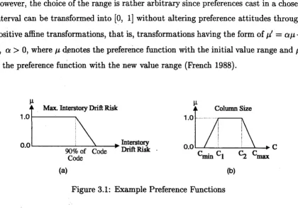
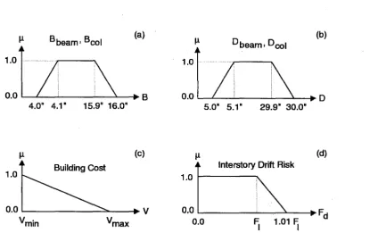
3.2 Preference Functions and Preference Aggregation

In order to perform a quantitative evaluation of a design, a set of preference func-tions µi, i = 1, ... , Ne corresponding to Ne design criteria is specified where µi defines the preference for the various values of each design parameter or performance param-eter involved in the corresponding criterion. Within the current context, a preference function is a value function that may simply express a minimum and/or maximum fuzzy bound on a design quantity (design parameter or performance parameter), or it may express a more complex design criterion (such as a function of various de-sign quantities). For a given performance parameter value, a larger preference value at one performance parameter value compared to that for another performance pa-rameter value implies that the decision-maker prefers the first papa-rameter value more than the other. An equivalence of preference values implies an indifference of the decision-maker between the corresponding values of the performance parameter. In other words, a preference function is an ordinal value function that ranks the values of the respective performance parameter using the associated preference values.

(33)

function can take must lie in a standard range, for example, the unit interval

[O,

1]. However, the choice of the range is rather arbitrary since preferences cast in a chosen interval can be transformed into (0, 1] without altering preference attitudes through positive affine transformations, that is, transformations having the form ofµ' = aµ+

/3,

a>

0, whereµ denotes the preference function with the initial value range andµ' is the preference function with the new value range (French 1988).

µ

Max. Interstoi:y Drift Risk µ Column Size

1.01---~ _1.0

o o . _

__._ _ __._ _ _

Interstoi:y

· 90% of Code Drift Risk Code

o.o~~--~---c

Cmin Cl C2 Cmax

[image:33.593.83.503.76.370.2]

(a) (b)

Figure 3.1: Example Preference Functions

(34)

parameter. Such discontinuous preferences are believed to be unrealistic in many engineering designs. Almost always, there exists a fuzzy tolerance region between the totally satisfactory and totally unsatisfactory performance parameter values. Besides, in many cases, the performance parameter involved has associated uncertainty and is not as crisp to justify hard boundaries. In other words, the value obtained from an analysis for that performance parameter is not certain, and rejecting or accepting a design due to some small variations in that parameter can not be justified. Therefore, fuzzy transitions ("soft" boundaries) are recommended for use at the regions where a performance criterion changes from acceptable to unacceptable.

In the current approach, constraints directly imposed on the design parameters, such as geometrical and/or material constraints, are treated as additional design cri-teria. By treating design parameter constraints in this way, the degree to which the constraint is satisfied can be traded off against other design criteria during the optimization of the design if a preference function is used to express it as a "soft" constraint. Of course, "hard" constraints do not allow trade-off as they are either satisfied or not satisfied and accept no compromise. For example, a preference func-tion similar to the one shown in Fig. 3.l(a) can be used to express a "soft" upper bound on a design parameter. If the designer also wishes to impose a lower bound on the parameter, then a two-sided version of the preference function can be used. For example, if one chooses column sizes as one of the design parameters, upper and lower limits might need to be imposed on them. This might be due to architectural requirements or simply because of limited availability of member sizes. A possible preference function for such a design criterion is given in Fig. 3.l(b). Various prefer-ence functions will be utilized in the examples later in this chapter (see Figs. 3.3 and 3.4).

(35)

with the design. Another interpretation is to view the preference function as a mem-bership function for the fuzzy set of "acceptable performance" as judged by the i-th design criterion. In this case, an extreme value µi(q(8))

=

1, or µi(q(8))

=

0, im-plies that on the basis of the i-th design criterion, the current design specified by 8

is definitely acceptable, or definitely unacceptable, respectively. Intermediate values express the degree of performance acceptance given by the design. In this sense, preference functions act as the "weak ordering" functions (French 1988). There are other ways to specify the performance preferences. One example is the approach which uses functions that are complements of the preference functions defined above, namely "dissatisfaction functions" (Austin et al. 1985; Takewaki et al. 1991). As long as certain mathematical requirements for preference ordering and value functions are met, any expression of performance preferences could be used, and the choice be-comes a question of convenience and ease of use. The mathematical properties that need to be satisfied to qualify as acceptable preference functions are rather involved, but can be broken into transitivity, negative transitivity, symmetry, antisymmetry, reflexivity, and comparability. The reader is referred to French (1988) for a detailed treatment of these requirements.

It should be noted that the fundamental assumption that allows specification of preference functions is that the decision-maker can assign preferences to the values of the corresponding performance parameters. Of course, this requires that the per-formance parameters be tangible, that is, that they could be measured or assigned a value on some scale. As a result, once the decision-maker breaks the complex perfor-mance objectives space into individual objectives, the objectives can be expressed as preferences over the corresponding performance parameter values.

(36)

approaches demonstrated using a simple design problem).

A preference aggregation rule is simply a functional relationship,

f,

between the individual preference values, µ1 , µ2 , •.. , µNe for all of the design criteria and the overall design evaluation measure, µ (Keeney and Raiffa 1976). An optimal design for a given preference aggregation rule is therefore given by a design parameter vector

8 that maximizes

(3.1)

where it is understood that some of the preference functions µi may correspond to design parameter constraints and, therefore, depend directly on the design parameter values while the rest are functions of performance parameters which are not necessarily analytical functions of the design parameters but nevertheless can be computed, say, through structural response analyses.

By incorporating the design criteria (including design constraints) through the preference aggregation rule into the objective function (the overall design evaluation measure), which is to be maximized by varying the design parameters, the constrained optimization problem is converted into an unconstrained optimization problem.

Axioms of consistency imposed on the preference aggregation rule are (Otto 1992; Scott 1999):

1. The overall design evaluation measure µ lies in the unit interval

[O,

1), with µ

=

1 for a perfectly acceptable design and µ

=

0 for a completely unacceptable design. As mentioned above, this requirement is for the sake of consistency, and the value range could be rearranged.

(37)

small change in the preference for a design based on any of the design criteria produces only a corresponding small change inµ.

3. Symmetry: µ

=

f(µ1, ... , µi, µi+l, ... )

=

f(µ1, ... , µi+i, µi, ... ), that is, the aggregation rule should be symmetric with respect to pairs of individual preference functions and their associated importance weights.

4. Idem potency: µ0

=

f

(µ0 , µo, ... , µ0 ), that is, if the individual preferences for a design based on each criterion have the same value, then the overall preference for the design must have this value.

5. Annihilation: µ = 0 if and only if µi = 0 for some i. That is, a design is completely unacceptable in the overall sense if and only if it is completely un-acceptable on the basis of at least one design criterion.

To be able to combine the multiple design criteria in a preferred manner to obtain a measure for the overall rating of the design, the designer must also specify importance weights, Wi, i = 1, ... , Ne with Wi ;::: 0, which indicate the relative importance of each of the design criteria. Thus, increasing the value of an importance weight for a design criterion gives it more influence in the trade-off that occurs between the various conflicting criteria during optimization of the design. This should hold true irrespective of the rule chosen to combine the multiple design criteria.

(38)

• Conservative ("weakest link," "non-compensating") strategy:

(3.2)

where ni

=

wifwmax, i

=

1, ... , Ne., Wi is a positive importance weight assigned

to the i-th design criterion and Wmax is the maximum of Wi over i = 1, ... , Ne.

• Multiplicative trade-off strategy:

µ _ µ miµ m2 µ mNc

- 1 2 · · · Ne (3.3)

where mi

=

wi/'L,f:,

₁

w;,

i

=

1, ... , Ne, and Wi is a positive importance weight

assigned to the i-th design criterion.

AB already described, the importance weight assigned to each design criterion can be used to control its trade-off relative to the other criteria. That is, selected design criteria can be given more influence than others during optimization by as-signing larger values to their importance weights. The choice of the values for these weights is subjective. The designer/decision-maker is presumed to develop insight with respect to their selection in any design problem by investigating the influence of different values of the weights on the final optimal design and on the correspond-ing preference values for each design crit.erion. For example, if the designer wishes to perform an "aggressive" code-based design that approaches close to the code drift limit (Fig. 3.l(a)), the importance weight for a building cost criterion, which will con-flict with the code drift criterion, should be made much larger than the importance weights for the other design criteria. This will give greater emphasis on reducing costs during the trade-off in the optimization at the expense of giving a design that is much closer to the code drift limit. However, this interaction depends very much

"

on the corresponding preference functions and the aggregation rule used to combine them.

The importance weights wi can be viewed from another perspective. Since there

(39)

be able to independently control their influence during the trade-off that occurs in the optimization process. In the case that the Wi are all equal, the trade-off is governed by the inherent sensitivity of each µi with respect to 0. This "natural" trade-off may

not satisfy the designer, who may want to give greater influence to selected criteria. In this case, an importance weight, say Wj, can be increased, then the sensitivity of µi with respect to 0 will be increased, which will give the j-th criterion more influence

during the optimization. As an aside, it should be noted that a sensitivity study of the decision outcome in relation to individual criterion is the primary tool in reducing the dimension of the relevant performance parameter space. Those parameters to which the design is not sensitive may be taken out of the performance parameter list without compromising the final decision outcome. However, some of the parameters might require monitoring as they might be associated with some constraints that need to be satisfied but are expressed in the form of "hard" constraints and therefore might be mistaken as being irrelevant.

Unfortunately, in most practical problems, a sensitivity study can be done only numerically or empirically even though the underlying concept is simple. For a some-what different but relevant and important stage of the design decision-making process, namely, the "negotiation" stage, there have been some attempts to analytically study the implications of sensitivities (Scott 1999). The relevance of "negotiation" to the structural design process should be clear when one realizes that the decision-makers in structural design do not necessarily have a unique common interest or employ similar approaches in evaluating the design. This is especially true in the multiple criteria based approaches where the criteria and preferences need to be stated explicitly.

(40)

Eqn. (3.3) is used in the examples presented later in this chapter.

Before illustrating the methodology with examples, it should be noted that special cases of the optimal design methodology based on the multiplicative trade-off strategy can be related to existing optimal design concepts. For example, it is easily shown that the optimal solution obtained by maximizing Eqn. (3.3) belongs to the Pareto optimal set corresponding to the multiple "objectives" µ1 , ... , µNe (Chan 1997). But in contrast to an approach based on the full Pareto optimal set, which is not feasible for most practical problems due to the size of the set, the current approach converges to a Pareto optimal design directly. Often, finding one such optimal design is enough.

3.3 Illustrative Design Example: Three-Story SMRF,

Case 1

3.3.1 Structural Model, Design Criteria, and Seismic Environment

Model

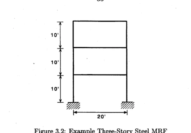
The optimal multi-criteria design methodology using the multiplicative trade-off strategy is demonstrated by applying it to the design of a three-story, single-bay moment-resisting steel frame. The frame members are all taken as I-sections made out of ASTM A36 (Fy

=

36 ksi) steel with the length of the floor beams fixed at 20

ft and the height of the story columns fixed at 10 ft. The connections are modeled as being rigid and the steel sections are used in their strong axes. Gravity loads are taken as the sum of 60 lb/ft2 _{and 50 lb/ft}2

, from the dead and live loads, respectively,

for each floor and the roof. An out-of-plane tributary width of 100 inches is used for the gravity load calculations. The gravity loads are assumed to participate in the lateral seismic loading in full.

(41)

1 O'

1

o·

[image:41.595.121.453.39.270.2]

20'

Figure 3.2: Example Three-Story Steel MRF

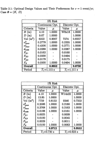
8

=

(B, D), where the beams and columns are required to have the same cross-sectional dimensions, and (b) 8 = (Bbeami Dbeami Ecol, Dc01), where the beams and

columns are allowedto have different cross-sectional dimensions. The flange and web plate thicknesses are held fixed at 0.25 inches. In the continuous case, the adaptive random search algorithm (Masri et al. 1980) is used to obtain the optimal design. The simplicity of the designs allowed search over a small set of relevant AISC W-shapes (AISC 1989) for discrete optimization and an exhaustive search is performed.

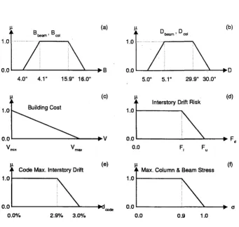
The objective is to determine the best combination of values for the design param-eters 8 so that the frame design is optimized according to design criteria involving the following performance parameters: (a) flange width, (b) web depth, (c) building cost, (d) probability of unacceptable peak lifetime interstory drift (drift risk), and (e) code-based maximum interstory drift and ( e) maximum allowable stresses in struc-tural members (see Fig. 3.3). The importance weight for each design criterion is set to 1.0 for the aggregation of preference values in equation Eqn. (3.3), unless otherwise stated. The corresponding preference functions are shown in Fig. 3.3.

(42)

(a) (b)

.. B 1110

4.0" 4.1" 15.9" 16.0" 5.0" 5.1" 29.9" 30.0"

(c)

lnterstory Drift Risk

(d)

1.0 Building Cost 1.0 1---...

0.0 v 0.0 _Fd

vmin vmax 0.0 F, Fu

I!-Code Max. lnterstory Drift

(e)

I!-Max. Column & Beam Stress (t)

1.0 1.0

0.0 ,__ _ _ _ _ ...._ _ _.__--.Ocode

0.0 - - - CJ

[image:42.583.106.447.62.385.2]

0.0% 2.9% 3.0% 0.0 0.9 1.0

Figure 3.3: Preference Functions for Different Performance Parameters

preference functions show that, for example, in the case of flange width B, members with flange widths shorter than 4.0 inches or longer than 16.0 inches are unacceptable, and therefore are assigned µ values of 0, while those with flange widths between 4.1 to 15.9 inches are favored the most, and therefore are assignedµ values of 1. Flange widths between 4 to 4.1 inches and 15.9 to 16.0 inches have various intermediate de-grees of acceptance or satisfaction. One can interpret the preference function for the web depth D of the structural members in a similar way. In real-life applications, the

(43)

and directly incorporated in the multiplicative trade-off preference aggregation rule given in Eqn. (3.3).

The preference function for the building cost is given in Fig. 3.3( c). For this example, the building cost C is expressed simply as the sum of a construction (or fabrication) cost Gean and a material cost

C

=

Ccon +Cs V (3.4)

where cs is the material cost per unit steel volume and V is the volume of steel used in the design. The variation in the construction costs for structural members of different sizes is assumed negligibly small, so that Ccon is taken to be essentially

independent of (J. The preference function can then be expressed in terms of a

normalized performance parameter

qcost

=

(C - Cmin) / (Cmax - Cmin)

=

(V - Vmin) / (Vmax - Vmin) (3.5)

where Vmax=22,140 in3 and Vmin=4,500 in3 _{are the steel volumes corresponding to} use of the maximum and minimum allowable member section sizes prescribed by the geometric constraints. The preference function for the building cost can therefore be expressed in terms of the steel volume V(O) for a design given by 8. As shown in Fig. 3.3( c), a linearly decreasing function is used to specify the preference values for the building cost in terms of the steel volume, with µ = 1 at the minimum allowable volume and µ = 0 at the maximum allowable volume. In the tables of results presented later, the building cost is reported as the volume of steel, V.

(44)

1994) and employing standard fundamental-mode modal analysis. As it can be seen from Fig. 3.3(e), a computed interstory drift ratio lower than 2.93 is considered per-fectly acceptable, while one higher than 33 is considered completely unacceptable. In Fig. 3.3(f), the preference functions for maximum allowable column and beam nor-malized stresses are given. The performance parameter a in this figure is the ratio of

the maximum induced stress to the allowable stress specified in the AISC Manual of Steel Construction (AISC 1989). Stress calculations are carried out considering the end-of-element stresses resulting from combined axial and bending loads due to full gravity and lateral loadings as given in AISC Allowable Stress Design Manual (AISC 1989). Resulting stresses less than 90% of the code-allowable values are considered perfectly acceptable while those greater than the code-allowables are considered com-pletely unacceptable. It should be noted that in practice other stress checks may need to be performed but these are in this simple illustrative example.

The difference between lifetime interstory drift risk and code-based interstory drift is that the former one gives the failure probability of the structure by considering the uncertainties in future loadings using a site-specific seismic environment explicitly, while the code-based calculations consider the deterministic response spectrum spec-ified in the code. The explicit consideration of the failure probability is of great importance in the design process since it provides flexibility in specifying preferences on the reliability of the structure. However, the code-based requirements can be explicitly included in the design criteria to ensure that the legal requirements are satisfied by the resulting design.

Unacceptable drift performance or "failure" occurs if the maximum interstory drift ratio dma:x exceeds a specified allowable drift ratio da11ow = 3% over the lifetime of the structure. The performance parameter is taken as the interstory drift risk, Fd, which

is simply equal to the probability of exceeding dauow over the lifetime of the structure. As shown in Fig. 3.3(d), the interstory drift risk Fd is required to be less than a limit

Structural Design under Seismic Risk Using Multiple Performance Objectives

Using Multiple Performance Objectives

Ayhan Irfanoglu

©

Acknowledgements

Abstract

Contents

..

Chapter 1 Introduction

Chapter 2 A Reliability-Based Multi-Criteria

Framework for Structural Design under

Seismic Risk

2.1 Introduction

2.2

Analysis Stage

2.2.1 Seismic Hazard Analysis

I

I

I

=

r

I

I

I

I

=

=

=

+

bs

+

b6

+

b7

+

=

=

=

=

=

~-~--~--~--~-:-~--~:..: ~- -~· ~ -~· ~- ~ -~

2.2.2 Structural Response Analysis

+

=

z

f

Ii

Ii=

2.2.3 Reliability Computations

I

I

I

I

>

I

I

I

>

I

=

>

I

(2.12)

I

I

I

I

= {

>

=

<

I

1

I

=

I

1 .

I

ur=l

=

o o . _