Technical note: Combining quantile forecasts and predictive distributions of streamflows

https://doi.org/10.5194/hess-21-5493-2017 © Author(s) 2017. This work is distributed under the Creative Commons Attribution 3.0 License.

Technical note: Combining quantile forecasts and predictive

distributions of streamflows

Konrad Bogner, Katharina Liechti, and Massimiliano Zappa

Swiss Federal Institute for Forest, Snow and Landscape Research WSL, Birmensdorf, Switzerland Correspondence to:Konrad Bogner ([email protected])

Received: 17 May 2017 – Discussion started: 29 May 2017

Revised: 26 September 2017 – Accepted: 4 October 2017 – Published: 8 November 2017

Abstract. The enhanced availability of many different hydro-meteorological modelling and forecasting systems raises the issue of how to optimally combine this great deal of information. Especially the usage of deterministic and probabilistic forecasts with sometimes widely divergent pre-dicted future streamflow values makes it even more com-plicated for decision makers to sift out the relevant infor-mation. In this study multiple streamflow forecast informa-tion will be aggregated based on several different predictive distributions, and quantile forecasts. For this combination the Bayesian model averaging (BMA) approach, the non-homogeneous Gaussian regression (NGR), also known as the ensemble model output statistic (EMOS) techniques, and a novel method called Beta-transformed linear pooling (BLP) will be applied. By the help of the quantile score (QS) and the continuous ranked probability score (CRPS), the combi-nation results for the Sihl River in Switzerland with about 5 years of forecast data will be compared and the differ-ences between the raw and optimally combined forecasts will be highlighted. The results demonstrate the importance of applying proper forecast combination methods for decision makers in the field of flood and water resource management.

1 Introduction

The combination, or aggregation, of differing probability dis-tributions into a single one could result in beneficial effects, since the differences between various forecast systems pro-vide a better understanding of the uncertainty about the target quantities, and the aggregates may reflect more accurately the information. However, the biggest advantage of

aggre-gation is that the forecaster is not forced to decide a priori which forecast system is the most reliable at the actual point of issuing a forecast, because the combination method will be optimized at each forecast run by taking into consider-ation the quality of the forecast from previous time steps. Thus, the data themselves will automatically lead to the op-timal decision incorporating all available information about the different deficiencies and strengths of the individual fore-cast systems.

In econometrics and related disciplines, the combination of forecasts has a long tradition starting with Bates and Granger (1969) suggesting the use of empirical weights de-rived from “out of sample” forecast variances. An overview of the last 40 years of forecast combination in the field of economics can be found in Wallis (2011). Thompson (1977) was one of the first who outlined the advantages of forecast combinations in meteorology and Shamseldin et al. (1997) showed different methods of combining the output of ferent hydrological models. In Abrahart and See (2002) dif-ferent combination methods for hydrological forecast mod-els are compared. Diks and Vrugt (2010) compare differ-ent model averaging approaches, showing that a simple re-gression method could result in improvements comparable to more sophisticated methods.

applied in the field of ensemble forecast calibration (Raftery et al., 2005; Fraley et al., 2010) and for flood forecasting purposes, e.g. in Ajami et al. (2007), Vrugt and Robinson (2007), Todini (2008), and Hemri et al. (2013).

In Gneiting et al. (2005) and Gneiting et al. (2007) the term “calibration” is used to describe the statistical consistency between the distributional forecasts and the observations and is a joint property of the predictions and the events that ma-terialize. A state of the art calibration and bias correction method is non-homogeneous Gaussian regression (NGR), also known as the ensemble model output statistic (EMOS) technique of Gneiting et al. (2005). It fits a single parametric predictive probability density function (pdf) using summary statistics from the (multi-model) ensemble and corrects si-multaneously for biases and dispersion errors. Also, NGR has been applied many times successfully for calibrating and combining hydro-meteorological ensemble forecasts (see for example Hemri et al., 2014).

The Beta-transformed linear pooling (BLP) approach, which has been developed recently by Ranjan and Gneiting (2010) and Gneiting and Ranjan (2013) for combining pre-dictive distributions, will be tested and compared with the NGR and the BMA in this study. To the author’s knowledge the BLP and the associated estimation of weights, which as-sign relative importance to the individual predictive distribu-tions, have not been applied to hydrological forecasts so far.

Before the combination methods are applied, the errors of the hydrological model are corrected in order to minimize the difference between the last available observation and the predictions at the time of initialization of the forecast. This process of error correction is later on called post-processing, since it starts after completing the hydrological simulations and predictions given meteorological observations or fore-casts. Depending on the post-processing method, quantiles or pdfs for future streamflows will be derived for each single forecast time step. Whereas quantile regression (QR) meth-ods (Koenker, 2005) and modifications of them will lead to predictions of quantiles, a predictive pdf can be derived for example by the recently developed waveVARX method (Bogner and Pappenberger, 2011) directly. For more details of these post-processing methods, the reader is referred to Bogner et al. (2016), whereas the objective of this paper will be the analysis of combination methods of forecasts. In the next section the three combination methods and the applied verification measures will be described. After the presenta-tion of the data and the results, the outcome of the compari-son will be discussed and summarized in the conclusions.

2 Methods

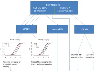
Three different combination methods have been applied to the flood forecasting system for the Sihl River at station Zurich (Switzerland), where two meteorological forecasts, the 16-member COSMO-LEPS (Montani et al., 2011) and

the deterministic C7 system (produced at MeteoSwiss with

≈7 km resolution) are implemented (a detailed description can be found in Addor et al., 2011, Ronco et al., 2015, and Liechti et al., 2016).

In a first step the hydrological modelling errors of all these forecasts will be minimized, using a QR method in com-bination with neural networks (QRNN, Taylor, 2000; Can-non, 2011). This will result in direct estimates of the in-verse cumulative density function (i.e. the quantile function), which in turn allows the derivation of the predictive uncer-tainty (see for example Weerts et al., 2011, López López et al., 2014, and Dogulu et al., 2015, where the applica-tion of the QR in order to estimate predictive uncertain-ties (PUs) is outlined). If the number of estimated quantiles within the domain {0< τ <1}is sufficiently large, the re-sulting distribution could be considered to be continuous. In this study the number of quantiles is set to nine with probabil-ity levelsτ =0.01,0.1,0.2,0.25,0.5,0.75,0.8,0.9,0.99. In Quiñonero Candela et al. (2006) the cdf or pdf is constructed by combining step interpolation of probability densities for specifiedτ-quantiles with exponential lower and upper tails, which will be called the empirical method (EMP). Alterna-tively the pdf could be constructed by monotone re-arranging of theτ-quantiles and estimating a log-normal distribution (LN) to these quantiles for each lead time1t. The advantage of the quantile re-arranging and the distribution fitting is 2-fold and efficiently prevents known problems occurring with QR: firstly it eliminates the problem of crossing of differ-ent quantiles (i.e. the unrealistic but possible outcome of the non-linear optimization problem yielding lower quantiles for higher streamflow values – Chernozhukov et al., 2010 – e.g. the value of the 0.90 quantile is higher than the value of the 0.95 quantile), and secondly it permits the extrapolation to extremes not included in the training sample (Bowden et al., 2012).

This QRNN method will be applied to each ensemble member of the COSMO-LEPS forecasts, resulting in 16 fore-casts of quantiles, and to the C7 forefore-casts. Lichtendahl et al. (2013) have examined averaging quantiles of continuous dis-tributions given by multiple information sources rather than averaging probabilities. Both approaches of probability and quantile averaging have been applied in this paper for aver-aging the post-processed ensemble prediction system (EPS) based streamflow forecasts in order to get one predictive pdf or quantile forecast. Before applying the probability av-eraging approach, a pdf has been constructed by the LN method, i.e. a log-normal distribution has been fitted to the re-arrangedτ-quantiles.

be included in the following combination procedures as well (see Fig. 1).

Three different methods will be tested for optimally com-bining these six forecast models (M1, . . ., M6), which al-low us to assign different weights to the raw and five post-processed forecasts. For the application of the first two meth-ods, BMA and NGR, the streamflow values have been trans-formed to the normal space by the help of the normal quantile transformation (Van der Waerden, 1952, 1953a, b).

2.1 Bayesian model averaging (BMA)

If the combination is calculated within a Bayesian framework by using weights corresponding to the posterior model prob-abilities, it is usually referred to as BMA and follows from direct application of Bayes’ theorem as explained in e.g. Min and Zellner (1993) and Raftery et al. (1997).

In Raftery et al. (2005) the statistical BMA model is ex-tended to dynamical forecast models, where each forecast and/or ensemble member is represented by a probabilistic distribution for which a weight is assigned based on the past performance of each individual forecast. These weights are used to combine all distributions into one single mixture dis-tribution. Therefore the BMA predictive model of the quan-tity of interestyis given by

p(y|k1, . . ., kM)=

M

X

m=1

hmgm(y|km), (1)

where hm is the posterior probability (i.e. weight) of

fore-cast km, the best forecast derived from its performance in

the training period, and the conditional pdf of y on km,

gm(y|km), given thatkmis the best forecast in the ensemble

withm=1, . . ., Mmembers, or models. The transformation

of the streamflow values to the normal space beforehand al-lows the application of the BMA method based on mixtures of univariate normal distributions. In the work of Wang et al. (2012) and Schepen and Wang (2015) variants of the BMA method have been applied, which allow the direct usage of the cdfs for estimating the weighting parameters. However, in this study these BMA approaches have not been imple-mented, and the estimated medians (τ =0.5) from the five post-processing methods and from the raw COSMO-LEPS are taken as input only in order to allow better comparison with the following NGR approach.

2.2 Non-homogeneous Gaussian regression (NGR)

Another possibility to address underdispersion and forecast bias is the use of the NGR method, also known as EMOS, and is based on multiple linear regression for linear vari-ables, such as temperature or streamflows, and logistic re-gression for binary variables, such as precipitation occur-rence or freezing. More information about the MOS tech-nique can be found for example in Glahn and Lowry (1972) and Wilks (1995). Its extension for ensembles is explained

in Gneiting et al. (2005) and a brief summary of this method is given hereafter. Lety denote again the variable of inter-est (e.g. streamflow) and letk1, . . ., kM be the corresponding

forecast of theMensemble members or models. IfN(µ, σ2)

denotes a Gaussian density with meanµand varianceσ2, the NGR predictive distribution is given by

y|k1, . . ., kM ∼N(a0+a1k1+ · · · +aMkM, b0+b1s2),

wheres2= 1

M

M

X

m=1

km−

1

M

M

X

m=1

km

!2

. (2)

Thus the predictive mean is equal to the regression es-timates with coefficients a0, . . ., am, b0, and b1 and forms

a bias-corrected weighted average of the different forecasts (ensemble members), whereas the predictive variance de-pends linearly on the variance of the forecast models (en-semble members). Although modifications for the NGR exist for non-normal distributed variates (see for example Baran, 2014; Baran and Lerch, 2015), the streamflow values have been transformed to the normal space for comparison rea-sons and the medians (τ =0.5) from the five post-processing methods and from the raw COSMO-LEPS are taken as input as in the BMA method.

2.3 Beta-transformed linear pool (BLP)

In Ranjan and Gneiting (2010) it has been stated that any non-trivially weighted average of distinct probability fore-casts will be uncalibrated and lack sharpness, even when the individual forecasts have been calibrated. Hence they sug-gested a composite of the traditional linear pool with a beta transform. The aggregation method introduced by Ranjan and Gneiting (2010) and Gneiting and Ranjan (2013) con-siders the BLP for a set of predictive cdfsF1, . . ., FM as

F (y)=Bα,β

M

X

m=1

ωmFm(y)

!

(3)

fory∈R, whereBα,β denotes the cdf of the standard Beta

distribution with parametersα >0 andβ >0 andω1, . . ., ωM

are non-negative weights that sum to 1. The BLP density forecast for the component densitiesfi, . . ., fM then is

f (y)=

M

X

m=1

ωmfm(y)

!

bα,β

M

X

m=1

ωmFm(y)

!

, (4)

with parametersα >0 andβ >0 of the Beta density function

bα,β. For α=β=1 the BLP corresponds to the traditional

linear opinion pool.

ThusBα,β can be interpreted as a parametric calibration

function for combining F1, . . ., FM with mixture weights

ω∈1M, which assign relative importance to the

Figure 1.Set of six different forecast models available for combination, five post-processed plus one raw forecast. For the quantile averag-ing (M1) and the probability averagaverag-ing (M2) method, an example of averagaverag-ing two ensemble members is indicated.

likelihood method. The log-likelihood function for the BLP model (Eq. 4) is

`(ω1, . . ., ωM;α, β)

=

J

X

j=1

log(f (yj))

=

J

X

j=1

log

M

X

m=1

ωmfmj yj

!

+

J

X

j=1

log bα,β M

X

m=1

ωmFmj yj

!!

(5)

=

J

X

j=1

log

M

X

m=1

ωmfmj yj

!

+

J

X

j=1

(α−1)log

M

X

m=1

ωmFmj yj

!

+(β−1)log 1−

M

X

m=1

ωmFmj yj

!!

+JlogB(α, β)

whereBis the classical Beta function.

This BLP approach has been applied now to combine the different forecast systems. The quantiles resulting from the QRNN method (models M1, M4, and M5) forecasts have

been converted to pdfs by applying the LN method (by fit-ting a log-normal distribution to the re-arrangedτquantiles). 2.4 Verification

Although probability and quantile forecasts are both proba-bilistic products, the former is expressed in terms of a prob-ability (e.g. that a certain threshold will be exceeded) and the latter is given by a quantile for a particular probability level of interest (Bouallègue et al., 2015). Since the outputs of the QRNN model are quantiles, it is reasonable to evalu-ate the performance with a skill score which has been devel-oped for predictive quantiles (Koenker and Machado, 1999; Friederichs and Hense, 2007), known as the quantile score (QS). It is based on an asymmetric piecewise linear func-tion, the so-called check funcfunc-tion,ρτ yi−qτ,i

, which is a function of the probability levelτ (0< τ <1)and the error between the observationyi and the quantile forecastqτ,i for

i=1, . . ., N, whereN is the sample size. The check function

is defined as

ρτ yi−qτ,i=

τ yi−qτ,i ∀yi≥qτ,i

(τ−1) yi−qτ,i ∀yi< qτ,i (6)

Bouallègue et al., 2015): QS=1−τ

N X

i:yi<qτ,i

(qτ,i−yi)+

τ N

X

i:yi≥qτ,i

(yi−qτ,i). (7)

The CRPS compares the forecast probability distribution with the observation and both are represented as cdfs. IfF is the predictive cdf andy is the verifying observation, Gneit-ing and Ranjan (2011) showed that the CRPS can be defined equivalently as a standard form,

CRPS(F, y)=

∞

Z

−∞

(F (t )−I{y≤t})2dt,and as (8)

=2

1 Z

0

Iny < F−1(τ )o−τ F−1(τ )−ydτ. (9)

Thus, in the standard form (Eq. 8) an ensemble of pre-dictions can be converted into a piecewise constant cdf with jumps at the different models (ensemble members), andI{.}

is a Heaviside step function, with a single step from 0 to 1 at the observed value of the variable. The equivalence of Eqs. (8)–(9) was noted by Laio and Tamea (2007). For the quantile forecast qτ=F−1(τ ), the integrand in Eq. (9)

equals the quantile score, i.e. the mean of the check function (Eq. 6). That means the CRPS corresponds to the integral of the QS over all thresholds, or likewise the integral of the QS over all probability levels (Laio and Tamea, 2007 and Gneit-ing and Ranjan, 2011). Hence, the CRPS averages over the complete range of forecast thresholds and probability levels, whereas the QS looks at specificτ-quantiles; thus, it is more efficient in revealing deficiencies in different parts of the dis-tributions, especially with respect to the tails of the distri-bution. Both verification measures are negatively oriented, meaning the smaller the better.

3 Results

COSMO-LEPS and C7 forecasts are available from 24 February 2010 to 27 April 2016 once a day with hourly time resolution, which have been post-processed in order to derive predictive distributions and quantile forecasts. To cal-ibrate and validate the post-processing parameters (QRNN and waveVARX), the data sets of available hourly obser-vations and corresponding simulations have been split into two halves (calibration period: 2010–2012; validation pe-riod: 2013–2016). The results of the validation, which are not shown due to lack of space, highlight the improvements of the QRNN method (similar to the results shown in Bogner et al., 2016).

The weighting parameters of the combination methods are estimated by applying a moving window with a size of 7 days (168 h) for optimization. Different window sizes have been

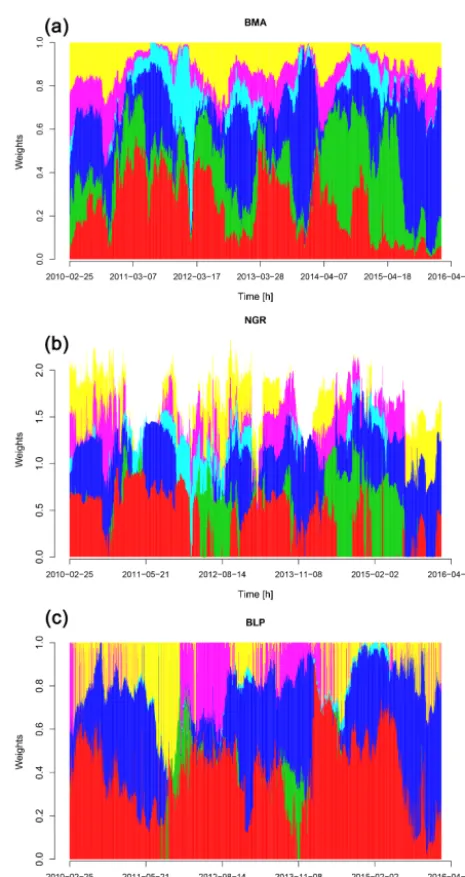
Figure 2. Hourly weights of the BMA (a), NGR (b), and

BLP(c)methods estimated for a lead time of 48 h. The six forecasts

are the QRNN method for the COSMO-LEPS with quantile averag-ing (QRNN-CL-q.) – M1, probability averagaverag-ing (QRNN-CL-p.) – M2, the waveVARX(-CL) method – M3, the raw COSMO-LEPS (CL) forecast – M4, the two post-processed C7 forecasts based on QRNN with the EMP – M5, and the LN approach – M6.

tested as well, but 7 days was chosen finally as a trade-off between computing time and efficiency. In Fig. 2 an example of the temporal evolution of the hourly weights for a lead time of 48 h for the three combination methods is shown.

fore-Raw COSMO−LEPS

0.0 0.2 0.4 0.6

Probability integral transform

0.8 1.0

01

Relativ

e

f

requency

2

3

4

5

6

BLP

Relativ

e

f

requency

0.0 0.2 0.4 0.6

Probability integral transform

0.8 1.0

012345

6

NGR

0.0 0.2 0.4

Probability integ ral transform

0.6 0.8 1.0

01

Relativ

e

f

requency

2

3

4

5

6

BMA

0.0 0.2 0.4 0.6

Probability integral transform

0.8 1.0

01

Relativ

e

f

requency

2

3

4

5

6

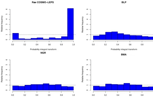
Figure 3.Probability integral transform (PIT) of the raw and three combined forecasts at a lead time of 48 h.

casts, the sequence of PIT values will follow a uniform dis-tribution U (0,1). U-shaped PIT histograms indicate under-dispersed forecasts with too little spread on average, and in-verse U-shaped histograms correspond to overdispersed fore-casts (see for example Gneiting et al., 2007; Laio and Tamea, 2007).

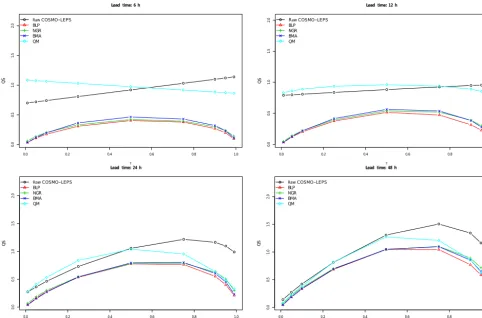
The question now is whether there are significant differ-ences between the three combination methods. Therefore the QS has been applied at first to highlight possible differences between the combination methods in more detail.

In Fig. 4 the results of the QS at four lead times for the raw COSMO-LEPS (C-L, black line) and for the three combina-tion methods BLP (red line), NGR (green line), and BMA (blue line) are shown and compared to the QS results of the raw C-L (black circles). Additionally, a simple quantile map-ping (QM) is applied (cyan diamonds) to the raw C-L fore-casts in order to evaluate the positive effect of using more complex methods. Thereby the cdf of the raw forecast is matched to the cdf of the observations. As mentioned in Zhao et al. (2017), QM is highly effective for bias correction, but ensemble spread reliability problems cannot be solved prop-erly.

In Fig. 5 the CRPS results of the six forecast models are shown in comparison to the BLP in order to demonstrate

the motivation of aggregating these systems. As can be seen clearly, the combined forecast outperforms each of the indi-vidual forecasts in view of the CRPS.

The CRPS for the raw C-L, the QM approach and the three combination methods is shown in Fig. 6.

4 Discussion

So far most of the studies comparing the results of the BMA and the NGR approach have not found any preference (see for example Williams et al., 2014). In this paper these two methods are checked against the BLP, which has not been used for hydrological purposes until now. In a first step the weights derived for each individual, raw and post-processed, forecast system are compared. The pattern of these optimized weights in Fig. 2 shows rather vague similarities between the three combination methods. The BLP and the NGR are in general more spiky, with rapid changes between consecutive hours. This could result from problems in convergence from the optimization algorithm applied for estimating the param-eters (“constrOptim” in R R Core Team, 2016).

0.0 0.2 0.4 0.6 0.8 1.0

0.0

0.5

1.0

1.5

2.0

Lead time: 6 h

τ

QS

Raw C OS MO−LE P S BLP NGR BMA QM

0.0 0.2 0.4 0.6 0.8 1.0

0.0

0.5

1.0

1.5

2.0

Lead time: 12 h

τ

QS

Raw C OS MO−LE P S BLP NGR BMA QM

0.0 0.2 0.4 0.6 0.8 1.0

0.0

0.5

1.0

1.5

2.0

Lead time: 24 h

τ

QS

Raw C OS MO−LE P S BLP NGR BMA QM

0.0 0.2 0.4 0.6 0.8 1.0

0.0

0.5

1.0

1.5

2.0

Lead time: 48 h

τ

QS

Raw C OS MO−LE P S BLP NGR BMA QM

Figure 4.Quantile score (QS) for various lead times and the three combination methods in comparison to the raw COMSO-LEPS and a

simple quantile mapping (QM) approach.

0 10 20 30 40 50 60 70

0.5

1.0

1.5

2.0

Sihl

Lead time [h]

CRPS

M1 M2 M3 M4 M5 M6 BLP

Figure 5.CRPS of the six forecast models: COSMO-LEPS with

quantile averaging (QRNN-CL-q.) – M1, probability averaging (QRNN-CL-p.) – M2, the waveVARX(-CL) method – M3, the raw COSMO-LEPS (CL) forecast – M4, the two post-processed C7 forecasts based on QRNN with the EMP – M5, and the LN ap-proach – M6. Additionally, the CRPS of the BLP combined forecast is shown.

0 10 20 30 40 50 60 70

0.5

1.0

1.5

2.0

Lead time [h]

CRPS

Raw C OS MO−LE P S BLP NGR BM A QM

Figure 6.CRPS of the raw and combined forecasts.

certain seasons and for certain flow conditions during a year. However, the limited amount of data does not allow us to draw clear conclusions.

of the raw forecasts. The same behaviour is visible for al-most all lead times; however, the raw COSMO-LEPS fore-casts get less underdispersed with increasing lead time, since the spread and the uncertainty in the ensemble increase.

The analysis of the QS (Fig. 4) shows slightly better re-sults for the BLP, followed by the NGR and BMA. The raw COSMO-LEPS (C-L) and the QM are much worse, espe-cially for smaller lead times. It is interesting to see that the QS of the raw C-L follows a straight line for smaller lead times (6 and 12 h) in the same manner as one would expect from deterministic forecasts, because of the underdispersive-ness of the C-L at the beginning of the forecast horizon. The slope of this line is an indicator of the size of the (positive) bias. The QM at a lead time of 6 h is also a straight line, how-ever, with an opposite but much smaller and negative slope (bias) in comparison to the raw C-L. With increasing lead times the QS of the raw C-L and the QM forecasts come closer to the combined forecasts for probability levels be-tween 0.1 and 0.5. This is most probably caused by the in-creased spread of the ensemble. However, for a lead time of 24 and 48 h, the raw C-L forecasts still show the worst be-haviour at higher flows, whereas the QM method performs at a lead time of 48 h almost as well as the combination meth-ods, apart from the forecasts around the median.

As already stated previously, the comparison of the CRPS of the different post-processed methods and the aggregated ones (e.g. BLP) clearly identifies the advantage of combina-tion (Fig. 5). The CRPS, i.e. the integral of the QS, for the different combination methods (Fig. 6) confirms the results of the QS. In general the results of the BLP are slightly bet-ter than the NGR and BMA results. It seems that for those periods of lead times, where the BLP is not superior (e.g. around 20 h), the optimization routines had problems on con-vergence. However, further analysis will be necessary. The comparison with the QM approach confirmed the results of Zhao et al. (2017), since the forecast quality did not show any improvements at the first lead times because of the un-derdispersiveness of the raw C-L. Thus, the more complex combination by far outperforms the QM method.

5 Conclusions

Combination is an essential tool for improving the forecast quality. The different methods are all more or less equally suited. Although the BLP showed slightly better results, the straightforward application and the low computational costs of the NGR make this method an equally good alternative, at least for this case study. The parameter estimation of the BMA and the BLP could get quite time-consuming and sometimes results in suboptimal solutions, which could de-grade the gain of applying combination methods.

Data availability. The COSMO-LEPS and C7 raw meteorological

forecasts are properties of MeteoSwiss and have been made avail-able under license agreement between WSL and MeteoSwiss. The processed streamflow simulations and forecasts as well as the mea-sured discharge data can be made available upon request. All cal-culations of the post-processing and the combination methods have been implemented in the R statistical software (R Core Team, 2016) using various packages like QRNN (Cannon, 2011) and ensem-bleBMA (Raftery et al., 2005).

Competing interests. The authors declare that they have no conflict

of interest.

Acknowledgements. The real-time operational system for the Sihl

basin is financed by the Office of Waste, Water, Energy and Air of the Canton of Zurich. This study was conducted in the framework of the Swiss Competence Center for Energy Research – Supply of Electricity (SCCER-SoE) with funding from the Commission for Technology and Innovation – CTI (grant 2013.0288). MeteoSwiss is greatly acknowledged for providing all used meteorological data. The Swiss Federal Office for Environment (FOEN) provided the observed discharge data. The authors would like to thank especially Vanessa Round for proofreading.

Edited by: Florian Pappenberger Reviewed by: two anonymous referees

References

Abrahart, R. J. and See, L.: Multi-model data fusion for river flow forecasting: an evaluation of six alternative methods based on two contrasting catchments, Hydrol. Earth Syst. Sci., 6, 655–670, https://doi.org/10.5194/hess-6-655-2002, 2002.

Addor, N., Jaun, S., Fundel, F., and Zappa, M.: An operational hydrological ensemble prediction system for the city of Zurich (Switzerland): skill, case studies and scenarios, Hydrol. Earth Syst. Sci., 15, 2327–2347, https://doi.org/10.5194/hess-15-2327-2011, 2011.

Ajami, N. K., Duan, Q., and Sorooshian, S.: An integrated hy-drologic Bayesian multimodel combination framework: Con-fronting input, parameter, and model structural uncertainty in hydrologic prediction, Water Resour. Res., 43, W01403, https://doi.org/10.1029/2005WR004745, 2007.

Baran, S.: Probabilistic wind speed forecasting

us-ing Bayesian model averaging with truncated normal

components, Comput. Stat. Data An., 75, 227–238,

https://doi.org/10.1016/j.csda.2014.02.013, 2014.

Baran, S. and Lerch, S.: Log-normal distribution based Ensem-ble Model Output Statistics models for probabilistic wind-speed forecasting, Q. J. Roy. Meteor. Soc., 141, 2289–2299, https://doi.org/10.1002/qj.2521, 2015.

Bates, J. and Granger, C.: The combination of forecasts, Operations Research Quarterly, 20, 451–468, 1969.

flood forecasting system, Water Resour. Res., 47, W07524, https://doi.org/10.1029/2010WR009137, 2011.

Bogner, K., Liechti, K., and Zappa, M.: Post-Processing of Stream Flows in Switzerland with an Emphasis on Low Flows and Floods, Water, 8, 115, https://doi.org/10.3390/w8040115, 2016. Bouallègue, Z. B., Pinson, P., and Friederichs, P.: Quantile forecast

discrimination ability and value, Q. J. Roy. Meteor. Soc., 141, 3415–3424, https://doi.org/10.1002/qj.2624, 2015.

Bowden, G. J., Maier, H. R., and Dandy, G. C.: Real-time de-ployment of artificial neural network forecasting models: Un-derstanding the range of applicability, Water Resour. Res., 48, w10549, https://doi.org/10.1029/2012WR011984, 2012.

Cannon, A. J.: Quantile regression neural networks:

Implementation in R and application to

precipita-tion downscaling, Comput. Geosci., 37, 1277–1284,

https://doi.org/10.1016/j.cageo.2010.07.005, 2011.

Chernozhukov, V., Fernández-Val, I., and Galichon, A.: Quantile and Probability Curves Without Crossing, Econometrica, 78, 1093–1125, https://doi.org/10.3982/ECTA7880, 2010.

Dawid, A.: Statistical theory: The prequential approach, J. Roy. Statist. Soc. A, 147, 278–292, 1984.

Diks, C. G. H. and Vrugt, J. A.: Comparison of point forecast accuracy of model averaging methods in hydro-logic applications, Stoch. Env. Res. Risk A., 24, 809–820, https://doi.org/10.1007/s00477-010-0378-z, 2010.

Dogulu, N., López López, P., Solomatine, D. P., Weerts, A. H., and Shrestha, D. L.: Estimation of predictive hydrologic uncer-tainty using the quantile regression and UNEEC methods and their comparison on contrasting catchments, Hydrol. Earth Syst. Sci., 19, 3181–3201, https://doi.org/10.5194/hess-19-3181-2015, 2015.

Fraley, C., Raftery, A., and Gneiting, T.: Calibrating multimodel forecast ensembles with exchangeable and missing members us-ing Bayesian model averagus-ing, Mon. Weather Rev., 138, 190– 202, 2010.

Friederichs, P. and Hense, A.: Statistical Downscaling of

Extreme Precipitation Events Using Censored

Quan-tile Regression, Mon. Weather Rev., 135, 2365–2378,

https://doi.org/10.1175/MWR3403.1, 2007.

Glahn, H. and Lowry, D.: The use of model output statistics (MOS) in objective weather forecasting, J. Appl. Meteorol., 11, 1203– 1211, 1972.

Gneiting, T. and Ranjan, R.: Comparing Density Forecasts Using Threshold- and Quantile-Weighted Scoring Rules, J. Bus. Econ. Stat., 29, 411–422, 2011.

Gneiting, T. and Ranjan, R.: Combining predictive distributions, Electron. J. Statist., 7, 1747–1782, https://doi.org/10.1214/13-EJS823, 2013.

Gneiting, T., Raftery, A., Westveld III, A., and Goldman, T.: Cal-ibrated probabilistic forecasting using ensemble model output statistics and minimum CRPS estimation, Mon. Weather Rev., 133, 1098–1118, 2005.

Gneiting, T., Balabdaoui, F., and Raftery, A.: Probabilistic fore-casts, calibration and sharpness, J. Roy. Stat. Soc. B, 69, 243– 268, 2007.

Hemri, S., Fundel, F., and Zappa, M.: Simultaneous cali-bration of ensemble river flow predictions over an entire range of lead times, Water Resour. Res., 49, 6744–6755, https://doi.org/10.1002/wrcr.20542, 2013.

Hemri, S., Scheuerer, M., Pappenberger, F., Bogner, K., and Haiden, T.: Trends in the predictive performance of raw en-semble weather forecasts, Geophys. Res. Lett., 41, 9197–9205, https://doi.org/10.1002/2014GL062472, 2014.

Koenker, R.: Quantile Regression, Econometric Society Mono-graphs, Cambridge University Press, New York, 2005.

Koenker, R. and Machado, J. A. F.: Goodness of

Fit and Related Inference Processes for Quantile

Regression, J. Am. Stat. Assoc., 94, 1296–1310,

https://doi.org/10.1080/01621459.1999.10473882, 1999. Laio, F. and Tamea, S.: Verification tools for probabilistic

fore-casts of continuous hydrological variables, Hydrol. Earth Syst. Sci., 11, 1267–1277, https://doi.org/10.5194/hess-11-1267-2007, 2007.

Lichtendahl, K. C. J., Grushka-Cockayne, Y., and Winkler, R. L.: Is It Better to Average Probabilities or Quantiles?, Manage. Sci., 59, 1594–1611, https://doi.org/10.1287/mnsc.1120.1667, 2013. Liechti, K., Oplatka, M., Eisenhut, N., and Zappa, M.: Early Flood

Warning for the City of Zurich: Evaluation of real-time Opera-tions since 2010, in: 13th Congress Interpraevent 2016, Living with natural risks, 2016.

López López, P., Verkade, J. S., Weerts, A. H., and Solomatine, D. P.: Alternative configurations of quantile regression for estimat-ing predictive uncertainty in water level forecasts for the upper Severn River: a comparison, Hydrol. Earth Syst. Sci., 18, 3411– 3428, https://doi.org/10.5194/hess-18-3411-2014, 2014. Min, C.-K. and Zellner, A.: Bayesian and non-Bayesian

meth-ods for combining models and forecasts with applications to forecasting international growth rates, J. Econ., 56, 89–118, https://doi.org/10.1016/0304-4076(93)90102-B, 1993.

Montani, A., Cesari, D., Marsigli, C., and Paccagnella, T.: Seven years of activity in the field of mesoscale ensemble forecasting by the COSMO-LEPS system: main achievements and open chal-lenges, Tellus A, 63, 605–624, 2011.

Quiñonero Candela, J., Rasmussen, C., Sinz, F., Bousquet, O., and Schölkopf, B.: Evaluating Predictive Uncertainty Chal-lenge, in: Machine Learning Challenges. Evaluating Predic-tive Uncertainty, Visual Object Classification, and Recognis-ing Tectual Entailment, edited by: Quiñonero Candela, J., Da-gan, I., Magnini, B., and d’Alché Buc, F., vol. 3944 of Lecture Notes in Computer Science, Springer, Berlin, Heidelberg, 1–27, https://doi.org/10.1007/11736790_1, 2006.

R Core Team: R: A language and environment for statistical com-puting. R Foundation for Statistical Computing, Vienna, Austria, https://www.R-project.org/ (last access: 30 September 2017), 2016.

Raftery, A., Gneiting, T., Balabdaoui, F., and Polakowski, M.: Using Bayesian Model Averaging to Calibrate

Fore-cast Ensembles, Mon. Weather Rev., 133, 1155–1174,

https://doi.org/10.1175/MWR2906.1, 2005.

Raftery, A. E., Madigan, D., and Hoeting, J. A.: Bayesian Model Averaging for Linear Regression Models, J. Am. Stat. Assoc., 92, 179–191, https://doi.org/10.1080/01621459.1997.10473615, 1997.

Ranjan, R. and Gneiting, T.: Combining

probabil-ity forecasts, J. Roy. Stat. Soc. B Met., 72, 71–91,

https://doi.org/10.1111/j.1467-9868.2009.00726.x, 2010. Ronco, P., Bullo, M., Torresan, S., Critto, A., Olschewski, R.,

as-sessment methodology for water-related natural hazards – Part 2: Application to the Zurich case study, Hydrol. Earth Syst. Sci., 19, 1561–1576, https://doi.org/10.5194/hess-19-1561-2015, 2015. Schepen, A. and Wang, Q. J.: Model averaging methods to

merge operational statistical and dynamic seasonal streamflow forecasts in Australia, Water Resour. Res., 51, 1797–1812, https://doi.org/10.1002/2014WR016163, 2015.

Shamseldin, A., O’Connor, K., and Liang, G.: Methods for com-bining the outputs of different rainfall–runoff models, J. Hydrol., 197, 203–229, 1997.

Taylor, J. W.: A quantile regression neural network approach to es-timating the conditional density of multiperiod returns, J. Fore-casting, 19, 299–311, 2000.

Thompson, P. D.: How to Improve Accuracy by

Combining Independent Forecasts, Mon. Weather

Rev., 105, 228–229,

https://doi.org/10.1175/1520-0493(1977)105<0228:HTIABC>2.0.CO;2, 1977.

Todini, E.: A model conditional processor to assess predictive uncertainty in flood forecasting, International Journal of River Basin Management, 6, 123–137, 2008.

Van der Waerden, B. L.: Order tests for two-sample problem and their power I, Indagat. Math., 14, 453–458, 1952.

Van der Waerden, B. L.: Order tests for two-sample problem and their power II, Indagat. Math., 15, 303–310, 1953a.

Van der Waerden, B. L.: Order tests for two-sample problem and their power III, Indagat. Math., 15, 311–316, 1953b.

Vrugt, J. A. and Robinson, B. A.: Treatment of uncertainty using ensemble methods: Comparison of sequential data assimilation and Bayesian model averaging, Water Resour. Res., 43, W01411, https://doi.org/10.1029/2005WR004838, 2007.

Wallis, K. F.: Combining forecasts – forty years later, Applied Fi-nancial Economics, 21, 33–41, 2011.

Wang, Q. J., Schepen, A., and Robertson, D. E.: Merging Seasonal Rainfall Forecasts from Multiple Statistical Models through Bayesian Model Averaging, J. Climate, 25, 5524–5537, https://doi.org/10.1175/JCLI-D-11-00386.1, 2012.

Weerts, A. H., Winsemius, H. C., and Verkade, J. S.: Estima-tion of predictive hydrological uncertainty using quantile re-gression: examples from the National Flood Forecasting Sys-tem (England and Wales), Hydrol. Earth Syst. Sci., 15, 255–265, https://doi.org/10.5194/hess-15-255-2011, 2011.

Wilks, D. S.: Statistical Methods in the Atmospheric Sciences: An Introduction, Academic Press, New York, 1995.

Williams, R. M., Ferro, C. A. T., and Kwasniok, F.: A comparison of ensemble post-processing methods for extreme events, Q. J. Roy. Meteor. Soc., 140, 1112–1120, https://doi.org/10.1002/qj.2198, 2014.