Improvement of hydrological model calibration by selecting multiple parameter ranges

www.hydrol-earth-syst-sci.net/21/393/2017/ doi:10.5194/hess-21-393-2017

© Author(s) 2017. CC Attribution 3.0 License.

Improvement of hydrological model calibration by selecting

multiple parameter ranges

Qiaofeng Wu1, Shuguang Liu1,2, Yi Cai1,2, Xinjian Li3, and Yangming Jiang4

1_{Department of Hydraulic Engineering, College of Civil Engineering, Tongji University, Shanghai, 200092, China} 2_{Key Laboratory of Yangtze River Water Environment, Ministry of Education, Shanghai, 200092, China}

3_{Guangxi Zhuang Autonomous Region Center Station of Irrigation Experiment, Guilin, 541105, China}

4_{Hydrology & Water Resources Bureau of Guilin, Guangxi Zhuang Autonomous Region, Guilin, 541001, China} Correspondence to:Yi Cai ([email protected])

Received: 31 May 2016 – Published in Hydrol. Earth Syst. Sci. Discuss.: 20 June 2016 Revised: 10 December 2016 – Accepted: 14 December 2016 – Published: 24 January 2017

Abstract.The parameters of hydrological models are usually calibrated to achieve good performance, owing to the highly non-linear problem of hydrology process modelling. How-ever, parameter calibration efficiency has a direct relation with parameter range. Furthermore, parameter range selec-tion is affected by probability distribuselec-tion of parameter val-ues, parameter sensitivity, and correlation. A newly proposed method is employed to determine the optimal combination of multi-parameter ranges for improving the calibration of hy-drological models. At first, the probability distribution was specified for each parameter of the model based on genetic algorithm (GA) calibration. Then, several ranges were se-lected for each parameter according to the corresponding probability distribution, and subsequently the optimal range was determined by comparing the model results calibrated with the different selected ranges. Next, parameter correla-tion and sensibility were evaluated by quantifying two in-dexes,RCY, XandSE, which can be used to coordinate with

the negatively correlated parameters to specify the optimal combination of ranges of all parameters for calibrating mod-els. It is shown from the investigation that the probability dis-tribution of calibrated values of any particular parameter in a Xinanjiang model approaches a normal or exponential distri-bution. The multi-parameter optimal range selection method is superior to the single-parameter one for calibrating hydro-logical models with multiple parameters. The combination of optimal ranges of all parameters is not the optimum inas-much as some parameters have negative effects on other pa-rameters. The application of the proposed methodology gives rise to an increase of 0.01 in minimum Nash–Sutcliffe

effi-ciency (ENS) compared with that of the pure GA method.

The rising of minimumENSwith little change of the

maxi-mum may shrink the range of the possible solutions, which can effectively reduce uncertainty of the model performance.

1 Introduction

models do, especially for catchments lacking sufficient data (Bao et al., 2010; Cullmann et al., 2011). Thus, many con-ceptual models such as HBV model, TOPMODEL, Tank model and Xinanjiang model are of strong vitality (Abebe et al., 2010; Vincendon et al., 2010; Hao et al., 2015; Xie et al., 2015). Additionally, the performance of physically based distributed models can be improved after calibration of some parameters (Chen et al., 2016). Therefore, all of the hydro-logical models should be calibrated before engineering ap-plications.

There are two kinds of calibration methods for hydro-logical models, the trial–error method and auto-calibration method. The trial–error method depends on plenty of trials for reducing the error of the objective. However, it is diffi-cult to obtain an exact optimal solution due to limited enu-meration (Boyle et al., 2000). The auto-calibration method is based on stochastic or mathematical calculations and thus more widely applied in the non-linear parameter optimiza-tion. Compared with the trial–error method, it is more ef-ficient and effective, avoiding the interference of anthro-pogenic factors (Madsen, 2000; Getirana, 2010). The ini-tial automatic optimization methods, such as the Rosenbrock method (Rosenbrock, 1960) and the simplex method (Nelder and Mead, 1965), are classical and useful methods, but at the same time have a negative side of being bounded by initial value ranges of parameters. Therefore, it can only be regarded as local optimization algorithms (Gupta and Sorooshian, 1985). Different from classical methods above, the genetic algorithm (GA), which is designed with random search strategy, can avoid the problem of local search and thus is a global optimization algorithm in its essence (Wang, 1991, 1997; Sedki et al., 2009; Chandwani et al., 2015). Af-ter that, many global optimization algorithms have been pro-posed inheriting the random search strategy. The shuffled complex evolution (SCE-UA) method combines many ad-vantages of the GA and simplex methods, having a power-ful capability of calibrating the rainfall–runoff model (Duan et al., 1994; Zhang and Shi, 2011). The particle swarm op-timization (PSO) based on random solution can directly ob-tain the identification parameters through the iterative search for an optimal solution (Kennedy, 1997; Zambrano-Bigiarini and Rojas, 2013). Although the auto-calibration method has been intensively employed to calibrate parameters in the field of hydrology, the most advanced algorithm inevitably falls into local solution because of the strong non-linear problem of a hydrological model and parameter correlation (Chu et al., 2010; Jiang et al., 2010, 2015).

In general, parameter variables follow some specific prob-ability distributions within the given range after multiple in-dependent calibrations (Viola et al., 2009; Jin et al., 2010; Li et al., 2010). Graziani et al. (2008) stated that the shape of a parameter probability distribution can be significantly af-fected by a parameter range. Touhami et al. (2013) studied the effect of different probability distributions (e.g. normal distribution and uniform distribution) of parameter values on

parameter sensitivity, and found that the probability distri-bution can provide a clue for realizing parameter sensitiv-ity. Although normal and uniform distributions are greatly studied in practice, other types of probability distributions were seldom investigated in previous research (Kucherenko et al., 2012; Esmaeili et al., 2014).

Most hydrological models contain many parameters of dif-ferent sensitive characteristics and correlation patterns. Some researchers believe that the sensitive parameter should be cal-ibrated, while the insensitive parameter can be set as a fixed value by experience (Beck, 1987; Cheng et al., 2006). In-appropriate parameter ranges or fixed values may result in the instability of calibrated results. Furthermore, the range setting of one parameter may influence the calibration of other related parameters (Song et al., 2015). The model pa-rameter sensitivity analysis has been a growing concern in recent years. Parameter sensitivity varies with catchment characteristics, objective functions, and parameter ranges (van Griensven et al., 2006). Wang et al. (2013) noted the different parameter ranges could lead to changes in parame-ter sensitivity. Shin et al. (2013) reported that reducing or ex-tending ranges might render insensitive parameters into sen-sitive ones or vice versa. Thus, parameter ranges and correla-tion should be taken into consideracorrela-tion when the calibracorrela-tion of multi-parameter models is performed.

Parameter ranges are generally given roughly due to lack of knowledge concerning physical settings of a local catch-ment (Song et al., 2013; Hao et al., 2015). The more devia-tion between an optimal range and a given range, the more uncertainty of the calibration result. The selection of appro-priate parameter ranges is critical for calibrating the model efficiently. However, there have not been many documented studies on how to select the appropriate parameter range for improving the calibration of hydrological models. Further-more, the calibration of multiple parameters is more complex due to parameter sensitivity and correlation. Hence, it is nec-essary to find a way to coordinate the range settings of all parameters.

2 Study area and data collection

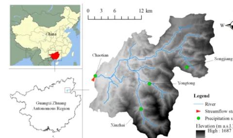
The Chaotianhe River catchment is located in the northeast of the Guangxi Zhuang Autonomous Region in southwest China (Fig. 1). The Chaotianhe River is the major tributary of the Lijiang River of a well-known karst landscape. The total catchment area is 476.24 km2. The annual precipitation is ap-proximately 1704 mm and 78 % precipitation concentrates in flood seasons (March–August). The thickness of soil varies spatially in most karst areas. Limestone is exposed to air in some peak-cluster regions. Clay soil with thickness ranging from 2 to 10 m is distributed in the depressions and valleys. In clastic rock mountain areas, the thickness of the soil is usu-ally less than 0.5 m. Thus, the soil moisture storage capacity varies significantly with space. Moreover, the underground rivers are very well developed in the karst area, which makes the flood gather rapidly and recess slowly due to higher un-derground flow rate.

The data concerning daily precipitation, evaporation and streamflow were collected from national gauging stations for the 5-year period of 1996–2000. Four precipitation stations, one streamflow gauging station, and one evaporation station are selected for the investigation. Areal precipitation was cal-culated using data from the four precipitation stations by using a Thiessen polygon method under GIS environment (Cai et al., 2014). The streamflow gauging station is at the catchment outlet. Some hydro-meteorological statistical data of the studied catchment are summarized in Table 1. From 1996 to 2000, the maximum of daily streamflow was about 719 m3s−1, the minimum 0.53 m3s−1, and the average was 13.31 m3s−1at the outlet. The maximum areal daily precipi-tation varies with years in the studied catchment and reached the value of 235 mm d−1in 1996.

3 Methodology

3.1 Hydrological model selection

The method of PRS is designed for most of hydrological models. At present, there have been many hydrological mod-els for hydrological process simulation. Considering the cli-mate characteristics of the study area, the Xinanjiang model, which is suitable for humid regions, was chosen to serve as a hydrological model for the investigation. The Xinanjiang model mainly includes three evapotranspiration layers and three runoff components (i.e. surface-, subsurface runoff and groundwater) (Zhao, 1992). The surface runoff is routed by the Unit Hydrograph (UH) which is derived from the ob-served streamflow, and other runoff components are simpli-fied as linear reservoirs (Ju et al., 2009). With regard to the Xinanjiang model, there are 10 parameters that should be cal-ibrated. The definitions of the parameters are given in Ta-ble 2 (Lin et al., 2014; Hao et al., 2015). The proposed PRS

Table 1.Metro-hydrological statistical data of the study area.

Year QMax QMin QAvg PMax

(m3s−1) (mm d−1) 1996 719 0.76 14.38 235 1997 308 0.76 14.32 155 1998 369 0.66 13.67 157 1999 282 0.53 12.81 144 2000 339 1.14 11.37 107

QMax,QMin, andQAvgmean the maximum, minimum, and average value of daily streamflow, respectively, andPMax means the maximum value of daily precipitation.

Figure 1.Location of the study area.

method is introduced as follows, when a Xinanjiang model is taken as an example.

3.2 Probability distribution analysis of calibrated parameter value

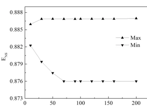
3.2.1 Sample collection of calibrated parameter value In theory, the parameter values calibrated by using a stochastic-based auto-calibration method are not the same as each other but follow a specific probability distribution un-der a reasonable convergence condition (Jiang et al., 2015). The stochastic-based auto-calibration is used to calibrate the model, and samples of calibrated parameter values are ob-tained in order to analyse the probability distribution of pa-rameter values. The sample size of 100 is adequate for es-timating the probability distribution of calibrated parameter values in the investigation, which is deduced from the results of trial tests as shown in Fig. 2. It can be seen that both max-imum and minmax-imumENSkeep stable when sample size is

greater than 100.

Table 2.Parameters of Xinanjiang model.

Parameter Definition Units

CI Recession constants of the lower interflow storage dimensionless Kc Ratio of potential evapotranspiration to pan evaporation dimensionless KI Outflow coefficients of the free water storage to interflow dimensionless SM Areal mean free water capacity of the surface soil layer, which represents

the maximum possible deficit of free water storage mm

B Exponential parameter with a single parabolic curve, which represents

the non-uniformity of the spatial dimensionless WM Averaged soil moisture storage capacity of the whole layer mm

C Coefficient of the deep layer, which depends on the proportion

of the basin area covered by vegetation with deep roots dimensionless EX Exponent of the free water capacity curve influencing the development of the saturated area dimensionless CG Recession constants of the groundwater storage relationships dimensionless KG∗ Outflow coefficients of the free water storage to groundwater relationships dimensionless Im Percentage of impervious and saturated areas in the catchment dimensionless

∗_{The value of KG is calculated by the function 0.7-KI.}

Figure 2.Variation curves of maximum and minimumENSwith

sample sizes.

model than other algorithms do (Cooper et al., 1997; Jha et al., 2006; Zhang et al., 2009). The Nash–Sutcliffe efficiency (ENS) was chosen as an objective function (Eq. 1) for GA,

which represents the agreement between observed and simu-lated data.

ENS=1−

Pn i=1

Qobs,i−Qsim,i

2

Pn i=1

Qobs,i−Qmean

2, (1)

whereENSis Nash–Sutcliffe efficiency,iis the serial number

of the step,nis the total number of the observed streamflow data,Qobs,iis the observed streamflow at stepi,Qsim,iis the simulated streamflow at stepi, andQmeanis the mean value

of observed streamflow.

3.2.2 Determination of probability distribution types

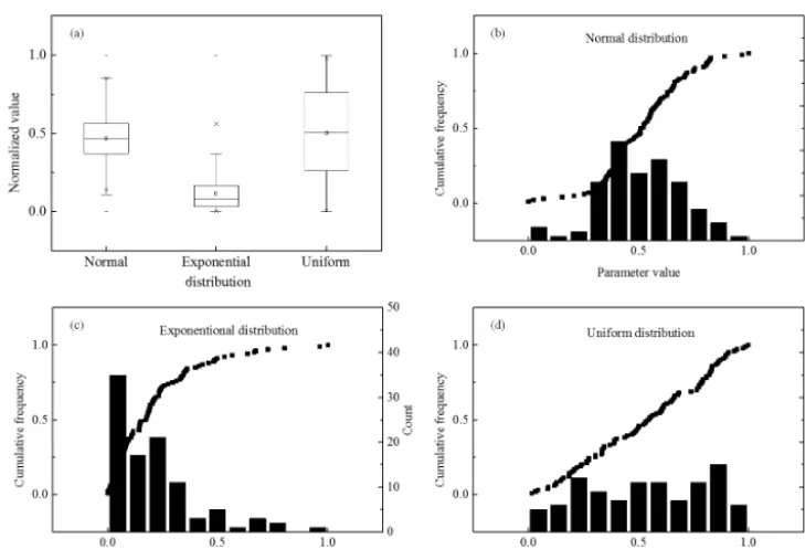
devia-Figure 3.Different probability distribution types of calibrated parameter values.(a)Box-plot charts of normal, exponential, and uniform distribution; cumulative frequency curve and histogram for normal(b), exponential(c), and uniform(d)distributions.

tion between the two values,1Max, is expressed in Eq. (2). 1Max=

F_i∗−Fi

(2)

According to the acceptable level of significance α (α= 0.2α) and the total number of values in a data setn,1table

can be obtained from the K–S table. If 1Max< 1table, the

reference probability distribution is identified to fit to the data set.

3.3 Parameter range selections

3.3.1 Single parameter range selection (S-PRS)

In order to improveENS, the initial range of a parameter

re-quires adjusting properly. Given the three probability distri-bution types mentioned above, the different ways to specify the optimal range for a single parameter are presented in the investigation. For the parameter of a uniform distribution, it is better to keep the initial range due to the weak influence of ranges on calibration results. For the parameter of a normal distribution, the cumulative frequency curve is employed to seek some reduced ranges with a given cumulative frequency (e.g. 50 %), and the minimum and maximum ranges (namely MINR and MAXR) are obtained as depicted in Fig. 4. The MINR and MAXR represent the ranges of maximum and minimum probability density of parameter values under a given cumulative frequency. As for the parameter of an ex-ponential distribution, the initial range can be extended ap-propriately towards one side of high probability density, if

the parameter has reasonable meaning in the extended range. Then, the optimal range of the parameter can be specified by comparing differentENS calculated separately by using

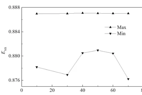
the initial range, the MINR or MAXR of the initial range, or the MINR or MAXR of the extended range. If the initial range cannot be extended, the MINR and MAXR are sought out according to the cumulative frequency curve. Figure 5 gives the variation curves of maximum and minimumENS

of a single parameter with cumulative frequency values. It is found that the maximumENSremains constant despite a

cu-mulative frequency value varying, while the minimumENS

approaches the peak value of 0.881 when the cumulative fre-quency value is equal to 50 %. Considering that higher mini-mumENScontributes to more efficient calibration, the fixed

cumulative frequency value of 50 % was selected to deter-mine the ranges of maximum and minimum probability den-sity (i.e. MINR and MAXR) for each parameter. In short, the optimal range of a single parameter can be determined by properly extending or reducing the initial range to make cali-brated parameter values distributed quite closely to a uniform distribution.

Figure 4.Selection of minimum and maximum range (MINR and MAXR) with a cumulative frequency of 50 %.

Figure 5.Variation curves of maximum and minimumENSof a

single parameter with cumulative frequency values.

WM results in a smaller B (Zhao, 1992). As a result, the range change of parameter WM may affect the range setting and calibration of parameterB. If the ranges of the related parameters required adjusting, the correlations among pa-rameters, therefore, should be taken into account. If the range change of one parameter has positive influence on calibration of other parameters, using the optimal range of the parameter instead of the initial one can contribute to better calibration results. On the contrary, the negative impact may result in a worse model calibration, even though the optimal ranges of the parameters are used. Thus, some coordination measures should be taken to deal with such a contradiction. The index RC(Eq. 3) was quantified to analyse the influence degree of

one-parameter range change on the calibration of other pa-rameters. When RCY, X is closer to 1, the range change of parameterXhas a greater positive influence on the calibra-tion of parameterY. IfRCY, Xis minus, it exerts a negative

influence. RCY, X=1−

LY, X−LY, Y LY,Initial−LY,Y

, (3)

whereRCY, Xis the influence degree of the range change of parameterXon the calibration of parameterY,LY, Xis the range of parameterY calibrated with the optimal range of parameterXand initial ranges of other parameters,LY, Y is the range of parameterY calibrated with the optimal range of parameterY and initial ranges of other parameters, and LY,Initial is the range of parameter Y calibrated with initial

ranges of all parameters. The calibrated range of any param-eter is calculated, excepting extreme outliers.

If there is a negative influence between two parameters, the optimal range of the parameter of higher sensitivity is used and the initial range of the other parameter is kept for calibra-tion generally to mitigate the negative impact. It is due to the fact that sensitive parameters play more important roles than insensitive parameters do in a multi-parameter calibration. In order to assess the sensitivity of parameter range change to ENS, indexSE as expressed in Eq. (4) is computed by

per-forming an S-PRS method on each parameter. The larger the value ofRC, the more concentrated the distribution ofENS,

which means more efficient parameter calibration. Thus, the parameter of higherSEis given priority to the optimal range

when theRCof two parameters is minus.

SE=1−

E0NS Max−E0NS Min ENS Max−ENS Min

, (4)

whereSE is sensitivity of parameter range change toENS, ENS Max andENS Minare maximum and minimumENS

cali-brated with an initial range, andE0NS Max andE0NS Min are

maximum and minimum ENS calibrated with an optimal

range. The statistical analysis ofENSexcludes extreme

out-liers.

Given the fact that there are more than two parameters in most hydrological models, the accumulative influence and the coordination of range selection were investigated in the study. The mean value ofRC(RC mean) is the index to judge

the accumulative influence of one-parameter range change on the calibration of other parameters. Thus, for parameters of a negativeRC mean, the initial ranges instead of the optimal

Figure 6.The flow chart of multiple parameter range selections.

seek the optimal range for calibration when the extension of the parameter range is limited; for a uniform distribution, the initial range is kept. In stage 3, the single-parameter range selection (S-PRS) is performed on each parameter. Based on

the indexesSEandRCestimated, the optimal combination of

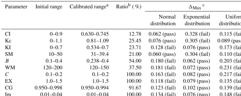
Table 3.Range changes and K–S tests (α=0.2) of parameters in the initial schema.

Parameter Initial range Calibrated rangea Ratiob( %) 1Maxc

Normal Exponential Uniform distribution distribution distribution CI 0–0.9 0.630–0.745 12.78 0.062 (pass) 0.328 (fail) 0.115 (fail) Kc 0–1.1 0.81–1.09 25.45 0.076 (pass) 0.305 (fail) 0.089 (pass) KI 0–0.7 0.534–0.7 23.71 0.128 (fail) 0.076 (pass) 0.173 (fail) SM 10–50 31–39.4 21.00 0.060 (pass) 0.304 (fail) 0.110 (fail)

B 0.1–0.4 0.238–0.4 54.00 0.180 (fail) 0.062 (pass) 0.203 (fail) WM 120–200 120–150 37.50 0.181 (fail) 0.072 (pass) 0.231 (fail)

C 0.1–0.2 0.1–0.2 100.00 0.163 (fail) 0.082 (pass) 0.217 (fail) EX 1.0–1.5 1.0–1.5 100.00 0.118 (fail) 0.079 (pass) 0.135 (fail) CG 0.950–0.998 0.950–0.994 91.67 0.123 (fail) 0.102 (pass) 0.139 (fail) Im 0.01–0.04 0.01–0.04 100.00 0.134 (fail) 0.076 (pass) 0.148 (fail)

a_{The calibrated parameter range except the extreme outlier.}

b_{The ratio is calculated by dividing the length of the range derived from 100 GA calibration runs by the initial range length.} c_The1

Maxis calculated by using the normalized parameter values.

4 Results and discussion

4.1 Probability distribution characteristics of calibrated parameter values of the Xinanjiang model

A series of calibrated parameters values were obtained through 100 independent calibration runs by using a GA method. Trial tests were employed to determine the optimal GA control parameters: crossover probability of 0.5, muta-tion probability of 0.7 for the individual, mutamuta-tion probabil-ity of 0.5 for each gene, population size of 21, maximum generation number of 500, and maximum iteration number of 50. These parameters were kept constant for GA calibra-tions in the investigation. The initial and calibrated ranges of parameters are presented in Table 3. The ratio of the cal-ibrated range length to the initial one in Table 3 is less than 60 % for most parameters (i.e. parameter CI, Kc, KI, SM,B, and WM), which implies that reducing the ranges can help calibrate most parameters efficiently. For any particular pa-rameter, calibrated values were normalized by dividing a de-viation between a calibrated value and the lower limit of the initial range by the length of the initial range. Based on 100 calibrated values after normalization, a box plot for a param-eter is depicted. It is obvious from Fig. 7 that the box and whiskers are approximately symmetrical and the length of whiskers is longer than that of half the box along the direc-tion of the y axis for parameters CI, SM, and Kc. But for other parameters, it is shown from the box-plot charts that the mean value deviates from the median one, which means an asymmetric chart. According to the characteristics of the box plots, the probability distributions of the calibrated val-ues are normal for parameters CI, SM, and Kc, while those are exponential for other parameters. Furthermore, K–S tests

Figure 7.The box-plot chart of normalized calibrated values for parameters of Xinanjiang model.

were employed to determine the probability distributions of parameters and the corresponding results are listed in Ta-ble 3. It is shown that only a normal distribution is accepted for parameters CI and SM. Despite the fact that both normal and uniform distributions are accepted for parameter KC, the probability distribution of parameter KC is regarded as a nor-mal distribution. It is because the1Maxwill become smaller

and Im. It indicates that reducing the initial ranges can im-prove the calibration for parameters whose values observe normal distributions.

4.2 Effect of range adjustment pattern on calibration results

Since the probability distribution of a single parameter has a direct relation with the PRS, the range adjustment pattern of a single parameter was discussed on the basis of the parameter probability distribution in the investigation.

For a normal distribution, the range was reduced to find the optimal range. Figure 8 shows the calibration results of pa-rameter CI when the different ranges are selected. The MINR (0.679–0.713) and the MAXR (0.623–0.694) were picked out based on the cumulative frequency curve derived from calibrations with the initial range (0–0.900). From the cumu-lative curves and the histograms in Fig. 8a, b, and c, it is found that the probability distribution of parameter CI values is converted from a normal distribution to a uniform distribu-tion when the initial range is reduced to the MINR, whereas the probability distribution approximates an exponential one when the MAXR is used. Figure 8d reveals the contribution of the PRS toENS. It is found that the minimumENS,

except-ing extreme outliers, rises from 0.881 to 0.884 and theENS

concentrates at a higher value range, when the MINR is used instead of the initial range. Using the reduced range of high probability density is, therefore, helpful to make calibration more stable and more efficient.

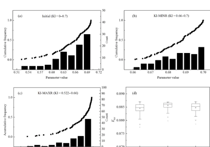
To an exponential distribution, both reduced ranges and extended ranges of reasonable meaning were used to select the optimal range for parameter calibration. Figure 9 shows the calibration results under three different input ranges of parameter KI. Since the initial range of parameter KI cannot be extended, the two reduced ranges (i.e. the MINR, 0.660– 0.700, and the MAXR, 0.522–0.660) were picked out accord-ing to the cumulative frequency curve. From the cumulative curves and the histograms in Fig. 9a, b, and c, it is found that the probability distribution of parameter KI values is similar to a uniform distribution in the case of the MINR, whereas that is still exponential in the case of the MAXR. The con-tributions of the three parameter ranges toENSare shown in

Fig. 9d. Thus, the MINR is best for calibration of parame-ter KI when compared with the MAXR or the initial range, which is similar to the calibration result of parameter CI. In general, the MINR is better than the MAXR for parameter calibration, because the parameter values that may achieve a higher ENS can be easily picked out from the MINR of

higher probability density.

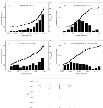
Figure 10 shows the calibration results of parameter B whose initial range can be extended. ParameterBgenerally ranges from 0.1 to 0.4 for most areas, but it is quite different for karst areas where the soil moisture storage varies remark-ably with space. As a result, the value of parameter B can be greater than 0.4. From Fig. 10a and b, it is shown that

the probability distribution of parameterBis converted from an exponential distribution to a normal distribution when the initial range is extended to new one (B=0.1–0.6). After the MINR selection was performed on the initial range and the extended range, the two ranges, i.e. the MINR (B=0.36– 0.40) and the extension-MINR (B=0.379–0.488), were ob-tained and then used to calibrate parameterB. From Fig. 10c and d, it is found that the probability distribution of param-eterB approximates a uniform distribution when the MINR or the extension-MINR is used. The box plots ofENSfor

dif-ferent ranges are shown in Fig. 10e. It is shown that there is little improvement in maximumENSwhen MINR is used for

calibration instead of the initial range. There is an increase of 0.0003 in maximumENSif the initial range is replaced with

the extension range or the extension-MINR. As for minimum ENS(except outliers), an increase of 0.001 in the case of the

MINR, a decrease of 0.003 in the case of the extension range, and an increase of 0.003 in the case of the extension-MINR are found when they replace the initial range. It suggests that an appropriate range extension followed by a MINR selec-tion is helpful to improve calibraselec-tion for the parameter whose probability distribution is exponential and initial range can be extended.

4.3 Effect of multiple parameter range combination on calibration results

The S-PRS method was employed to determine the optimal range for each parameter. According to the optimal ranges and the corresponding initial ranges, indexedRCandSEwere

quantified to understand parameter correlation and sensitiv-ity. It is obvious from Table 4 thatRCvalues in the columns

of parameters CI and WM are positive, but mostRCvalues

in the column of parameter Im are negative. The negative RC related to two parameters means that using the optimal

range of one parameter is adverse to calibrating the other. BothRC EX,Im andRC Im,EX are negative in spite of small

values, indicating that using the optimal ranges of parame-ters EX and Im simultaneously is not conducive to calibrat-ing these two parameters. The mean ofRC(RC mean) varies

with parameters. Parameter CI has the maximumRC meanof

0.465 and parameter Im the minimum RC mean of −0.026.

Furthermore, all parameters have positiveRC meanvalues

ex-cept for parameter Im, owing to the accumulative negative correlation between parameter Im and the others.

To coordinate with negatively related parameters, the in-dexSEwas used to pick out parameters of higher sensitivity

toENS. From Table 4, it is found that parameter CI has the

maximumSEof 54.7 % and parameter Im the minimumSE

of 0.3 %. MostSE values are more than 20 % except those

of parameters C, EX, and Im. It suggests that parameters C, EX, and Im are of low sensitivity to ENS and the

oth-ers highly sensitive toENS. Parameter CI is the most

well-Figure 8.Results of range selection of parameter CI. Probability distribution of parameter values for schema initial range(a), CI-MINR(b)

and CI-MAXR(c);(d)box-plot chart ofENSfor three schemas.

Figure 9.Results of range selection of parameter KI. Probability distribution of parameter values for schema initial range(a), KI-MINR(b), and KI-MAXR(c);(d)box-plot chart ofENSfor three schemas.

developed karst areas, the thin layer of soil and strong per-meability of limestone make rainfall easy to penetrate into the ground. Moreover, the existence of karst caves and sub-surface streams contribute to great interflow storage which accounts for a large proportion of streamflow. As a result,

Figure 10.Results of range selection of parameterB. Probability distribution for schema initial range(a),B-Extension(b),B-MINR(c), andB-Extension-MINR(d);(e)box-plot chart ofENSfor four schemas.

Table 4.The indexedRCandSEof parameters when the optimal range of each parameter is used for calibration.

Parameter∗ _{CI Kc KI SM B WM C EX CG Im}

Optimal range of 0.679–0.713 0.95–1.05 0.66–0.7 35–39 0.379–0.488 105–110 0.175–0.2 1–1.118 0.95–0.966 0.01–0.0245 a single parameter

R_C

CI 1.000 0.334 0.371 0.462 0.322 0.113 0.105 0.115 −0.128 0.272

Kc 0.689 1.000 0.467 0.429 0.504 0.503 0.389 0.102 0.284 0.150

KI 0.778 0.315 1.000 0.445 0.574 0.268 0.456 0.328 0.060 0.258

SM 0.508 −0.199 0.422 1.000 −0.089 0.009 −0.063 0.383 0.218 −0.032

B 0.914 0.560 0.698 −0.017 1.000 0.972 −0.175 0.007 −0.319 −0.722

WM 0.575 0.311 0.439 0.553 0.325 1.000 0.229 0.360 −0.069 −0.235

C 0.208 0.273 0.083 0.151 0.277 0.335 1.000 0.077 0.200 0.210

EX 0.054 0.047 −0.011 0.018 0.371 0.045 0.009 1.000 −0.021 −0.025

CG 0.221 0.246 −0.135 0.022 0.010 0.198 −0.034 −0.009 1.000 −0.112

Im 0.238 0.073 −0.025 0.045 0.031 0.030 −0.026 −0.020 0.001 1.000

Mean ofRC 0.465 0.218 0.257 0.234 0.258 0.275 0.099 0.149 0.025 −0.026

SE(%) 54.7 47.9 36.6 41.7 48.1 39.9 10.8 14.7 21.9 0.3

∗_{The parameter represents parameter}

Table 5.Parameter range setting for different cases.

Case Range setting of parameter

CI Kc KI SM B WM C EX CG Im

1 I I I I I I I I I I

2 I I I I I I I I I O

3 I I I I I I I O I I

4 I I I I I I I O I O

5 O O O O O O O O I I

6 O O O O O O O O O I

7 O O O O O O O O O O

The symbol “I” represents the initial range of the parameter in Table 3, and “O” the optimal range of the parameter in Table 4.

ranges of parameters of higher sensitivity should be used to improve calibration.

In order to determine the optimal range combination of multiple parameters, seven cases were investigated with dif-ferent range combinations of parameters (Table 5). Case 1 was defined as the initial case using all initial ranges. Cases 2–4 were defined as the single parameter range se-lection (S-PRS) cases. Cases 5–7 were set as the multiple parameter range selection (M-PRS) cases. The box plots of ENS for different cases are given in Fig. 11. There is a

small decrease inENSwhen Case 4 is separately compared

with Cases 1–3. It can be explained that both RC EX,Imand RC Im,EX are negative and the combination of the optimal

ranges corresponding to the two parameters leads to a worse calibration result. As the SE value of parameter Im is less

than that of parameter EX, parameter EX is given priority to use the optimal range. It is the reason why the calibra-tion result of Case 3 is better than that of Case 2. As for the cases with the multi-parameter range selection (i.e. Cases 5– 7), theENS values are more robust than those of Cases 1–

4. There is an increase of approximately 0.001 in maximum ENS and an increase of approximately 0.01 in minimum ENSwhen the multi-parameter range selection is performed.

There are some differences inENSwith the comparison

be-tween Cases 5–7 in a magnified box-plot chart. Case 6 has the most concentrated values of ENS and the largest mean

value ofENSamong the three cases. It means that the

com-bination of optimal ranges of all parameters (see Case 7) is not the optimum to calibrate a multi-parameter model inas-much as some parameters like Im have negative correlation on other parameters. Hence, the initial ranges of parameters having negative mean values ofRCand low values ofSEare

supposed to be used to calibrate parameters instead of the corresponding optimal ranges.

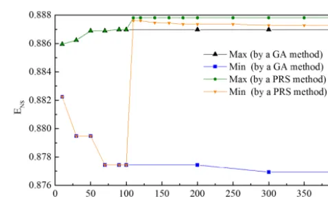
Through a calibration run, a set of calibrated values of all parameters and the correspondingENSare obtained.

Fig-ure 12 shows the variation curves of maximum and minimum values of ENS with number of runs by using a GA method

and a proposed PRS method. It is indicated from Fig. 12 that no matter if it is maximum or minimumENS, the PRS-based

Figure 11.The box-plot chart ofENSfor different cases.

Figure 12.The variation curves of maximum and minimumENS

with number of runs by using a GA method and a proposed PRS method.

value is essentially the same as the GA-based one when the number of runs does not exceed 100. It is because the PRS method initially needs 100 runs of GA calibration to obtain parameter value samples for selecting the optimal ranges. If a proposed method is used for calibration instead of a GA method, there is an increase of approximately 0.001 in max-imumENS and an increase of approximately 0.01 in

min-imum ENS when the number of runs is greater than 100.

Thus, for any particular run number, the value ofENS

cal-culated by using a PRS method is not less than that by using a GA method. Additionally, it is found from the investigation that there is no significant difference in computational time between the two methodologies. The application of a pro-posed method, therefore, contributes to a relatively efficient calibration.

5 Conclusions

pa-rameter sensitivity, and correlation between papa-rameters. The newly proposed method was applied for the calibration of a Xinanjiang model for karst areas, and some findings are pre-sented as follows.

In the Xinanjiang model, parameters CI, Kc, SM, and B approximately obey normal probability distributions and pa-rameters WM, C, EX, KI, CG, and Im obey exponential probability distributions, both after 100 independent calibra-tion runs. For the parameters of a normal distribucalibra-tion, the MINR defined by using a cumulative frequency curve of cal-ibrated values is preferred to be selected as the optimal pa-rameter range for calibration. For the papa-rameters of an ex-ponential distribution, the extension-MINR is recommended to be used for calibration if the initial range can be extended towards the high-probability side; otherwise the MINR is se-lected as the optimal range for calibration.

The proposed PRS method improves the minimum and mean values of ENS. The application of the proposed

methodology results in an increase of 0.01 in minimumENS

compared with that of the pure GA method. The rising of minimumENSwith little change of the maximum may shrink

the range of the possible solutions. As a result, the un-certainty of the model performance can be effectively con-trolled.

The M-PRS method is superior to the S-PRS one for cali-brating hydrologic models with multiple parameters. TheRC

and SE are two important indexes that can help to analyse

the sensitivity and correlation between parameters and con-sequently to coordinate with the negatively related param-eters. The initial ranges of parameters of relatively low SE

and negativeRC mean and the optimal ranges of parameters

of positiveRC mean should be preferred to be chosen for the

multi-parameter model calibration.

6 Data availability

Please contact the corresponding author to access the data in this study.

Competing interests. The authors declare that they have no conflict of interest.

Acknowledgements. The investigation is supported by the Non-profit Industry Financial Program of Ministry of Water Resources of China (no. 201401057), NFSC (no. 91225301), and the Scientific Research Foundation for the Returned Overseas Chinese Scholars, State Education Ministry (no. 2013-1792).

Edited by: G. Di Baldassarre

Reviewed by: two anonymous referees

References

Abbott, M. B., Bathurst, J. C., Cunge, J. A., O’Connell, P. E., and Rasmussen, J.: An introduction to the European Hydrological System – Systeme Hydrologique Europeen, “SHE”, 1: History and philosophy of a physically-based, distributed modelling sys-tem, J. Hydrol., 87, 45–59, doi:10.1016/0022-1694(86)90114-9, 1986.

Abebe, N. A., Ogden, F. L., and Pradhan, N. R.: Sensitivity and un-certainty analysis of the conceptual HBV rainfall–runoff model: Implications for parameter estimation, J. Hydrol., 389, 301–310, doi:10.1016/j.jhydrol.2010.06.007, 2010.

Bao, H., Wang, L., Li, Z., Zhao, L., and Zhang, G.: Hydrological daily rainfall-runoff simulation with BTOPMC model and com-parison with Xin’anjiang model, Water Science and Engineering, 3, 121–131, doi:10.3882/j.issn.1674-2370.2010.02.001, 2010. Beck, M. B.: Water quality modeling: A review of the

anal-ysis of uncertainty, Water Resour. Res., 23, 1393–1442, doi:10.1029/WR023i008p01393, 1987.

Boyle, D. P., Gupta, H. V., and Sorooshian, S.: Toward improved calibration of hydrologic models: Combining the strengths of manual and automatic methods, Water Resour. Res., 36, 3663– 3674, doi:10.1029/2000WR900207, 2000.

Cai, Y., Esaki, T., Liu, S., and Mitani, Y.: Effect of Substitute Wa-ter Projects on Tempo-Spatial Distribution of GroundwaWa-ter With-drawals in Chikugo-Saga Plain, Japan, Water Resour. Manag., 28, 4645–4663, doi:10.1007/s11269-014-0764-2, 2014. Caviedes-Voullième, D., García-Navarro, P., and Murillo, J.:

Influ-ence of mesh structure on 2D full shallow water equations and SCS Curve Number simulation of rainfall/runoff events, J. Hy-drol., 448–449, 39–59, doi:10.1016/j.jhydrol.2012.04.006, 2012. Chandwani, V., Vyas, S. K., Agrawal, V., and Sharma, G.: Soft Computing Approach for Rainfall-runoff Mod-elling: A Review, Aquatic Procedia, 4, 1054–1061, doi:10.1016/j.aqpro.2015.02.133, 2015.

Chen, Y., Li, J., and Xu, H.: Improving flood forecasting capa-bility of physically based distributed hydrological models by parameter optimization, Hydrol. Earth Syst. Sci., 20, 375–392, doi:10.5194/hess-20-375-2016, 2016.

Cheng, C.-T., Zhao, M.-Y., Chau, K. W., and Wu, X.-Y.: Us-ing genetic algorithm and TOPSIS for Xinanjiang model cal-ibration with a single procedure, J. Hydrol., 316, 129–140, doi:10.1016/j.jhydrol.2005.04.022, 2006.

Chu, W., Gao, X., and Sorooshian, S.: Improving the shuffled com-plex evolution scheme for optimization of comcom-plex nonlinear hy-drological systems: Application to the calibration of the Sacra-mento soil-moisture accounting model, Water Resour. Res., 46, W09530, doi:10.1029/2010WR009224, 2010.

Cooper, V. A., Nguyen, V. T. V., and Nicell, J. A.: Evalua-tion of global optimizaEvalua-tion methods for conceptual rainfall-runoff model calibration, Water Sci. Technol., 36, 53–60, doi:10.1016/S0273-1223(97)00461-7, 1997.

Cullmann, J., Krausse, T., and Saile, P.: Parameterising hy-drological models – Comparing optimisation and ro-bust parameter estimation, J. Hydrol., 404, 323–331, doi:10.1016/j.jhydrol.2011.05.003, 2011.

Esmaeili, S., Thomson, N. R., Tolson, B. A., Zebarth, B. J., Kuchta, S. H., and Neilsen, D.: Quantitative global sensitivity analysis of the RZWQM to warrant a robust and effective calibration, J. Hy-drol., 511, 567–579, doi:10.1016/j.jhydrol.2014.01.051, 2014. Freeze, R. A. and Harlan, R. L.: Blueprint for a physically-based,

digitally-simulated hydrologic response model, J. Hydrol., 9, 237–258, doi:10.1016/0022-1694(69)90020-1, 1969.

Getirana, A. C. V.: Integrating spatial altimetry data into the auto-matic calibration of hydrological models, J. Hydrol., 387, 244– 255, doi:10.1016/j.jhydrol.2010.04.013, 2010.

Graziani, F., Tong, C., and Graziani, F.: A Practical Global Sen-sitivity Analysis Methodology for Multi-Physics Applications, in: Computational Methods in Transport: Verification and Vali-dation, edited by: Graziani, F., Lect. Notes Comp. Sci., 62, 277– 299, doi:10.1007/978-3-540-77362-7_12, 2008.

Gupta, V. K. and Sorooshian, S.: The Automatic Calibration of Conceptual Catchment Models Using Derivative-Based Op-timization Algorithms, Water Resour. Res., 21, 473—485, doi:10.1029/WR021i004p00473, 1985.

Haktanir, T.: Practical computation of gamma frequency factors. Hydrol. Sci. J., 36, 599–610, doi:10.1080/02626669109492546, 1991

Hao, F., Sun, M., Geng, X., Huang, W., and Ouyang, W.: Cou-pling the Xinanjiang model with geomorphologic instantaneous unit hydrograph for flood forecasting in northeast China, In-ternational Soil and Water Conservation Research, 3, 66–76, doi:10.1016/j.iswcr.2015.03.004, 2015.

Huang, X., Liao, W., Lei, X., Jia, Y., Wang, Y., Wang, X., Jiang, Y., and Wang, H.: Parameter optimization of dis-tributed hydrological model with a modified dynamically dimen-sioned search algorithm, Environ. Modell. Softw., 52, 98–110, doi:10.1016/j.envsoft.2013.09.028, 2014.

Jha, M. K., Kumar, A., Nanda, G., and Bhatt, G.: Evalua-tion of tradiEvalua-tional and nontradiEvalua-tional optimizaEvalua-tion techniques for determining well parameters from step-drawdown test data, J. Hydrol. Eng., 11, 617–630, doi:10.1061/(asce)1084-0699(2006)11:6(617), 2006.

Jiang, Y., Liu, C., Huang, C., and Wu, X.: Improved particle swarm algorithm for hydrological parameter optimization, Appl. Math. Comput., 217, 3207–3215, doi:10.1016/j.amc.2010.08.053, 2010.

Jiang, Y., Liu, C., Li, X., Liu, L., and Wang, H.: Rainfall-runoff modeling, parameter estimation and sensitivity analysis in a semiarid catchment, Environ. Modell. Softw., 67, 72–88, doi:10.1016/j.envsoft.2015.01.008, 2015.

Jin, X., Xu, C.-Y., Zhang, Q., and Singh, V. P.: Parameter and mod-eling uncertainty simulated by GLUE and a formal Bayesian method for a conceptual hydrological model, J. Hydrol., 383, 147–155, doi:10.1016/j.jhydrol.2009.12.028, 2010.

Ju, Q., Yu, Z., Hao, Z., Ou, G., Zhao, J., and Liu, D.: Division-based rainfall-runoff simulations with BP neural net-works and Xinanjiang model, Neurocomputing, 72, 2873–2883, doi:10.1016/j.neucom.2008.12.032, 2009.

Kennedy, J.: The particle swarm: social adaptation of knowledge, Evolutionary Computation, 1997, IEEE International Conference on, 13-16 April 1997, IEEE, doi:10.1109/ICEC.1997.592326, 1997.

Kucherenko, S., Tarantola, S., and Annoni, P.: Estimation of global sensitivity indices for models with dependent variables, Comput. Phys. Commun., 183, 937–946, doi:10.1016/j.cpc.2011.12.020, 2012.

Li, L., Xia, J., Xu, C., and Singh, V. P.: Evaluation of the subjective factors of the GLUE method and compar-ison with the formal Bayesian method in uncertainty as-sessment of hydrological models, J. Hydrol., 390, 210–221, doi:10.1016/j.jhydrol.2010.06.044, 2010.

Lin, K., Lv, F., Chen, L., Singh, V. P., Zhang, Q., and Chen, X.: Xinanjiang model combined with Curve Number to simulate the effect of land use change on environmental flow, J. Hydrol., 519, 3142–3152, doi:10.1016/j.jhydrol.2014.10.049, 2014.

Lü, H., Hou, T., Horton, R., Zhu, Y., Chen, X., Jia, Y., Wang, W., and Fu, X.: The streamflow estimation using the Xinanjiang rainfall runoff model and dual state-parameter estimation method, J. Hy-drol., 480, 102–114, doi:10.1016/j.jhydrol.2012.12.011, 2013. Madsen, H.: Automatic calibration of a conceptual rainfall–runoff

model using multiple objectives, J. Hydrol., 235, 276–288, doi:10.1016/s0022-1694(00)00279-1, 2000.

Nelder, J. A. and Mead, R.: A simplex method for function mini-mization, Comput. J., 4, 308–313, 1965.

Papathanasiou, C., Makropoulos, C., and Mimikou, M.: Hy-drological modelling for flood forecasting: Calibrating the post-fire initial conditions, J. Hydrol., 529, 1838–1850, doi:10.1016/j.jhydrol.2015.07.038, 2015.

Rosenbrock, H.: An automatic method for finding the greatest or least value of a function, Comput. J., 3, 175–184, 1960. Sedki, A., Ouazar, D., and El Mazoudi, E.: Evolving

neu-ral network using real coded genetic algorithm for daily rainfall–runoff forecasting, Expert Syst. Appl., 36, 4523–4527, doi:10.1016/j.eswa.2008.05.024, 2009.

Sherman, L. K.: Stream Flow from Rainfall by the Unit-Graph Method, Eng. News-Rec., 108, 501–505, 1932.

Shin, M.-J., Guillaume, J. H. A., Croke, B. F. W., and Jakeman, A. J.: Addressing ten questions about conceptual rainfall–runoff models with global sensitivity analyses in R, J. Hydrol., 503, 135–152, doi:10.1016/j.jhydrol.2013.08.047, 2013.

Song, X., Kong, F., Zhan, C., Han, J., and Zhang, X.: Parame-ter identification and global sensitivity analysis of Xin’anjiang model using meta-modeling approach, Water Sci. Eng., 6, 1–17, doi:10.3882/j.issn.1674-2370.2013.01.001, 2013.

Song, X., Zhang, J., Zhan, C., Xuan, Y., Ye, M., and Xu, C.: Global sensitivity analysis in hydrological modeling: Review of con-cepts, methods, theoretical framework, and applications, J. Hy-drol., 523, 739–757, doi:10.1016/j.jhydrol.2015.02.013, 2015. Touhami, H. B., Lardy, R., Barra, V., and Bellocchi, G.:

Screening parameters in the Pasture Simulation model using the Morris method, Ecol. Modell., 266, 42–57, doi:10.1016/j.ecolmodel.2013.07.005, 2013.

van Griensven, A., Meixner, T., Grunwald, S., Bishop, T., Diluzio, M., and Srinivasan, R.: A global sensitivity analysis tool for the parameters of multi-variable catchment models, J. Hydrol., 324, 10–23, doi:10.1016/j.jhydrol.2005.09.008, 2006.

Viola, F., Noto, L. V., Cannarozzo, M., and La Loggia, G.: Daily streamflow prediction with uncertainty in ephemeral catchments using the GLUE methodology, Phys. Chem. Earth, 34, 701–706, doi10.1016/j.pce.2009.06.006, 2009.

Wang, J., Li, X., Lu, L., and Fang, F.: Parameter sensitivity analysis of crop growth models based on the extended Fourier Amplitude Sensitivity Test method, Environ. Modell. Softw., 48, 171–182, doi:10.1016/j.envsoft.2013.06.007, 2013.

Wang, Q. J.: The Genetic Algorithm and Its Application to Calibrat-ing Conceptual Rainfall-Runoff Models, Water Resour. Res., 27, 2467–2471, doi:10.1029/91wr01305, 1991.

Wang, Q. J.: Using genetic algorithms to optimise model param-eters, Environ. Modell. Softw., 12, 27–34, doi:10.1016/s1364-8152(96)00030-8, 1997.

Xie, Y., Xia, L. V., Liu, R., Mao, L., and Liu, X., Research on port ecological suitability evaluation index system and evaluation model, Frontiers of Structural and Civil Engineering, 9, 65–70, doi:10.1007/s11709-014-0258-6, 2015.

Zambrano-Bigiarini, M. and Rojas, R.: A model-independent Parti-cle Swarm Optimisation software for model calibration, Environ. Modell. Softw., 43, 5–25, doi:10.1016/j.envsoft.2013.01.004, 2013.

Zanon, F., Borga, M., Zoccatelli, D., Marchi, L., Gaume, E., Bon-nifait, L., and Delrieu, G.: Hydrological analysis of a flash flood across a climatic and geologic gradient: The September 18, 2007 event in Western Slovenia, J. Hydrol., 394, 182–197, doi:10.1016/j.jhydrol.2010.08.020, 2010.

Zhang, S. and Shi, J.: A Microwave Wetland Surface Emissivity Calibration Scheme Using SCE-UA Algorithm and AMSR-E Brightness Temperature Data, Procedia Environmental Sciences, 10, 2731–2739, doi:10.1016/j.proenv.2011.09.424, 2011. Zhang, X., Srinivasan, R., Zhao, K., and Liew, M. V.: Evaluation

of global optimization algorithms for parameter calibration of a computationally intensive hydrologic model, Hydrol. Process., 23, 430–441, doi:10.1002/hyp.7152, 2009.