Comparative study of data mining algorithms for diagnostic mammograms using Principal Component Analysis and J48

COMPARATIVE STUDY OF DATAMINING ALGORITHMS

FOR DIAGNOSTIC MAMMOGRAMS USING PRINCIPAL

COMPONENT ANALYSIS AND J48

Manju B. R. and Amrutha V. S.

Department of Mathematics, Amrita Vishwa Vidyapeetham, Amritapuri Campus, Kollam, Kerala, India E-Mail: [email protected]

ABSTRACT

Death rate among women can be considerably brought down with regard to breast cancer if an early detection is viable. The prediction or detection of breast cancer in early stages is a complicated research problem. Using datamining techniques, it is not a difficult task to make it practical. The modern researches show that in most situations these techniques work better than common diagnostic methods. The basic aim of this work is to construct a data demonstrative model which can be used to: predict breast cancer survival even in the presence of missing values in the dataset that can reveal favorable information about the essential factors that determines the chances of survival, and also partition the patients with respect to their common peculiarities. Moreover, to find out a suitable filter-classifier combination. The Principal Component Analysis (PCA) and Decision Tree (J48) are chosen as filters. Further classification process is carried out on filtered dataset using the algorithms Logistic Model Tree (LMT), Random forest and Hoeffding Tree. Decision Tree (J48), were applied to choose the most efficient one. While implementing the classifiers, the dataset for which the feature selection is carried out using PCA gives better classification accuracies. The data mining tool WEKA provides a better platform for required experimental studies. A suitable filter - classifier pair is purposed for breast cancer prognosis by analyzing the results.

Keywords: breast cancer, data mining, principal component, decision Tree (J48), logistic model tree (LMT), random forest and hoeffding tree.

1. INTRODUCTION

Nowadays, Breast cancer has become a major cause of death among women. The number of reported cases is increasing per year due to the changed lifestyles, food habits and also by hereditary reasons. Generally, the uncontrolled way of cell partitioning leads to the formation of lump called tumor. Breast tumors can be either benign or malignant. In the case of benign tumor, the cells divide in a strangely manner and shaped to an irregularity. But it won’t spread over the body. At the same time Malignanttumors can spread over the body in a short period of time. The early diagnosis of tumors will really save time for the specialists and upgrade their capability. The conventional techniques include Positron emission tomography (PET), Ultrasound, Biopsy, Magnetic resonance imaging (MRI), Mammogram, etc. for diagnosis in humans [P. Hamsagayathri and P. Sampath (2017)]. But the modern studies show that the Datamining techniques with the implementation of machine learning algorithms will produce better output than conventional methods. The term ‘Data mining’ refers to a procedure which initiates with an unstructured dataset then tries to disclose information or hidden patterns for further studies. ML algorithms can be implemented for the purpose. Machine Learning is a designing of computer algorithms which empowers the computers to grasp from given observations. [Nagesh Shukla, Markus Hagenbuchner et al. (2018)]. It has two steps: Estimation of hidden dependencies of the dataset under consideration and the application of these observed dependencies to envision the new possible outcomes of the dataset [Konstantina Kourou a, Themis P. Exarchos (2015)]. The classification refers to

a particular learning method in which the samples are categorized into finite groups. ML methods give best results in lower dimensions. Moreover, by reducing the dimensionality can eliminate unnecessary attributes, noise, results in strong learning models since the dimensionality is low. Principal component analysis (PCA) is an effective method to lessen dimension of dataset. It compresses the content of a huge, complex set of correlated attributes into some uncorrelated attributes. [Francisco Castells, Pablo Laguna et al. (2007)]. This method deals t covariance matrix or correlation matrix to evaluate Principal components [Ai-ling Teh (2010)] from the input data in terms of linear combination of the attributes of dataset. The first principal component indicates maximum variance. In this work, the effect of principal components and the decision tree algorithm J48 in breast cancer detection is compared. A suitable combination of filter-classifier is proposed for breast cancer detection. The prognosis is based on the 9 attributes present in the dataset. The experimental studies are performed using WEKA, a data mining tool.

2. RELATED WORK

More over the factors that decide chances of survival and precision of prediction are examined [Nagesh Shukla a, Markus Hagenbuchner et al. (2018)]. A comparative critique [Kanghee Park a, Amna Ali et al. 2013)] reveals that Semi-supervised learning methods visualize the survival of breast malignancies better than Artificial neural network and support vector machines. An analysis [Rohit J. Katea, Ramya Nadigba et al. (2017)] to differentiate between implementation of ML models trained with the model evaluated crosswise across distinct phases shows that more precise model to predict survival of breast malignancy for a certain state is the model trained for that particular state. Presently, Principal component analysis (PCA) has significant role in ECG signal processing [Francisco Castells, Pablo Laguna et al. (2007)]. By the detailed study of some ECG applications, it can be concluded that PCA is applied to rectify issues associated to signal processing. The comparison of distinct classification algorithms employed PCA for selecting prominent features with respect to the defined ratio R. It is impossible to find out a ideal value of R gives maximum classification accuracy. [J. Novakovic, S. Rankov (2011)]. Condition monitoring of tools utilizes datamining methods to access hidden informations vibration signals produced by the device. So, the search for suitable pair of filter and classifier results in J48 while constructing the expert system. [M. Elangovan, S. Babu Devasenapati et al. (2011)]. In marketing, the analysis of huge multivariate datasets is conducted to provide valuable information to decision makers of an organization. PCA can be applied to avoid multicorrelation present dataset. So, the stepwise procedure is studied [Cristinel Constantin (2014)]. The review of few research papers describes the importance of ML calculations to improve the security of computer systems is executed in [Philip K. Chan and Richard P. Lippman (2006)]. To determine a classifier for detecting the condition of the blade, an algorithmic classification of several faults associated with wind turbine blade is performed using statistical features. The search ends in Hoeffding Tree algorithm with highest classification accuracy [Manju B.R., A. Joshuva et al. (2018)]. The automated visual monitoring of device parts using ML techniques is well compared in [S. Ravikumar, K.I. Ramachandran et al. (2011)]. The decision tree produces better outputs. To ensure the safety of passengers, the fault detection of break system can be done by ML approach utilizing vibration signals of the brakes. Further find out the best classifier for fault detection [R. Jegadeeshwaran and V. Sugumaran (2013)].

3. METHODOLOGY

Figure-1. Methodology.

Methodology of diagnostic mammograms using data mining techniques is displayed in Figure-1.

3.1 Data collection

The preferred data for experiments are collected from cancer registry of various Oncology hospitals for a period from 2005 to 2010. It comprises the information of 521 breast cancer patients with respect to the 9 attributes such as clump thickness, mitosis, uniformity in cell size, uniformity in single epithelial cell size, marginal adhesion, cell shape, bland chromatin, bare nuclei and normal nucleoli. All of which are used for further studies.

3.2 Data Pre-processing

The pre-processing can be applied to make the data much suitable for datamining leads to increase efficiency of classifier. The procedure comprises of replacement of missing values by mean of corresponding dimension, deletion of constant attributes, etc. The instances in the dataset belongs to two categories such as Malignant and benign. So other notations of classes should be replaced by class labels in pre-processing. Also, the unnecessary columns: patient’s ID, Age, and gender are eliminated.

3.3 Feature selection

Feature selection procedure can be applied to differentiate and eliminate unimportant features of data that don't increase the accuracy of a prognostic model or may decline the precision of the same. So, lessen the dimension of a data by selecting prominent features those are subset of the original feature set of initial datasets is known as feature selection. The selected features are further used for prognosis. Here Decision tree (J48) and PCA are implemented for feature selection.

3.3.1 Decision tree J48

provided by Weka used to classify feature vectors. ‘[Dr Prof. Neeraj, Sakshi Sharma et al. (2017)]. With this method a decision tree prototype can be built to represent classification axioms. The attribute in a tree may reveal the significance of that particular attribute in the classification. [Joshuva, A. and Sugumaran, V (2018)] [Manju. B.R, A. Joshuva et al. (2018)]. Corresponding to the selected features of a dataset, a decision tree is produced as output. It starts from the root then progresses along branches to leaves. A branch initiates from feature node which express the possible values of that node and the leaves indicates class names.

Information gain estimates the reduction of entropy happened by classifying the training observations on the basis of selected features. It is used to choose prominent feature in each step of construction. Information gain (X, I) of a feature I for collection of instances X, is defined as:

Gain(X, I) = Entropy(X) − ∑ v ∈ value(I) × |Xv|

|X| Entropy(Xv) (1)

where Value (I) consists of all possible values of the attribute I.𝑋_𝑣 is the subset of X such that every element of 𝑋𝑣for which the value of feature A is v. In equation (1), the second term describes the expected value of entropy after the partition of X using feature I. The second term is the sum of entropies of each subset 𝑋_𝑣. Entropy is a grade of homogeneity of the set X of observations and it is defined as

𝐸𝑛𝑡𝑟𝑜𝑝𝑦(𝑆) = ∑𝑖−1𝑐 − 𝑃𝑖𝑙𝑜𝑔2𝑃𝑖 (2)

where, c is the number of classes of X and 𝑃_𝑖 is the proportion of X belongs to class ‘I’ [Manju.B.R,A. Joshuva et al. (2018)].

3.3.2 Principal component analysis (PCA)

It is an effective non-parametric dimensionality lessening method, which depicts a guide to condense aconfusing, large dataset into a lower dimensional space for revealing the hidden, simple patterns veiled in the dataset. [Liton Chandra Paul, Abdulla Al Suman et al. (2013)]. The n number of correlated attributes (variables) are transformed into smaller number of uncorrelated attributes known as principal components. Every principal component is a represented in terms of the linear combination of the attributes exist in the dataset. The first principal component shows the direction along which the dataset possesses maximum variance. The fundamental goals of PCA are to reduce the higher dimensionality into lower and estimation of new variables from training samples used for further prediction. The phases of PCA are illustrated below.

Phase1: Accumulation of data

Phase 2: Deduction of mean value. The dataset should be mean corrected before PCA implementation. i.e. deduce the average from every dimensions. Hence mean value of the dataset become zero.

Phase 3: Formulation of the covariance matrix. For a ‘n’ dimensional dataset, n × n covariance matrix can be formulated.

Phase 4: Estimation of the Eigen values and Eigen vectors from the covariance matrix.

Since the covariance matrix is square, Eigen values and Eigen vectors can be evaluated. These are unit vectors.

Phase 5: Evaluation of principal components and formulation of feature vector.

Arrange the eigen vectors with respect to the descending order of corresponding eigen values. Hence getanordering of principal components according to the to the importance. Formulate the feature vector of significant Eigen vectors to evacuate less important features. Feature

Vector = (eigenvector 1, eigenvector 2 … … … … ...

eigenvector n)

Phase 6: Formulation of final dataset.

Final Data Set = Row Feature Vector × Row Adjusted Data Set [Liton Chandra Paul, Abdulla Al Suman et al. (2013)] The Row feature vector indicates transpose of the feature vector. Similarly, Row adjusted dataset shows transpose of the adjusted dataset.

3.4 Feature classification

Extraction of independent and dividing features is an essential step in classification. Decision trees are generally used classifier due to its simplicity of execution and ease of understanding compared to other classification strategies. The implemented decision trees are J48, LMT, Random forest and Hoeffding tree.

3.4.1 Hoeffding tree:

It is an incremental, anytime decision tree initiation classifier uses Hoeffding bound for the development and study of decision trees. Also, it enables the learning from huge data sets by assuming that the distribution inducing examples do not vary over time. The Hoeffding bound is used determine the number of instances to be performed to attain a specific confidence level. The Hoeffding bound limits the real mean of a

random variable with probability 1−δ, an arbitrary variable

of range R won't vary from the predicted mean more than after n interpretations [Manju. B.R,A. Joshuva et al. (2018)].

ε = √ln (1_δ) ∗ R (3)

3.4.2 Logistic model tree (LMT)

A logistic model tree (LMT) is a standard decision tree structure combined with logistic regression functions on the leaves. i.e. The algorithm produces a regression tree as an output. Test of a specific attribute of dataset occurs in every inner node of LMT. If the nominal node has ‘k’ possible values, then it can generate ‘k’ child nodes. In general, LMT is a tree shaped structure formed by a set of inner nodes and a set of terminal nodes (leaves). Let S be a space of instances of dataset, spanned by set of all features of data. Further the tree design partitions the space Sinto a disjoint regions St, expressed by aleaf of the tree.

3.4.3 Random forest

Random Forest is a popular ensemble algorithm for classification due to the existence of the properties such as Variable importance measure, Out-of-bag erroretc.

[B. Rebecca Jeya Vadhanam, S. Mohan et al. (2005)]. The method is applied in both regression and classification on the basis of unsupervised machine learning. “For this learning procedure, the classifier comprises of random vectors or trees are distributed identically each tree provides a unit vote for the suitable class for an input [B. Rebecca Jeya Vadhanam, S. Mohan et al. (2005)]. The training for the dataset to recognize the class for a new instance is executed all over the classifiers comprised in the random forest classifier. The votes are counted and the new observation allocated to the class having highest votes. The procedure is called Forest RI processes.

4. RESULTS AND DISCUSSIONS

4.1 Classification using logistic model tree (LMT)

Table 1&2 shows the confusion matrices using J48and PCA as filters respectively.

Table-1. Confusion Matrix of LMT Using J48.

Classified as Benign Malignant

Benign 311 9

Malignant 11 190

Table-2. Confusion Matrix of LMT using PCA.

Classified as Benign Malignant

Benign 312 8

Malignant 8 193

From Table 1 & 2 it can be noted that the number of correctly classified instances are greater while using PCA for feature selection (Table-2). In Table-2, 312/320 samples were correctly classified as Benign, 193/201 samples were correctly classified as Malignant.Table-3 shows the stratified cross validation details of the classifier. Table 5 & 6 display the detailed accuracy by class by using both J48 and PCA for feature selection respectively.

Table-3. Cross Validation of Logistic Model Tree.

Feature Selection using J48

Feature Selection using PCA

Correctly Classified Instances Incorrectly

Classified Instances

501 20

505 16

Kappa statistic 0.9188 0.9352

Mean absolute error 0.0577 0.0632

Root mean squared error 0.1789 0.1718

Relative absolute error 12.1635% 13.3315 % Root relative squared

error 36.753% 35.2999 % Total number of instances 521 521

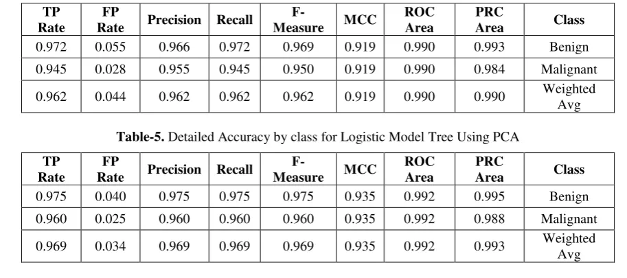
Table-4. Detailed Accuracy by class for Logistic Model Tree Using J48.

TP Rate

FP

Rate Precision Recall

F-Measure MCC

ROC Area

PRC

Area Class

0.972 0.055 0.966 0.972 0.969 0.919 0.990 0.993 Benign

0.945 0.028 0.955 0.945 0.950 0.919 0.990 0.984 Malignant

0.962 0.044 0.962 0.962 0.962 0.919 0.990 0.990 Weighted Avg

Table-5. Detailed Accuracy by class for Logistic Model Tree Using PCA

TP Rate

FP

Rate Precision Recall

F-Measure MCC

ROC Area

PRC

Area Class

0.975 0.040 0.975 0.975 0.975 0.935 0.992 0.995 Benign

0.960 0.025 0.960 0.960 0.960 0.935 0.992 0.988 Malignant

Also, Table-6 gives the values for objects of the trained Random Forest classifier.

Table-6. Values for Parameters of Trained Logistic Model Tree.

Attribute Values (using J48)

Values (using PCA)

Number of Boosting

Iterations (I) 15 4 Minimum Number of

Instances (M) 1 1

Weight Trim Beta (W) 0.0 0.0

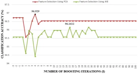
The classifier depends on three variables which are number of boosting iterations (I), Minimum number of instances (M) and weight trim beta (W). The value of the parameter “Number of boosting iterations [I]” changes with respect to the filter. Other parameters remain constant for both J48 and PCA. The variation of these parameters vs. the algorithms classification accuracy is plotted in Figure 2-4 respectively

Figure-2. Values of Number of Boosting Iterations Vs Classification accuracy.

Varying the parameter titled ‘Number of boosting iterations’ (Figure-2) from -3to 100. The curve corresponding to PCA remains constant upto the step ‘0’ then drops in step of ‘1’. However, on further iterations the classification accuracy increases to a maximum at ‘4’. On the other hand, the curve corresponding to J48 remains steady up to‘0’ then shows continuous fluctuations

Figure-3. Minimum Number of Instances against Classification accuracy.

Varying the parameter titled ‘Minimum number of instances’ (Figure-3) from 0 to 100, the curve corresponding to PCA gives constant classification accuracy for all values. At the same time the curve corresponding to J48 initially stays constant, progresses with minor fluctuations then attains a steady state on further iterations.

Figure-4. Weight trim Beta against Classification accuracy.

On varying the parameters ‘weight trim beta’ (Figure-4) from 0 to 1.0, both curves show a monotonically decreasing classification accuracy in steps up to ‘0.9’. Further. Beyond 0.9 gives a sudden fall in classification accuracy. However, From the above three graphs it can be concluded that the curve corresponding to PCA stood superior in classification accuracy with respect to the changes in parameters. The classifier achieved a maximum classification accuracy of 96.929% after feature selection using Principal Component Analysis (PCA).

4.2 Classification using Random forest tree

Tables 7 & 8 shows the confusion matrices of Random forest classifier using J48 & PCA for selecting features respectively.

Table-7. Confusion Matrix of Random Forest Using J48.

Classified as Benign Malignant

Benign 310 10

Malignant 8 193

Table-8. Confusion Matrix of Random Forest Using PCA.

Classified as Benign Malignant

Benign 308 12

Malignant 10 191

So, it can be concluded that the number of correctly classified instances are greater while using J48 for selecting features.

Table-9 shows the stratified cross validation details of the classifier. Tables 10 & 11 display the detailed accuracy by class for both J48 and PCA respectively.

Table-9. Cross Validation of Random Forest.

Feature Selection using J48 Feature Selection using PCA

Correctly classified instances incorrectly classified instances

503 18

499 22

Kappa statistic 0.9272 0.9111

Mean absolute error 0.0735 0.052

Root mean squared error 0.1826 0.1845

Relative absolute error 15.4999% 10.9615 %

Root relative squared error 37.5109% 37.8959 %

Total number of instances 521 521

Table-10. Detailed Accuracy by class for Random Forest Using J48.

TP Rate

FP

Rate Precision Recall

F-Measure MCC

ROC Area

PRC

Area Class

0.963 0.050 0.969 0.963 0.966 0.911 0.986 0.987 Benign

0.950 0.038 0.941 0.950 0.946 0.911 0.986 0.971 Malignant

0.958 0.045 0.958 0.958 0.958 0.911 0.986 0.981 Weighted Avg

Table-11. Detailed Accuracy by class for Random Forest Using PCA.

TP Rate

FP

Rate Precision Recall

F-Measure MCC

ROC Area

PRC

Area Class

0.969 0.040 0.975 0.969 0.972 0.927 0.990 0.994 Benign

0.960 0.031 0.951 0.960 0.955 0.927 0.990 0.982 Malignant

0.965 0.037 0.966 0.965 0.965 0.927 0.990 0.989 Weighted Avg

Also, Table-12 gives values for objects of the trained Random Forest classifier.

Table-12. Values for Parameters of Trained Random Forest.

Attribute Values (using J48)

Values (using PCA)

Number of Iterations (I) 25 14

Number of Features (M) 1 0

Seed (S) 11 1

The classifier depends on three parameters which are number of iterations (I), number of features (K) and seed (S). For These two filters, the classifier attains maximum classification accuracy with different values of the parameter. The variation of these parameters vs. the algorithms classification accuracy is plotted in Figures 5-7 respectively.

Figure-5. Number of Iterations against Classification accuracy.

maximum accuracy then displays a monotonic decrease in the classification accuracy

Figure-6. Number of Features against Classification accuracy.

Varying the parameter titled ‘Number of features (K)’ (Figure-6) from 0 to 100. in steps of ‘1’ caused a slight drop in classification accuracy for the curve corresponding to PCA. However, it improves the classification accuracy in step of’2’ which was maintained. But the curve for J48 attained maximum in step of ‘1’. Further moves in a fluctuational manner then reached the steady state in step ‘7’

Figure-7. Seed Vs Classification accuracy.

Varying the parameter ‘seed’ (Figure-7) from 1 to 100. Both the curves move with continuous ups and

downs. The curve of PCA starts from maximum classification accuracy then get fluctuations with respect to the changes of parameters. But in the other case the curve attains the maximum value in the middle of the iterations. However, the curves corresponding to J48 displays higher classification accuracy in the above three graphs. The classifier achieved a maximum classification accuracy of 96.5451% after selecting features using J48.

4.3 Classification using Hoeffding tree

Tables 13 & 14 shows the confusion matrices for the classifier using J48 and PCA are filters.

Table-13. Confusion Matrix of Hoeffding tree Using J48.

Classified as Benign Malignant

Benign 308 12

Malignant 9 192

Table-14. Confusion Matrix of Hoeffding tree Using PCA.

Classified as Benign Malignant

Benign 309 11

Malignant 7 194

From Confusion matrix (Table-13), it can be point out that 308/320 samples were correctly classified as Benign, 192/201 samples were correctly classified as Malignant. Similarly, from Table-14 it can be noted that 309/320samples were correctly classified as Benign; 194/201samples were correctly classified as Malignant. So, it can be observed that the number of correctly classified instances are greater while using PCA for selecting features.Table 15shows the stratified cross validation details of the classifier. Tables 16 & 17 displays the detailed accuracy by class for both J48 and PCA respectively.

Table-15. Cross Validation of Hoeffding tree.

Feature Selection using J48 Feature Selection using PCA

Correctly Classified Instances Incorrectly Classified Instances

500 21

503 18

Kappa statistic 0.9152 0.9274

Mean absolute error 0.0435 0.059

Root mean squared error 0.1953 0.1843

Relative absolute error 9.1671% 12.4402%

Root relative squared error 40.1163% 37.856 %

Table-16. Detailed Accuracy by class for Hoeffding Tree Using J48.

TP Rate

FP

Rate Precision Recall

F-Measure MCC

ROC Area

PRC

Area Class

0.963 0.045 0.972 0.963 0.967 0.915 0.990 0.994 Benign

0.955 0.038 0.941 0.955 0.948 0.915 0.988 0.971 Malignant

0.960 0.042 0.960 0.960 0.960 0.915 0.989 0.986 Weighted Avg

Table-17. Detailed Accuracy by class for Hoeffding Tree Using PCA.

TP Rate

FP

Rate Precision Recall

F-Measure MCC

ROC Area

PRC

Area Class

0.966 0.035 0.978 0.966 0.972 0.927 0.965 0.974 Benign

0.965 0.034 0.946 0.965 0.956 0.927 0.965 0.929 Malignant

0.965 0.035 0.966 0.965 0.966 0.927 0.965 0.957 Weighted Avg

Also, Table-18 gives values for objects of the trained Random Forest classifier

Table-18. Values for Parameters of Trained Hoeffding Tree.

Attribute Values (using J48)

Values (using PCA)

Hoeffding Tie Threshold 0.1 0.1

(H)

The classifier depends on the parameter Hoeffding Tie Threshold (H). The value of this parameter is same while applying both filters. For this value of parameter the classifier attains maximum accuracy. The variation of this parameter vs. the algorithms classification accuracy is plotted in Figure-10.

Figure-8. Hoeffding Tie Threshold Vs Classification accuracy.

Varying the parameter titled ‘Hoeffding tie threshold (H)’ (Figure-10) from 0.1 to 1.0, the classification accuracy remains constant when features are selected using PCA. On the other hand, the curve corresponding to J48 originates from maximum value of classification accuracy. Further, caused a sudden fall in the

next step ‘0.15’, then improves toa constant value. The classifier achieved a maximum classification accuracy of 96.5451% after selecting features by PCA. Logistic model Tree stood up with highest classification accuracy.

5. CONCLUSIONS

By implementing data mining techniques, early diagnosis of breast cancer is practical. The prominent features that can be used for prognosis should be extracted for this purpose. Analyzing the developed patterns by Principal Component Analysis (PCA) and J48, it is easier to select prominent features which allow the effective, early and precise diagnosis. The research for a powerful Filter-classifier combination for breast cancer diagnosis ends with the combination of Principal component Analysis (PCA) as filter and Logistic Model Tree (LMT) classifier. So, it is inspiring to conclude that the implementation of Principal component analysis (PCA) for feature reduction and Logistic Model Tree (LMT) for classification is a suitable pair for Breast cancer detection. The Future researches can be executed by choosing distinct algorithms, varying the parameters and by applying distinct filters to produce a generalized result.

REFERENCES

Ai-ling Teh. 2010. A novel principal component analysis method for identifying differentially expressed gene signatures.Graduate Theses and Dissertations. 11394, Iowa State University.

Arvind Kumar, Parminder Kaur, Pratibha Sharma. 2015. A Survey on Hoeffding Tree Stream Data Classification Algorithms. CPUH-Research Journal. 1(2): 28-32, ISSN (Online): 2455-6076.

Dr Prof. Neeraj, Sakshi Sharma, Renuka Purohit, Pramod Singh Rathore. 2017. Prediction of Recurrence Cancer using J48 Algorithm. Proceedings of the 2nd International Conference on Communication and Electronics Systems, (ICCES 2017) IEEE Explore Compliant - Part Number: CFP17AWO-ART, ISBN: 978-1-5090-5013-0.

Eesha Goel. Er. Abhilasha. 2017. Random Forest: A Review. International Journal of Advanced Research in Computer Science and Software Engineering. 7(1), ISSN: 2277 128X.

Elangovan M., Babu Devasenapati S., Sakthivel N. R., Ramachandran K. I. 2011. Evaluation of expert system for condition monitoring of a single point cutting tool using principle component analysis and decision tree algorithm. Expert Systems with Applications. 38, 4450-4459.

Francisco Castells, Pablo Laguna, Leif Sornmo, Andreas Bollmann, Jos´e Millet Roig. 2007 Principal Component Analysis in ECG Signal Processing. EURASIP Journal on Advances in Signal Processing, Article ID 74580, Vol. 2007.

Hamsagayathri P., Sampath. 2017. Decision Tree Classifiers for Classification of Breast Cancer. International Journal of Current Pharmaceutical Research. 9(2), ISSN- 0975-7066.

Jegadeeshwaran R., Sugumaran V. 2013. Comparative study of decision tree classifier and best first tree classifier for fault diagnosis of automobile hydraulic brake system using statistical features. Measurement. 46, 3247-3260.

Joshuva A., Sugumaran V. 2018. A Study of Various Blade Fault Conditions on a Wind Turbine Using Vibration Signals through Histogram Features. Journal of Engineering Science and Technology. 13(1): 102-121.

Jyotismita Talukdar; Dr. Sanjib, Kr. Kalit. 2015. Detection of Breast Cancer using Data Mining Tool (WEKA). International Journal of Scientific & Engineering Research. 6(11), November, 1124 ISSN 2229-5518.

Konstantina Kourou, Themis P. Exarchos, Konstantinos P. Exarchos, Michalis V. Karamouzis, Dimitrios I. Fotiadis. 2015. Machine learning applications in cancer prognosis and prediction. Computational and Structural Biotechnology Journal. 13, 8-17.

Liton Chandra Paul, Abdulla Al Suman, Nahid Sultan. 2013. Methodological Analysis of Principal Component Analysis (PCA) Method. IJCEM International Journal of Computational Engineering & Management. 16(2) 2230-7893.

Manju. B. R., Joshuva A., Sugumaran V. 2018. A Data Mining Study for Condition Monitoring On Wind Turbine Blades Using Hoeffdingtree Algorithm through Statistical and Histogram Features. International Journal of

Mechanical Engineering and Technology (IJMET), 9(1): 1061-1079, Article ID: IJMET_09_01_113.

Nagesh Shukla, Markus Hagenbuchner, Khin than Win, Jack Yang. 2018. Breast cancer data analysis for survivability studies and prediction. Computer Methods and Programs in Biomedicine. 155(2018): 199-208.

Novakovic J., Rankov S. 2011. Classification Performance Using Principal Component Analysis and Different Value of the Ratio R. Int. J. of Computers, Communications & Control, ISSN 1841-9836, E-ISSN 1841-984, 2: 317-3271.

Philip K. Chan, Richard P. Lippman. 2006. Machine Learning for Computer Security. Journal of Machine Learning Research. 7, 2669-2672.

Ravikumar S.; Ramachandran K. I., Sugumaran V. 2011. Machine learning approach for automated visual inspection of machine components. Expert Systems with Applications. 38, 3260-3266.

Rebecca Jeya Vadhanam B., Mohan S., Ramalingam. V.V., Sugumaran, V. 2016. Performance Comparison of Various Decision Tree Algorithms for Classification of Advertisement and Non Advertisement Videos. Indian Journal of Science and Technology. 9(48).