Upgraded global mapping information for earth system modelling: an application to surface water depth at the ECMWF

https://doi.org/10.5194/hess-23-4051-2019 © Author(s) 2019. This work is distributed under the Creative Commons Attribution 4.0 License.

Upgraded global mapping information for earth system modelling:

an application to surface water depth at the ECMWF

Margarita Choulga1, Ekaterina Kourzeneva2, Gianpaolo Balsamo1, Souhail Boussetta1, and Nils Wedi1 1_{Research Department, European Centre for Medium-Range Weather Forecasts (ECMWF), Reading, RG2 9AX, UK} 2_{Research Department, Finnish Meteorological Institute (FMI), Helsinki, 00560, Finland}

Correspondence:Margarita Choulga ([email protected]) Received: 13 May 2019 – Discussion started: 24 May 2019

Accepted: 21 August 2019 – Published: 1 October 2019

Abstract.Water bodies influence local weather and climate, especially in lake-rich areas. The FLake (Fresh-water Lake model) parameterisation is employed in the Integrated Fore-casting System (IFS) of the European Centre for Medium-Range Weather Forecasts (ECMWF) model which is used operationally to produce global weather predictions. Lake depth and lake fraction are the main driving parameters in the FLake parameterisation. The lake parameter fields for the IFS should be global and realistic, because FLake runs over all the grid boxes, and then only lake-related results are used further. In this study new datasets and methods for generat-ing lake fraction and lake depth fields for the IFS are pro-posed. The data include the new version of the Global Lake Database (GLDBv3) which contains depth estimates for un-studied lakes based on a geological approach, the General Bathymetric Chart of the Oceans and the Global Surface Wa-ter Explorer dataset which contains information on the spa-tial and temporal variability of surface water. The first new method suggested is a two-step lake fraction calculation; the first step is at 1 km grid resolution and the second is at the resolution of other grids in the IFS system. The second new method involves the use of a novel algorithm for ocean and inland water separation. This new algorithm may be used by anyone in the environmental modelling community. To as-sess the impact of using these innovations, in situ measure-ments of lake depth, lake water surface temperature and ice formation/disappearance dates for 27 lakes collected by the Finnish Environment Institute were used. A set of offline ex-periments driven by atmospheric forcing from the ECMWF ERA5 Reanalysis were carried out using the IFS HTESSEL land surface model. In terms of lake depth, the new dataset shows a much lower mean absolute error, bias and error

stan-dard deviation compared to the reference set-up. In terms of lake water surface temperature, the mean absolute error is re-duced by 13.4 %, the bias by 12.5 % and the error standard deviation by 20.3 %. Seasonal verification of the mixed layer depth temperature and ice formation/disappearance dates re-vealed a cold bias in the meteorological forcing from ERA5. Spring, summer and autumn verification scores confirm an overall reduction in the surface water temperature errors. For winter, no statistically significant change in the ice forma-tion/disappearance date errors was detected.

1 Introduction

northern Russia and Siberia. Lakes influence local weather conditions and local climate. For example, during freezing and melting the lake surface radiative and conductive prop-erties and the latent and sensible heat released to the atmo-sphere change dramatically, resulting in a completely differ-ent surface energy balance (Eerola et al., 2010; Mironov et al., 2010a; Samuelsson et al., 2010; Rontu et al., 2012). Lake Ladoga in Russia can generate low clouds which lead to an increase in 2 m temperatures of up to 10◦C in neighbour-ing Finland (Eerola et at., 2014). The Great Lakes in the USA intensify winter snow storms (Hjelmfelt, 1990; Notaro et al., 2013; Vavrus et al., 2013). During summer in the boreal zone lakes usually cause a decrease in the amount of precip-itation (Samuelsson et al., 2010). The African Lake Victo-ria generates night convection with intensive thunderstorms, which leads to the deaths of thousands of fishermen every year (Thiery et al., 2015, 2017). Lakes can also influence global climate by affecting the carbon cycle through carbon dioxide (CO2) and methane (CH4) emissions (Tranvik et al., 2009, Stepanenko et al., 2016). Small shallow thermokarst lakes located at boreal and Arctic latitudes in the permafrost thaw area are rich in organic matter from permafrost erod-ing into anaerobic lake bottoms (Walter et al., 2006; Stepa-nenko et al., 2012), which affect the CH4 budget, being as large as the CO2budget for these lakes (Walter et al., 2007). This type of lake is the most common one (representing ap-proximately 77 % of the lakes globally) and in general has a small surface area (0.002–0.01 km2) and a big surface-to-volume ratio. These shape characteristics are important as carbon dioxide and methane degassing takes place through the lake’s surface (Borre, 2014; Verpoorter et al., 2014).

The effect of lakes is handled in numerical weather pre-diction (NWP) and climate models through parameterisa-tion, which needs information on the locations of the lakes and their morphological characteristics. However, their rep-resentation within global models may be problematic be-cause 90 million of the world’s lakes range between 0.002 and 0.01 km2in size (Borre, 2014; Verpoorter et al., 2014). To date, the majority of the morphological parameters of these lakes have not been measured, not to mention con-stantly monitored. Reasons for this include that (i) most of these lakes are too small and common to have specially ded-icated measuring campaigns or that (ii) they are situated in very remote and hard-to-reach areas. In NWP lakes with ar-eas smaller than the model grid-box size are considered to be sub-grid features. For example, the high-resolution ver-sion of the Integrated Forecasting System (IFS) model at the European Centre for Medium-Range Weather Forecasts (ECMWF) uses a grid spacing of approximately 9 km. In this configuration lakes with a surface area of less than 81 km2 are considered to be sub-grid. The effect of both sub-grid and resolved lakes in NWP and climate modelling is taken into account through parameterisation. However, to represent the sub-grid lakes, the lake fraction (relative to the model grid size) is needed.

At the ECMWF, the lake parameterisation was introduced in 2015 by including the Fresh-water Lake model, FLake, in the IFS (Mironov et al., 2006, 2010b, 2012; Mironov, 2008). To represent surface heterogeneity, the Tiled ECMWF Scheme for Surface Exchanges over Land incorporating land surface hydrology (HTESSEL) was used. This computes sur-face turbulent fluxes (of heat, moisture and momentum) and skin temperature over different tiles (vegetation, bare soil, snow, interception and water) and then calculates an area-weighted average for the grid box to couple with the atmo-sphere (Balsamo et al., 2012; IFS Documentation, 2017). A new tile, representing lakes, reservoirs, rivers and coastal wa-ters, was introduced (Dutra et al., 2010; IFS Documenta-tion, 2017; see http://www.flake.igb-berlin.de/papers.shtml, last access: 23 September 2019) in HTESSEL based on the FLake model. Currently FLake only accurately represents freshwater lakes, but in the future its large research com-munity plans to also include representation of saline water. FLake is a one-dimensional model, which uses an assumed shape for the lake temperature profile including the mixed layer (uniform distribution of temperature) and the thermo-cline (its upper boundary located at the mixed layer bottom and the lower boundary at the lake bottom). The model also contains an ice module, a snow module and a bottom sedi-ments module. The ice albedo is dependent on the temper-ature at the ice upper surface and is lower in spring, dur-ing the meltdur-ing period; see IFS Documentation (2017) for more details. At present FLake runs in the IFS with no bot-tom sediment and snow modules (snow accumulation over ice is not allowed and snow parameters are used only for albedo purposes). In the implementation in IFS lake ice can be fractional within a grid box with inland water (10 cm of ice means 100 % of a grid box or tile is covered with ice; 0 cm of ice means 100 % of the grid box is covered by wa-ter; in between a linear interpolation is applied) (Manrique-Suñén et al., 2013). At present, the water balance equation is not included for lakes and the lake depth and surface area are kept constant in time (IFS Documentation, 2017). FLake also requires the lake fraction, Frlake, and lake depth (prefer-ably bathymetry), Dwater, and lake initial conditions. Dwater is the most important external parameter that FLake uses. Note that the IFS model is a global spectral NWP model, which uses different set-ups for its climate, ocean and ensem-ble run calculations and different horizontal resolutions. Cur-rently, the highest operational resolution is 9 km (Tco1279; the resolution of the IFS is indicated by specifying the spec-tral truncation prefixed by the acronym Tco for triangular– cubic–octahedral). It is important that lake parameterisation is consistent with other external model parameters on differ-ent resolution grids.

changes to inland water bodies and major depth changes to large lakes. The Dwaterfield should be updated with the lat-est available information to ensure that depths are close to observed values, as overestimated depths can be blamed for cold biases in summer temperatures or lack of ice. A realistic bathymetry can be obtained from new in situ measurements and high-resolution datasets and a re-evaluation of the default depths.

The aim of this research is to improve forecasts of sur-face parameters in the ECMWF’s IFS model by upgrading the lake model Frlakeand Dwater fields with newly available information. The new methods are suggested. The first new method is a two-step lake fraction calculation; the first step is at 1 km grid resolution and the second is at the resolution of other grids in the IFS system. The second new method in-volves the use of a novel algorithm for ocean and inland wa-ter separation. This includes providing consistency between lake data and other land surface fields. The impact of these innovations was studied.

The paper is organised as follows. Section 2 describes the “Data” and includes the description of the physiographic datasets used to generate the lake parameters. Section 3 dis-cusses the “Methods” applied to the datasets for both the cur-rently operational and upgraded versions. Verification of IFS simulations against in situ measurements of lake depth, lake surface water temperature and ice formation/disappearance dates, and a discussion of the results and further develop-ments, are covered in Sect. 4 on “Verification and discus-sion”. The main results, a discussion and further research guidance are covered in the “Conclusion” in Sect. 5.

2 Data

The physiographic datasets used in the IFS model to gener-ate the lake parameters are described here for both the cur-rent and upgraded versions. In addition, descriptions of the other lake-related land surface parameter datasets are given. Firstly, Frlakeis related to land use. There are a lot of regional and global ecosystem datasets such as Corine (CLC2006 technical guidelines, 2007) and Ecoclimap (Champeaux et al., 2004) that provide information on land cover types, in-cluding inland water (lakes, rivers, etc.). For land cover types, ECMWF uses the GlobCover 2009 global map (Bontemps et al, 2011; Arino et al., 2012), which has a nominal resolution of 300 m. This land cover map is used by many limited-area models (e.g. COSMO) and has been proven to be an accu-rate and reliable source of data for NWP modelling (Arino et al., 2012; Quaife and Cripps, 2016). GlobCover 2009 is de-rived from an automatic, regionally tuned classification of a time series of global Medium Resolution Imaging Spectrom-eter Instrument Fine Resolution (MERIS FR) mosaics for the year 2009. It consists of a global land cover map on a Plate-Carree (WGS84 ellipsoid) projection covering the Earth. Its legend is compatible with the GLC2000 (Bartholome and

Belward, 2005) global land cover classification and accounts for 22 land cover classes defined with the United Nations (UN) Land Cover Classification System (LCCS). A 23rd class (coded as “230”) has been added to the final legend to account for pixels with no data (Bontemps et al, 2011). The GlobCover 2009 land cover map is available from 60◦S to 85◦N but contains only one “water” cover type and hence does not distinguish between ocean (sea) and inland water bodies (lakes, rivers, etc.).

Over polar regions, for the land cover map ECMWF uses the high-resolution Radarsat Antarctic Mapping Project (RAMP) digital elevation model (DEM) Version 2 (RAMP2) data (Liu et al., 2015) for Antarctica. These data are on a 1 km (3000) grid in polar stereographic coordinates (IFS Doc-umentation, 2017) and are provided as raw binary (the only values are 0=water and 1=land). In the Arctic, north of 85◦_{N, no land is assumed.}

For the upgrade of lake location in selected places, the Digital map database of Iceland and Global Surface Wa-ter Explorer data are used. National Land Survey of Ice-land are constantly reviewing and processing the Digital map database of Iceland (IS 50V). It is based on a variety of sources and data such as GPS tracking for roads, aerial photographs, SPOT-5 satellite images and data from other agencies and municipalities. IS 50V consists of eight lay-ers, including hydrology and coastline. Layers are presented in conical Lambert projection (the reference is ISN93 or ISN2004). For our purposes, only coastline and hydrology layers are used to update water distribution for Iceland; these were processed by the Icelandic Meteorological Office (Bolli Palmason and Ragnar Heiðar Þrastarson, personal communi-cation, 2018).

years in which reliable observations were obtained. These are the following.

(0) No water – water was not detected in this place. (1) Permanent – unchanging permanent water surfaces. (2) New permanent – conversion of a no-water place into a

permanent water place.

(3) Lost permanent – conversion of a permanent water place into a no-water place.

(4) Seasonal – unchanging seasonal water surfaces. (5) New seasonal – conversion of a no-water place into a

seasonal water place.

(6) Lost seasonal – conversion of a seasonal water place into a no-water place.

(7) Seasonal to permanent – conversion of seasonal water into permanent water.

(8) Permanent to seasonal – conversion of permanent water into seasonal water.

(9) Ephemeral permanent – no-water places replaced by permanent water that subsequently disappeared within the observation period.

(10) Ephemeral seasonal – no-water places replaced by sea-sonal water that subsequently disappeared within the observation period.

(255) No data – no reliable observations were obtained. This map is used to upgrade only certain geographical re-gions (i.e. Australia, Aral Sea, Alqueva Reservoir).

The lake depth is specified according to the Global Lake DataBase, v1 and v3 (Kourzeneva, 2010; Choulga et al., 2014), for operational and upgraded versions respectively. In 2008 GLDBv1 was developed for implementation in lake parameterisation schemes in NWP and climate modelling (Kourzeneva, 2010). GLDBv1 uses

i. the mean depth for individual lakes (∼13 000 lakes) from different regional databases,

ii. the global lake mask created from the Ecoclimap2 ecosystem dataset (Champeaux et al., 2004), and iii. bathymetry data for 36 large lakes from ETOPO1

(Amante and Eakins, 2009) and digitised navigation and topographic maps.

To combine individual lake depth data with a raster cover map, an automatic probabilistic mapping method is used; see Kourzeneva et al. (2012) for more information. The re-sult was a global lake depth dataset on a 3000 (∼1 km) grid.

When there was a lake on the map but its depth value was un-known from the individual lake dataset, the “default” depth of 10 m was used. GLDBv1 is used in the IFS operational set-up. In GLDB later versions, the “default” depth was the main subject of study. GLDBv1 was upgraded with indirect mean depth estimates, depending on the geological origin of the lake. The geological approach, used for the depth esti-mation of uninspected freshwater lakes, assumes that water bodies of the same origin and the same age should have sim-ilar morphological parameters; see Choulga et al. (2014) for more information. An innovative algorithm, which combined information about lake location and morphological param-eters, and surface geological and tectonic information, was developed and applied. Globally 374 regions (141 for the bo-real climate zone and 233 for the rest of the globe) with a homogeneous geological origin of lakes were outlined. The typical lake depth values were derived from (1) the individ-ual lake dataset and global gridded lake depth map statistics, (2) expert judgement, and (3) lists with different lake types, exceptional for the region with the same lake origin. The re-cent version of the dataset is GLDBv3. Its main differences from GLDBv1 are the following:

i. increase in the individual lake list by∼1500 lakes; ii. addition of extra bathymetry data for all navigable and

most non-navigable Finnish lakes;

iii. addition of indirect mean depth estimates based on lake geological origin;

iv. use of the derived analytical equations to define the lake mean depth from the lakes’ area and boreal zones’ cli-mate type; see Choulga et al. (2014) for more detailed information;

v. introduction of freshwater/saline lake differentiation: the “default” depth for freshwater lakes is set to 10 m, and for saline lakes it is 5 m; and

vi. introduction of two lists with exceptions: artificial lakes (reservoirs) with unknown depths and crater (caldera) lakes with the “default” depths of 10 and 50 m respec-tively.

Verification of indirect depth estimates (based on geologi-cal origin) against new observations for 353 Finnish lakes showed 52 % bias reduction (from 5.4 m in GLDBv1 to 2.6 m in GLDBv3) and 34 % RMSE reduction (from 6.1 m in GLDBv1 to 4.0 m in GLDBv3); improvements in the depth estimates are proven to be statistically significant. In this study GLDBv3 is used to upgrade the IFS lake information.

(∼2 km). ETOPO1 consists of regional and global datasets and bathymetry estimates from satellite altimetry for unsur-veyed ocean areas. Horizontal and vertical data of the model are WGS 84 geographic and “sea level” accordingly.

The upgraded bathymetry for the Caspian Sea, the Azov Sea and the ocean is from the General Bathymetric Chart of the Oceans (GEBCO) (Weatherall et al., 2015). Published in 2014, GEBCO is a global terrain model for ocean and land with a 3000 (∼1 km) global grid of elevations. It is largely generated by combining new versions of regional bathymet-ric compilations from the International Bathymetbathymet-ric Chart of the Arctic Ocean, the International Bathymetric Chart of the Southern Ocean, the Baltic Sea Bathymetry Database, and data from the European Marine Observation and Data net-work bathymetry portal, quality-controlled ship depth sound-ings with interpolation between sounding points guided by satellite-derived gravity data. The dataset is accompanied by auxiliary data, where each cell’s value is identified based on actual depth values or predicted ones.

3 Methods 3.1 Current status

The IFS is a global model, and according to its design, lake parameterisation runs on each surface grid point, whether the simulation results in this point are used later or not. Indepen-dently of the resolution, missing values are not allowed to ease the interoperability of the output at diverse spatial reso-lutions of the IFS model.

The main physiographic fields that govern use of all land-surface parameterisation results in the IFS are the land frac-tion (Frland) and the corresponding land–water binary mask (LWM, 0=water and 1=land). Frlandprovides information about the land and water (oceans, seas, lakes, rivers, etc.) fraction in each model grid box of the underlying surface. In the IFS, the model grid box is land-dominated if more than 50 % of the actual surface is land (Manrique-Suñén et al., 2013) (i.e. Frland>50 %→ LWM=1). All sub-grid water in the land-dominating case is treated as lake wa-ter (simulated by FLake). If a grid box is wawa-ter-dominated (i.e. Frland ≤50 % →LWM=0), then extra knowledge of the water type is required, as salt ocean and predominantly freshwater lakes and rivers have different physical proper-ties and are treated with different model parameterisations. Both Frland and LWM are grid-dependent. Primarily, Frland is calculated from the land-cover maps (operationally from GlobCover 2009 and RAMP2) by aggregating the “land”-type information on a certain grid. Then the LWM is pro-duced. Note that since GlobCover 2009 does not distinguish between ocean (sea) and inland water, the LWM also does not distinguish between them.

To distinguish between ocean and inland water, a binary lake mask (LKM, 0=non-lake and 1=lake) is produced

from the LWM using a flood-filling algorithm for different resolutions and grids. The idea of this algorithm is to start from a seed somewhere in the open ocean on the LWM and let the flood-filling procedure (IFS Documentation, 2017) march through all connected water points (i.e. where LWM= 0), marking them as non-lake (i.e. with LKM=0); unmarked points with LWM=0 are not connected to the ocean and stand for the inland water bodies (i.e. LKM=1). The rea-sons for applying this method instead of using an LKM pro-duced from external sources (e.g. from GLDBv1) are the fol-lowing. Various sources of information almost always have some compatibility errors, in this case – spatial distribution errors – and inland water bodies from different inventories can have variations in location, shape and size. It is vital to have LKM consistent with LWM; otherwise, ocean water can surprisingly appear on the Tibetan Plateau. Also, a new high-resolution updated LWM appears much earlier than LKMs based on them, which are usually with lower resolution. As in NWP the quality (accuracy and reliability) of water land data is extremely important: having an up-to-date high-resolution LWM is very appealing. This leads to the necessity of an in-house algorithm to generate an LKM from the chosen LWM dataset. Issues here are grid dependency and low ac-curacy. Some lakes are very close to the sea, and especially for low resolutions, the flood-filling algorithm just fills them up as ocean. This issue was resolved by manually blocking coastal lakes. Another issue was that some narrow parts of the ocean (e.g. fjords in Norway and Greenland) were not filled up by the flood-filling algorithm (leaving them to freeze as freshwater bodies). The solution here was to use a latitude-dependent threshold for the LWM (to distinguish water from land) while using the flood-filling algorithm, with lower val-ues at mid and low latitudes and higher valval-ues at high lati-tudes (IFS Documentation, 2017). Finally, FLake results are used for the grid boxes with LWM=1 or with LWM=0 and LKM=1, using Frlake=1−Frland. This algorithm is applied separately for each IFS grid with different horizontal reso-lutions (operational (∼9 km, Tco1279), climate, ocean, and ensemble).

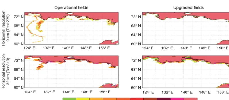
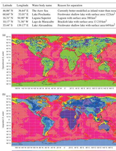
Figure 1.Combination of operational and upgraded Frlandand Frlakefields showing the remaining ocean water over Finland and north-western Russia (59–72◦N, 20–42◦E) at different horizontal resolutions; colours indicate the ocean fraction in each grid box: white – no ocean; pink – fully covered with ocean.

Figure 2.Same as Fig. 1 but over north-eastern Russia (60–74◦N, 122–163◦E).

The main disadvantage of the current ocean–inland wa-ter separating procedure is simplification of a complex coast-line (e.g. Finland, Norway) and neglect of small islands. At coarser resolution narrow land parts that separate freshwa-ter lakes and saline ocean disappear (land fraction becomes too small) and coastal lakes and wide estuaries are treated as ocean (the surface temperature is extrapolated from the sea surface temperature of the nearest ocean grid point), which can lead to no-ice conditions during winter at high latitudes or rather low temperatures and almost no diurnal cycle during summer. One example is disappearing islands that separate

water separating procedure leads to deep ocean penetration into land and/or separated ocean parts over the land at coarser resolutions. For example, Fig. 1, left column upper plot, at 9 km resolution shows neat separation of inland water and ocean, and Fig. 1, left column lower plot, at 32 km resolu-tion shows that the same water separaresolu-tion procedure leads to deep ocean penetration inland filling Lake Saimaa with salt water through pixels that became not land-dominated at coarser resolution. In addition, several inaccuracies were re-ported in inland water distribution, such as a too wet Aus-tralia and omission of Alqueva Reservoir – the biggest man-made lake in western Europe. All these features required an urgent update.

3.2 Updates

The proposed way of creating lake fields is first to create an LKM compatible with an LWM at a 1 km resolution regu-lar latitude–longitude grid, and then to interpolate both to the needed resolution and grid. This will allow us to preserve water fractions of both types at any resolution independently of Frland. Figures 1 and 2, right columns, give a quick peek at the Frlandand Frlakefield combination (remaining fractional ocean part) created with the new way at 9 km (Tco1279, up-per plots) and 32 km (Tco319, lower plots) horizontal resolu-tions over the Finland and north-western Russia (59–72◦N, 20–42◦E) and north-eastern Russia (60–74◦N, 122–163◦E) regions respectively. These plots show how use of the new ocean/inland water separating procedure prevents deep ocean penetration into land and/or separation of ocean parts over the land at coarser resolutions. The proposed methodology is designed bearing in mind quite prompt update of global ecosystem maps: new satellite-based products become freely available with higher and higher resolution more often. To ease the LKM compatibility with LWM upgrade process, the water-type separation procedure is as automated as possible. Dwater is the main parameter to drive lake parameterisation. In the IFS surface scheme FLake runs on each grid point in-dependently of the Frlake, so the Dwaterfield should be global and as realistic as possible. To achieve this, newer dataset versions, various data source compilations and innovative ap-proaches were used.

The new way of generating the LKM field was (1) to start with a 1 km LWM and (2) to create a consistent 1 km LKM, then (3) to convert a binary LKM field into a fractional Frlake field, and finally (4) to interpolate it to all IFS grids and res-olutions. In this case separation between ocean and inland water is done only once at rather high horizontal resolution (∼1 km), which still preserves a lot of coastal features but is computationally (and in a data handling sense) cheaper than the nominal resolution of GlobCover 2009 or GSWE (∼300 m and∼30 m respectively).

The first step was to aggregate the water cover from the initial GlobCover 2009 1000 map to 3000 (43200/21600 grid boxes along longitude and latitude) horizontal resolution. At

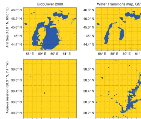
Figure 3.Water distribution from GlobCover 2009 and the GSWE Water Transitions map (only (1) permanent, (2) new permanent and (7) seasonal to permanent water classes are used); yellow colour indicates land, and dark blue indicates water.

the end of this step aggregated LWM was also corrected at certain regions where big water distribution errors were re-ported. The regions and sources are the following.

The Aral Seais an endorheic lake that used to be one of the four largest lakes in the world. In 1960 its water surface area was 68 900 km2. However, the Aral Sea is shrinking. Ac-cording to historical records this process started at least in the middle of the 18th century and was accelerated in the 1960s after massive diversion of water for cotton and rice cultiva-tion. GlobCover 2009 shows the Aral Sea for 1998 when its water surface area was 28 990 km2(less than half of its ini-tial size) (Duhovny et al., 2017); see Fig. 3, upper left plot. Nevertheless, after 1998 shrinking continued. The Aral Sea water surface area started stabilising only in 2014 at an area of 7660 km2(almost 9 times smaller than its initial size), due to the major Aral Sea recovery programme launched in 2001 by the president of Kazakhstan and supported by the World Bank (The Kazakh Miracle, 2008); see Fig. 3, upper right plot. On the updated map, an up-to-date Aral Sea water dis-tribution from GSWE replaced an outdated one from Glob-Cover 2009. Only currently present water types were used, i.e. permanent, new permanent and seasonal to permanent.

Figure 4.Water distribution for the Australian (20–30◦S, 130–140◦E) region using GlobCover 2009 and the GSWE Water Transition map with different water class combinations; permanent water stands for a combination of the (1) permanent, (2) new permanent and (7) seasonal to permanent water classes; seasonal water – (4) seasonal, (5) new seasonal and (8) permanent to seasonal; ephemeral water – (9) ephemeral permanent and (10) ephemeral seasonal; yellow colour indicates land, dark blue indicates water, and red circles indicate the locations of Lake Moondarra (upper circle) and Lake Machattie (lower circle).

Figure 5.Water distribution for Iceland using GlobCover 2009 and the Digital map database of Iceland; yellow colour indicates land, and dark blue indicates water.

Australiais the sixth largest (by total area) country in the world, with a vast number of lakes. Lakes are predominantly dry and salty, located in the flat desert regions. Excess in-land water on the GlobCover 2009 map was reported for the south-eastern part of Western Australia and the northern part of South Australia (20–30◦S, 130–140◦E), as illustrated by Fig. 4. The left plot shows the region in question on Glob-Cover 2009, with the shallow endorheic Kati Thanda–Lake Eyre (28.37◦S, 137.37◦E) in its lower right corner. This lake fills on rare occasions, only a few times a century. Here it is seen in its maximum extent. The right three plots show the same region on the GSWE Water Transitions map with different water class combinations. The combination of per-manent, new permanent and seasonal to permanent water classes reflects permanent water; see the second from left plot. This combination has almost no inland water, except the artificial Lake Moondarra (20.59◦S, 139.54◦E) and the Lake Machattie area (24.90◦S, 139.50◦E), which consists of three lakes: Mipia (usually retains water until the following flood season), Koolivoo (usually dries up by early summer) and Machattie (flooded approximately once in 3 years). Lakes in the Lake Machattie area are fresh when filled by floods but become saline as they dry out. If seasonal, new seasonal and permanent to seasonal water classes (which reflect seasonal water) are added, see the third from left plot, then the region in question has more water, yet much less than on GlobCover

2009. If ephemeral permanent and ephemeral seasonal water classes (which stay for ephemeral water) are also added (see right plot), the region in question gets even more water than on GlobCover 2009, which was reported as being too wet. To make a choice of all year-round plausible water distribu-tion for Australia, experts from Australian Nadistribu-tional Univer-sity and the Bureau of Meteorology were consulted. It was explained that there are large-scale ephemeral inundations in inland Australia, but most of them are occasional rather than seasonal (Albert van Dijk, personal communication, 2017). Based on this, it was decided to use the combination of per-manent, new permanent and seasonal to permanent water classes from the GSWE Water Transitions map as a whole year static water distribution for Australia; see Fig. 4, sec-ond from left plot. This correspsec-onds well to Water Observa-tions from Space for Australia (see https://www.nationalmap. gov.au/#share=s-eUqvVz1ZghXPUBI4ImWweurQppg, last access: 23 September 2019, and http://maps.ga.gov.au/ interactive-maps/#/theme/water/map/surfacehydrology, last access: 23 September 2019).

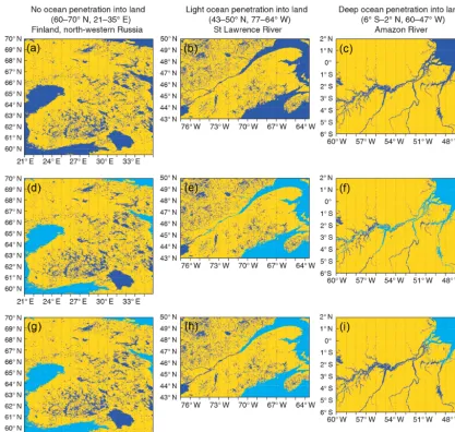
Figure 6.Phases of LWM water separation for Finland and the north-western part of Russia(a, d, g), the St Lawrence River region(b, e, h), and the Amazon River region(c, f, i): no water separation(a–c), separation with the flood-filling algorithm only (“basic” flooding,d–f) and separation with flood-filling and newly developed pixel-by-pixel water separation algorithms (“extra” flooding,g–i); yellow colour indicates land, dark blue indicates inland water (ind–fandg–i) or total water (ina–c), and light blue indicates ocean.

of Iceland provided by the Icelandic Meteorological Office and referred to as the best available for the regional source of water distribution information (Bolli Palmason and Rag-nar Heiðar Þrastarson, personal communication, 2018) was used; see Fig. 5, right plot.

Then corrected LWM produced from GlobCover 2009 (which is available from 85◦N to 60◦S) was combined with the RAMP2 dataset over Antarctica and an assumption of no land north of 85◦N. The resulting field is an updated LWM, further used for upgraded LKM creation.

The next step is the division of LWM water into inland and ocean parts. At the beginning the basic flood-filling al-gorithm was used. However, with the fine∼1 km resolution problematic regions with the deep ocean into land penetra-tion (through river estuaries) or merger of different inland

River with the Tucurui Reservoir. This Amazon River re-gion example also shows several inner water bodies merge, which makes it extremely challenging to automatically map individual lake depth with each water body, as was done in Kourzeneva et al. (2012) for mapping lake depths for GLDB. Specially for these complicated situations, when separa-tion should be based on physical and geographical rather than geometrical features, the innovative water body sepa-ration algorithm was developed and applied. In general, the algorithm allows us to separate narrow rivers or bays from large water bodies (e.g. lakes or seas). Since it is based on something more than just geometry, it contains two param-eters which depend on the resolution and complexity of the regions’ coastlines. These parameters should be defined be-forehand by relying on expert opinion (i.e. tuning parame-ters). The algorithm is pixel-by-pixel and iterative. The pa-rameters are

i. the window widthW– checking radius around the water pixel in question, defined in number of pixels (in Fig. 7 exampleW=1); and

ii. the number of iterationsL– how many times the algo-rithm must be applied over each water body (in Fig. 7 exampleL=2).

Step 0 of the new algorithm starts by working from the re-sults of the basic flood-filling algorithm. In this case the basic flood-filling algorithm should be applied so that it creates an individual water body mask, to avoid any mismatch between closely located water bodies. Then the new algorithm may be applied to each water body successively. Step 0 is shown in Fig. 7, left plot. At Step 0, each water pixel is marked with “x” if all pixels within the moving window of theW width are water, or “·” if at least one pixel in this window is non-water. Next starts the iteration phase that will be repeatedL

times. At the beginning of each iteration pixels with “·” are checked again with the moving window of theW width – if around the pixel in question there is at least one “x” pixel, it is marked as “··”; see Fig. 7, second from left plot. At the end of each iteration all “··” pixels are changed into “x” and the next iteration starts if required; see Fig. 7, third from left plot. At the end of the iteration phase the considered water body will be divided into several ones; see Fig. 7, right plot – “x” pixels will mark the main part of the water body and “·” pixels will mark the narrow rivers or bays. We applied this algorithm to separate automatically large rivers from the ocean – to stop deep penetration of the salt ocean into the land. The W andLparameters are regionally and grid de-pendent. If they are unsuccessfully defined or the coastal line is too complicated, the negative side-effect of the algorithm will appear – erroneous separation of fjords and bays from the ocean (e.g. in Norway, northern Canada, Greece and on the western coast of the USA). To stay on the safe side all the separated water bodies with the area less than 500 km2were converted back to ocean. To minimise the tuning process, the

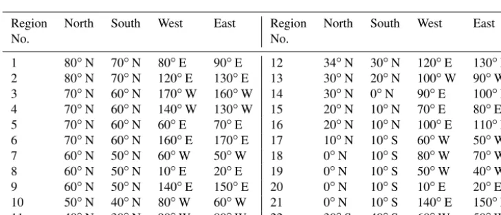
new algorithm was applied only for the specific geographical locations, where big river estuaries and lagoon-type freshwa-ter lakes are situated; see Table 1. For the upgradeL=2 and

W=3 were used. Figure 6, lower row plots, show results of basic flood-filling and newly developed pixel-by-pixel water separation algorithms use. The left plot in this row shows the region of Finland and the north-western part of Russia, which looks the same as with use of the basic flood-filling algorithm only, because this region has no big river estuaries. The mid-dle plot in the lower row shows the region of the St Lawrence River with neat separation of the freshwater river and saline ocean next to Orleans Island in Quebec (Île d’Orléan). The right plot in the lower row shows the region of the Amazon River with the realistic separation of the ocean and river es-tuary.

The final step in the LWM water separation is the visual check of the significant freshwater coastal lagoons and lakes over the globe, in case some separating islands or spits are missing on the initial ecosystem map. Also, some water bod-ies such as the Azov Sea and the Caspian Sea are better repre-sented as inland water than ocean due to the current features of the IFS. This leads to a list of exceptional water bodies (see Table 2), which were manually separated from the ocean (the Caspian Sea is marked as a lake automatically), and creation of an updated LKM.

The upgrade of the Dwater field concluded in combina-tion of all the most up-to-date reliable high-resolucombina-tion global datasets, which are GLDBv3, ETOPO1 and GEBCO. Infor-mation from GLDBv3 is used for the mean depth of the in-land water bodies, bathymetry of 36 large lakes and the ma-jority of Finnish lakes, ETOPO1 is used for the Great Lakes, and GEBCO is used for the Azov Sea, the Caspian Sea and the ocean bathymetry. The “default” 25 m depth was substi-tuted with depth estimates based on a geological approach (Choulga et al., 2014), which was implemented all around the globe. In rare cases where the geological approach had no value, the “default” depth of 10 m was used. Figure 8 shows the Dwaterfield at 9 km horizontal resolution (Tco1279): the upper plot is the operational version, the lower plot the new version. On average, all depths became shallower as the “de-fault” depth of 25 m in the operational version was substi-tuted with more realistic values.

Figure 7.Steps of the pixel-by-pixel water separation algorithm.L– number of iterations (hereL=2);W– window width (hereW=1);

·– water grid box has not only water points in its checking window; x – water grid box has only water points in its checking window;··– water grid box has at least one x in its checking window; yellow colour indicates land, and dark blue indicates water.

Table 1.List of geographical locations for the water pixel-by-pixel separation algorithm application.

Region North South West East Region North South West East

No. No.

1 80◦N 70◦N 80◦E 90◦E 12 34◦N 30◦N 120◦E 130◦E 2 80◦N 70◦N 120◦E 130◦E 13 30◦N 20◦N 100◦W 90◦W 3 70◦N 60◦N 170◦W 160◦W 14 30◦N 0◦N 90◦E 100◦E 4 70◦N 60◦N 140◦W 130◦W 15 20◦N 10◦N 70◦E 80◦E 5 70◦N 60◦N 60◦E 70◦E 16 20◦N 10◦N 100◦E 110◦E 6 70◦N 60◦N 160◦E 170◦E 17 10◦N 10◦S 60◦W 50◦W 7 60◦N 50◦N 60◦W 50◦W 18 0◦N 10◦S 80◦W 70◦W 8 60◦N 50◦N 10◦E 20◦E 19 0◦N 10◦S 50◦W 40◦W 9 60◦N 50◦N 140◦E 150◦E 20 0◦N 10◦S 10◦E 20◦E 10 50◦N 40◦N 80◦W 60◦W 21 0◦N 10◦S 140◦E 150◦E 11 40◦N 30◦N 90◦W 80◦W 22 30◦S 40◦S 60◦W 50◦W

considered a continuous field (values change smoothly from point to point). For aggregation of the inland water body depths, the mode is used. The mode is calculated for each type of depth datum separately and the non-zero value with the highest priority is used as an aggregated grid-box depth; the highest priority is given to the value calculated only from the in situ measurement, the second to the value calculated only from the depth indirect estimates, and the lowest to the “default” 10 m depth. This helps to preserve the measured values at rather high resolutions where the lake effect is most pronounced.

4 Verification and discussion

Upgraded lake-related fields must be tested prior to opera-tional implementation, as inland water bodies can have sig-nificant impact on local climate and weather in terms of 2 m temperature: over 1 K (Balsamo et al., 2012) and up to 10 K (Eerola et at., 2014) respectively. FLake prognostic variables

are the mixed-layer temperatureTML, the mixed-layer depth, the bottom temperature, the mean temperature of the total water column, the shape factor, the temperature at the ice upper surface, and the ice thickness (IFS Documentation, 2017). Verification is performed in terms ofTMLand the ice formation/disappearance dates. Modelling results are verified against in situ measurements of lake water surface tempera-ture and ice formation/disappearance dates recorded by the Data and Information Centre of the Finnish Environment In-stitute (SYKE).

4.1 Model experiment set-up and verification methods

Table 2.List of the exceptional water bodies for manual separation from the ocean.

Latitude Longitude Water body name Reason for separation

46.06◦N 36.64◦E The Azov Sea Currently better modelled as inland water than ocean 68.66◦N 53.01◦E Lake Peschanka Freshwater shallow lake with surface area 122 km2 16.31◦N 94.90◦W Laguna Superior Lagoon with surface area 380 km2

10.17◦N 71.56◦W Lago de Maracaibo Brackish lake with surface area 13 210 km2 35.44◦S 139.17◦E Lake Alexandrina Freshwater shallow lake with surface area 649 km2

Figure 8.Operational(a)and new(b)depth fields at 9 km horizontal resolution (Tco1279); depth values in metres.

ice melting in spring 2010. Experiments run with the IFS CY43R3 model on the triangular cubic octahedral grid with the high horizontal resolution∼9 km (i.e. Tco1279), in the surface offline mode (i.e. no feedback of the surface to the atmosphere). For the forcing, the lowest model-level vari-ables were taken from the newly available ERA5 reanalysis (C3S, 2017). In ERA5, the lake parameterisation is included in the model. The experiments GTZPOPR(red in all figures)

and GTZLNEW(blue in all figures) used operational and up-graded Frlakeand Dwatervalues respectively.

distribution. For the Kruskal–Wallis test, data from all com-pared groups are combined, sorted ascending and ranked; equal values are assigned with their mean rank. The Kruskal– Wallis test statisticHis

H= 12

N (N+1) K X

k=1 h

nk Rk−R 2i

, (1)

whereKis the number of groups,nk is the sample volume for group k,N is the total volume of all groups combined,

N =

K P

k=1

nk,Rk is the average rank of groupk, andRis the average rank of combined groupsR=N+1

2 . To estimate the statistical significance,H is compared with a critical value

χ2for (K−1) groups with the significance levelα(if not stated differently,α=0.05). IfH > χ2, then differences be-tween groups are statistically significant.

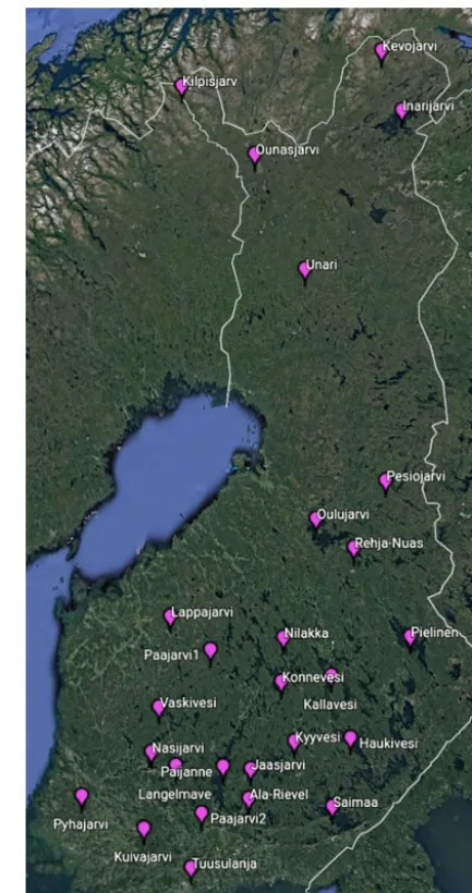
In situ SYKE data. SYKE is responsible for producing, storing and distributing Finland’s national environmental in-formation and spatial data (SYKE, 2017). SYKE operates more than 30 regular lake and river water temperature mea-surement sites over Finland. In situ lake water surface tem-perature measurements and on-shore observations of the lake visible area freeze-up/break-up dates collected by SYKE are used for the model verification. The water temperature is measured every morning during the ice-free season at 08:00 local time, close to the shore, at 20 cm below the water surface (Rontu et al., 2012, Kheyrollah Pour et al., 2017). Temperature measurements and ice formation/disappearance dates from 27 lakes for 2010–2014 are used for verification. Locations of the measurement points are shown in Fig. 9.

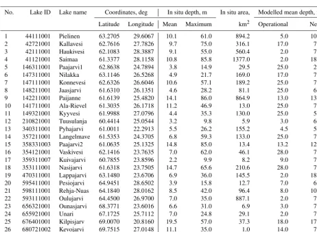
The main morphological properties of lakes are given in Table 3 and Fig. 10. This table also contains Dwater values from the model grid. Differences between in situ depth mea-surements and Dwatervalues from the model are due to hori-zontal resolution: the in situ depth values are from point mea-surements and the model depth values are from aggregated 9 by 9 km grid boxes. During the Dwater upgrade it was noted that Lake Saimaa has an incorrect mean depth (18.0 m in-stead of 10.8 m); correction is planned during the next up-grade.

Comparison between the operational and upgraded fields, considering the error as a difference between in situ and mod-elled values, shows that for 27 selected lake sites even with 9 km resolution the upgraded Dwater values have 25.4 times lower bias (−0.2 m instead of−4.8 m), 3.4 times lower MAE (2.4 m instead of 8.2 m) and 2.7 times lower SD (3.6 m in-stead of 9.7 m). Changes are statistically significant. 4.2 Model verification results

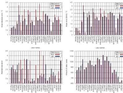
Measured and modelled lake surface temperatures were com-pared for the full experiment period 2010–2014. The model values were sampled for the ice-free season at 08:00 local time to correspond to the measured values. Figure 11 shows

Figure 9.Locations of 27 lake verification sites (© Google Maps 2019).

Figure 10.Lake depths and their differences in metres for 27 verification sites; OBS – measured by SYKE, OPR – from the ECMWF operational file and NEW – from the upgraded file.

Table 3.Locations of 27 verification lake sites; lake morphological parameters measured by SYKE and from ECMWF Tco1279 fields.

No. Lake ID Lake name Coordinates, deg In situ depth, m In situ area, Modelled mean depth, m

Latitude Longitude Mean Maximum km2 Operational New

1 44111001 Pielinen 63.2705 29.6067 10.1 61.0 894.2 5.0 10.0

2 42721001 Kallavesi 62.7616 27.7826 9.7 75.0 316.1 17.0 7.0

3 42111001 Haukivesi 62.1083 28.3887 9.1 55.0 560.4 2.0 7.0

4 41121001 Saimaa 61.3377 28.1158 10.8 85.8 1377.0 2.0 18.0

5 146311001 Paajarvi1 62.8638 24.7894 3.8 14.9 29.5 25.0 2.9

6 147311001 Nilakka 63.1146 26.5268 4.9 21.7 169.0 17.0 7.0

7 147111001 Konnevesi 62.6326 26.6046 10.6 57.1 189.2 25.0 7.0

8 148211001 Jaasjarvi 61.6310 26.1351 4.6 28.2 81.1 25.0 6.1

9 142211001 Paijanne 61.6139 25.4820 14.1 86.0 864.9 13.0 13.9

10 141711001 Ala-Rievel 61.3035 26.1718 11.2 46.9 13.0 25.0 7.0

11 149321001 Kyyvesi 61.9988 27.0796 4.4 35.3 130.0 25.0 5.0

12 210821001 Tuusulanja 60.4414 25.0544 3.2 9.8 5.9 3.0 6.2

13 340311001 Pyhajarvi 61.0011 22.2913 5.5 26.2 155.2 4.5 5.0

14 357211001 Langelmave 61.5353 24.3705 6.8 59.3 133.0 25.0 7.0

15 358331003 Paajarvi2 61.0635 25.1325 14.8 85.0 13.4 13.2 12.9

16 354121001 Vaskivesi 62.1416 23.7635 7.0 62.0 46.1 28.0 7.0

17 359311007 Kuivajarvi 60.7855 23.8596 2.2 9.9 8.2 9.0 7.0

18 353111001 Nasijarvi 61.6318 23.7505 14.7 65.6 210.6 28.0 7.0

19 470311001 Lappajarvi 63.1480 23.6706 6.9 36.0 145.5 2.0 18.0

20 595411001 Pesiojarvi 64.9451 28.6502 3.9 15.8 12.7 7.0 6.6

21 598111001 Rehja-Nuas 64.1840 28.0162 8.5 42.0 96.4 8.0 10.0

22 593111001 Oulujarvi 64.4500 26.9700 7.0 35.0 887.1 2.0 7.0

23 656321001 Ounasjarvi 68.3771 23.6016 6.6 31.0 6.9 3.0 7.0

24 655921001 Unari 67.1725 25.7112 7.0 24.8 29.1 2.0 7.0

25 676401001 Kilpisjarv 69.0070 20.8160 19.5 57.0 37.3 18.0 17.8

26 680721002 Kevojarvi 69.7515 27.0148 11.1 35.0 1.0 14.0 7.0

27 711111001 Inarijarvi 69.0821 27.9245 14.3 92.0 1039.4 14.0 14.0

Model errors may be different during different seasons de-pending on the model physics. It was shown that FLake has the best performance in the boreal zone during autumn, when lakes are mixed (Choulga and Kourzeneva, 2014), provided that the lake depth is correct. Thus, it is interesting to dig into details and to verify the model results for different seasons, depending on lake mixing regime. Typically, lakes in the

bo-real zone are dimictic (Lewis, 1983) and have five main sea-sons in relation to the mixing and ice cover:

i. spring mixing, when lakes are mixed till the bottom and the mixed layer depth equals the lake depth,

Figure 11.MAE, bias, SD and amount of data calculated over the total period of 2010–2014 for 27 verification sites; GTZP (red) – experiment with operational Dwater, GTZL (blue) – with upgraded Dwater.

iii. autumn mixing period, which is usually longer than the spring one,

iv. winter lake cooling period with the inverse temperature stratification, between the temperature of maximal den-sity and start of ice formation, and

v. winter, when lakes are covered with ice.

However, this classical pattern is approximate: it may be dis-torted, depending on the lake depth and the atmospheric forc-ing. For example, a stratified summer period may be inter-rupted by a short mixing period. Also, in early spring the in-verse temperature stratification may appear. Patterns of mix-ing and ice periods may be defined from the modellmix-ing re-sults. Figure 12 shows ice-covered (blue), mixed (red) and stratified (green) periods, defined for different lakes for the model experiments GTZPOPR and GTZLNEW. Most of the selected lakes show rather complex behaviour with a dis-torted classical pattern. For example, lakes Paajarvi2 and Kuivajarvi may have multiple ice and mixing periods dur-ing the year. Some lakes change patterns from one experi-ment to another, because of noticeable depth changes (e.g. lakes Haukivesi and Saimaa). To ease the verification pro-cess, these patterns were smoothed to better correspond to the dimictic lake classical pattern (simplified by merging the

short period of the inverse temperature stratification with au-tumn mixing). For each lake in both experiments, each year was separated into four main uninterrupted lake seasons, ac-cording to the modelling results. Figure 13 shows the results: i. winter period (blue), which contains the merged ice pe-riods when the ice-free time between them is 30 d or less;

ii. spring and autumn mixing periods (red and yellow re-spectively), which contain the merged mixed periods (when the mixed layer depth is approximately equal to the lake depth, with the maximum difference of 10 cm allowed) when the stratified regime between them is 20 d or less; and

iii. the stratified summer period (green), which is defined as a residual between spring and autumn periods.

Figure 12.Lake seasons for 2010–2014 for 27 verification sites based on operational(b)and upgraded(a)Dwater; blue – lake is ice-covered, red – lake is mixed till the bottom, green – lake is stratified (ice-free and non-mixed, residual period).

Distribution of model errors in terms of TML depend-ing on a mixdepend-ing season is shown in Figs. 14–17. The im-portant note is that bias in both experiments in all seasons was predominantly cold (positive) and large. It was so large that SD was smaller than bias. In other FLake model error studies bias was dependent on the season. For example, in Kourzeneva (2014), where forcing was from the High Reso-lution Limited Area Model (HIRLAM) (Unden et. al, 2002), in summer for the same Finnish lakes there was a strong warm bias, while in spring bias was cold. Errors inTML simu-lations depend on FLake itself, on the errors in Dwater, which is the main lake model parameter, and on the errors in forc-ing. Since the results of current experiments differ from the other studies, it should be suggested that in present research errors came from the forcing – ERA5 is supposedly too cold

Figure 13. Uninterrupted lake seasons for 2010–2014 for 27 verification sites based on operational(b)and upgraded(a)Dwater; blue – winter, red – spring mixing, green – stratified summer, yellow – autumn mixing period.

may be reflected in SD scores because they relate to the di-urnal cycle amplitude in the present experiments. These sug-gestions are in accordance with the obtained results. For all lakes, where upgraded Dwater was smaller than the opera-tional one, GTZLNEWbias was smaller in spring and larger in autumn compared with GTZPOPR (e.g. lakes Konnevesi and Vaskivesi). And vice versa, for all lakes, where upgraded Dwater was larger than the operational one, GTZLNEW bias was larger in spring and smaller in autumn compared with GTZPOPR(e.g. lakes Haukivesi and Oulujarvi). This was in-dependent of whether new Dwater is closer to the reality or not. For example, for lakes Lappajarvi and Saimaa, where upgraded Dwaterbecame larger and even further from the re-ality than operational, GTZLNEWautumn bias improved, due to compensating errors (good result for the wrong reason).

The only exception was Lake Niilakka, whose autumn bias was negative (warm). For the combined spring–autumn mix-ing period, bias scores were generally better, or the effect was neutral. For the summer stratified period, the impact of Dwater on the bias scores was neutral or slightly positive. The SD scores were best for the autumn mixing period, when the lake surface temperature diurnal cycle is absent. For lakes Saimaa and Lappajarvi, the summer period SD scores were worse in GTZLNEW compared with GTZPOPR; however, Dwater was worse as well. For the lakes with better Dwater values in GTZLNEW, SD scores improved or remained unchanged for all seasons. The exception was Lake Oulujarvi: its SD scores deteriorated, mainly in autumn.

Figure 14.MAE, BIAS, SD and amount of data calculated over all mixing periods 2010–2014 for 27 verification sites; GTZP (red) – experiment with operational Dwater; GTZL (blue) – with upgraded Dwater.

Figure 16.Same as Fig. 14 but calculated over all autumn mixing periods.

Table 4.Ice formation/disappearance dates for 2010–2014 of 27 verification sites; OBS – measured by SYKE; GTZP_OPRand GTZLNEW– ECMWF experiments with operational and updated Dwaterrespectively; improvements in the freeze-up date in GTZLNEWcompared with GTZPOPRare marked in bold and degradation in italics (only cases when the difference was larger than 14 d).

No. Lake name Year 2010 2011 2012 2013 2014 2010 2011 2012 2013 2014

Data Ice melting Ice freezing

1 Pielinen OBS 05/10 05/02 05/14 05/08 04/28 11/22 12/12 12/03 12/02 12/18 GTZPOPR 05/23 05/26 05/21 05/24 05/17 11/11 11/21 11/10 11/25 11/08 GTZLNEW 05/23 05/26 05/21 05/24 05/17 11/15 11/30 11/15 11/27 11/14

2 Kallavesi OBS 05/08 05/06 05/08 05/06 04/19 11/29 99/99 01/01 12/09 12/24 GTZPOPR 05/22 05/28 05/20 05/23 05/16 11/27 12/30 12/03 12/09 12/18 GTZLNEW 05/22 05/26 05/21 05/24 05/18 11/15 11/30 11/30 11/30 11/22

3 Haukivesi OBS 05/04 05/08 05/07 05/05 04/19 11/27 99/99 01/02 12/10 12/22

GTZPOPR 05/21 05/25 05/18 05/21 05/13 11/08 11/18 10/29 11/24 10/23 GTZLNEW 05/22 05/24 05/18 05/22 05/13 11/20 11/30 11/30 11/30 11/22 4 Saimaa OBS 05/02 04/27 05/02 05/06 04/17 11/25 12/25 12/05 11/23 12/22

GTZPOPR 05/15 05/18 05/11 05/15 04/28 11/18 11/21 10/31 11/26 10/23 GTZLNEW 05/15 05/16 05/11 05/17 04/30 11/28 01/04 12/05 12/15 12/23 5 Paajarvi1 OBS 05/02 04/27 05/03 05/02 04/18 11/20 12/12 11/30 11/29 12/05 GTZPOPR 05/14 05/10 05/06 05/05 04/15 11/21 12/28 12/02 12/03 12/15 GTZLNEW 05/13 05/10 05/06 05/05 04/15 10/16 11/16 10/27 10/20 10/22

6 Nilakka OBS 05/05 05/02 05/08 05/06 04/23 11/17 12/12 11/29 11/23 12/02 GTZPOPR 05/23 05/28 05/25 05/24 05/18 11/27 12/29 12/03 12/05 12/18 GTZLNEW 05/23 05/26 05/25 05/24 05/17 11/12 11/30 11/17 11/26 11/20

7 Konnevesi OBS 05/05 05/02 05/05 05/05 04/20 11/22 12/31 12/02 99/99 01/12 GTZP_OPR 05/08 05/09 05/03 05/04 04/14 11/22 01/01 12/03 12/08 12/22 GTZLNEW 05/08 05/09 05/03 05/04 04/14 11/11 11/30 11/10 11/26 10/24

8 Jaasjarvi OBS 04/27 04/27 05/01 05/02 04/11 11/21 99/99 01/01 12/05 12/19 GTZPOPR 05/02 05/04 04/29 04/30 04/13 11/25 01/07 12/04 12/10 12/24 GTZLNEW 05/02 05/04 04/29 05/01 04/13 11/18 12/08 11/30 11/27 10/24

9 Paijanne OBS 05/04 04/30 05/01 05/03 04/12 11/27 99/99 01/01 12/15 12/26 GTZPOPR 05/19 05/23 05/15 05/19 05/06 11/26 12/31 12/03 12/08 12/18 GTZLNEW 05/19 05/23 05/17 05/19 05/05 11/27 12/31 12/03 12/10 12/19

10 Ala-Rievel OBS 04/28 05/01 05/02 05/01 04/13 11/23 99/99 01/01 12/08 12/24 GTZPOPR 05/02 05/03 04/28 05/01 04/13 11/26 01/08 12/04 12/10 12/23 GTZLNEW 05/02 05/04 04/28 05/01 04/13 11/19 12/10 11/30 11/30 11/23

11 Kyyvesi OBS 99/99 04/30 99/99 05/02 04/12 11/21 99/99 12/03 11/30 12/22 GTZPOPR 05/09 05/11 05/05 05/05 04/15 11/25 01/03 12/04 12/10 12/19 GTZLNEW 05/10 05/11 05/05 05/06 04/15 11/10 11/21 11/09 11/26 10/23 12 Tuusulanja OBS 04/21 04/25 04/24 04/29 04/05 11/09 11/21 11/10 11/25 12/01

GTZP_OPR 04/25 04/27 04/20 04/26 03/25 11/19 12/09 10/28 11/26 10/23

GTZLNEW 04/25 04/27 04/20 04/26 03/23 11/20 01/02 12/01 11/30 12/02 13 Pyhajarvi OBS 04/26 05/02 04/26 05/01 04/03 11/22 99/99 01/07 12/11 12/24

Table 4.Continued.

No. Lake name Year 2010 2011 2012 2013 2014 2010 2011 2012 2013 2014

Data Ice melting Ice freezing

15 Paajarvi2 OBS 99/99 99/99 99/99 99/99 99/99 99/99 99/99 99/99 99/99 99/99 GTZPOPR 05/01 05/02 04/27 04/30 04/12 11/22 01/02 12/01 12/02 12/21 GTZLNEW 05/01 05/02 04/27 04/30 04/12 11/22 01/02 12/01 12/02 12/19

16 Vaskivesi OBS 04/27 04/28 04/30 05/01 04/12 11/23 12/31 12/02 12/08 11/30

GTZPOPR 05/06 05/06 04/30 05/02 04/13 11/23 01/07 12/04 12/10 12/22 GTZLNEW 05/05 05/08 04/30 05/03 04/13 11/13 12/07 11/10 11/26 11/22 17 Kuivajarvi OBS 04/21 04/26 04/24 04/29 04/02 11/22 99/99 01/01 12/01 12/22 GTZPOPR 05/01 05/05 04/26 05/01 04/09 11/21 01/01 12/01 12/01 12/21 GTZLNEW 05/01 05/06 04/26 05/01 04/09 11/20 12/12 12/01 11/30 12/04

18 Nasijarvi OBS 04/29 05/01 05/01 05/03 04/13 11/29 99/99 01/10 99/99 01/14 GTZPOPR 05/07 05/10 04/29 05/04 04/13 11/28 01/10 12/08 01/14 12/26 GTZLNEW 05/07 05/11 05/01 05/05 04/13 11/19 12/12 12/01 11/30 12/04

19 Lappajarvi OBS 05/04 05/03 05/02 05/03 04/17 11/22 12/31 12/03 11/22 12/22

GTZPOPR 05/16 05/13 05/09 05/09 04/18 10/17 11/16 10/27 10/19 10/22 GTZLNEW 05/16 05/13 05/09 05/09 04/17 11/21 12/28 12/02 11/30 12/14 20 Pesiojarvi OBS 99/99 99/99 99/99 99/99 99/99 99/99 99/99 99/99 99/99 99/99 GTZP_OPR 05/18 05/17 05/16 05/14 05/11 10/28 11/16 10/27 10/20 10/18 GTZLNEW 05/18 05/17 05/16 05/14 05/11 10/27 11/16 10/26 10/20 10/18

21 Rehja-Nuas OBS 05/04 05/02 05/01 05/04 04/20 11/14 99/99 11/09 11/27 11/07 GTZPOPR 05/17 05/16 05/14 05/11 04/29 11/09 11/20 10/30 11/21 10/22 GTZLNEW 05/17 05/16 05/14 05/11 04/28 11/10 11/21 11/08 11/22 10/23

22 Oulujarvi OBS 05/15 05/10 05/13 05/14 05/02 11/24 99/99 99/99 12/04 12/18

GTZPOPR 05/25 05/28 05/25 05/27 05/20 10/27 11/15 10/27 10/20 10/18 GTZLNEW 05/25 05/28 05/25 05/27 05/20 11/11 11/21 11/10 11/15 11/08 23 Ounasjarvi OBS 05/24 05/23 05/27 05/25 06/01 11/06 11/16 10/28 11/12 10/31 GTZPOPR 06/03 06/02 05/31 05/30 06/05 10/15 10/14 10/18 10/16 10/13 GTZLNEW 06/03 06/02 05/31 05/30 06/05 10/25 11/11 10/21 10/19 10/17 24 Unari OBS 05/19 05/15 05/21 05/18 05/23 11/06 11/19 10/26 11/08 11/02

GTZPOPR 06/02 05/30 05/28 05/26 05/29 10/15 10/15 10/18 10/16 10/13 GTZLNEW 06/02 05/30 05/28 05/26 05/28 10/30 11/15 10/23 10/20 10/17 25 Kilpisjarv OBS 06/15 06/09 06/19 06/03 06/19 11/10 12/07 11/14 11/19 11/05 GTZP_OPR 06/24 06/13 06/24 06/05 06/24 10/25 11/10 10/23 10/21 10/22 GTZLNEW 06/24 06/13 06/21 06/05 06/24 10/25 11/10 10/23 10/21 10/22

26 Kevojarvi OBS 05/23 05/25 05/26 05/19 05/27 10/29 11/18 10/27 11/07 10/25 GTZPOPR 06/07 06/07 06/01 06/01 06/08 10/30 11/16 10/28 10/23 10/19 GTZLNEW 06/07 06/07 06/01 06/01 06/08 10/26 11/04 10/23 10/18 10/17

27 Inarijarvi OBS 06/03 06/03 05/31 05/25 06/02 11/26 99/99 11/26 11/27 11/13 GTZPOPR 06/09 06/08 06/05 06/02 06/07 11/07 11/21 11/10 11/09 11/02 GTZLNEW 06/09 06/08 06/05 06/02 06/07 11/07 11/21 11/10 11/09 11/02

formation/disappearance dates from the SYKE in situ archive and based on experiment results with operational (GTZPOPR) and upgraded (GTZLNEW) Dwater for 27 lake sites. In gen-eral, present experiments showed too late ice melt in spring and too early ice formation in autumn; this is in accordance with suggestion of a cold bias in forcing. Thus, compensation

exper-Table 5.Locations of in situ water surface temperature and ice formation/disappearance measurement points and distance between them for 27 verification sites; latitude and longitude in degrees, distance in kilometres.

Lake name Measurement location (ML) coordinates, deg Distance

Water surface temperature (WST) Ice between WST

Latitude Longitude Note Latitude Longitude Note and ice ML, km

Pielinen 63.2705 29.6067 middle of the lake 63.5418 29.1314 on/close to the lake shore 38.45 Kallavesi 62.7616 27.7826 middle of the lake 62.8993 27.7317 on/close to the lake shore 15.56 Haukivesi 62.1083 28.3887 middle of the lake 62.1107 28.6064 on/close to the lake shore 11.37 Saimaa 61.3377 28.1158 middle of the lake 61.5008 27.2636 on/close to the lake shore 49.00 Paajarvi1 62.8638 24.7894 middle of the lake 62.8474 24.8142 close to the lake shore 2.22 Nilakka 63.1146 26.5268 middle of the lake 63.1993 26.6696 on/close to the lake shore 11.87 Konnevesi 62.6326 26.6046 middle of the lake 62.6166 26.3492 on/close to the lake shore 13.23 Jaasjarvi 61.6310 26.1351 middle of the lake 61.5674 26.0467 on/close to the lake shore 8.50 Paijanne 61.6139 25.4820 middle of the lake 61.1760 25.5362 on/close to the lake shore 48.88 Ala-Rievel 61.3035 26.1718 middle of the lake 61.3358 26.2012 on/close to the lake shore 3.93 Kyyvesi 61.9988 27.0796 middle of the lake 62.0127 27.1895 on/close to the lake shore 5.96 Tuusulanja 60.4414 25.0544 middle of the lake 60.4168 25.0427 on/close to the lake shore 2.82 Pyhajarvi 61.0011 22.2913 middle of the lake 61.1015 22.1802 on/close to the lake shore 12.70 Langelmave 61.5353 24.3705 middle of the lake 61.4180 24.1474 on/close to the lake shore 17.67 Paajarvi2 61.0635 25.1325 middle of the lake no station

Vaskivesi 62.1416 23.7635 middle of the lake 62.1175 23.9249 on/close to the lake shore 8.84 Kuivajarvi 60.7855 23.8596 middle of the lake 60.7821 23.8383 on/close to the lake shore 1.22 Nasijarvi 61.6318 23.7505 middle of the lake 61.5086 23.7725 on/close to the lake shore 13.78 Lappajarvi 63.1480 23.6706 middle of the lake 63.2595 23.6353 on/close to the lake shore 12.55 Pesiojarvi 64.9451 28.6502 middle of the lake no station

Rehja-Nuas 64.1840 28.0162 middle of the lake 64.1616 28.2441 on/close to the lake shore 11.36 Oulujarvi 64.4500 26.9700 middle of the lake 64.5509 26.8240 on/close to the lake shore 13.26 Ounasjarvi 68.3771 23.6016 close to lake shore 68.3975 23.7170 on/close to the lake shore 5.26 Unari 67.1725 25.7112 middle of the lake 67.1366 25.7416 on/close to the lake shore 4.22 Kilpisjarv 69.0070 20.8160 middle of the lake 69.0497 20.7881 on/close to the lake shore 4.90 Kevojarvi 69.7515 27.0148 middle of the lake 69.7566 27.0031 on/close to the lake shore 0.72 Inarijarvi 69.0821 27.9245 middle of the lake 68.9577 27.6942 middle of the lake 16.65

iments, but in freeze-up dates the difference was substantial. Errors were large – the ice melt date maximum error was 26 d (lake Niilakka in 2011) and ice freeze-up date maximum er-ror was 61 d (lake Oulujari in 2017, GTZPOPR). The ice-off date errors were not dependent on Dwater; the largest errors corresponded to large-area lakes (e.g. lakes Haukivesi and Kallavesi; see Table 4). It can be explained by the fact that the ice formation/disappearance in situ measurements rep-resent the freeze-up and break-up dates in the visible area around the observer’s location (usually on the shore), and due to physiographic features (e.g. complicated rugged coast) and/or meteorological conditions (e.g. low clouds, rain) can be not fully representative for the whole 9 by 9 km grid box. Ice measurement locations differ from temperature measure-ment locations, and the distance between these two can vary from 0.7 to 49.0 km; see Table 5. SYKE also provides the break-up dates in far central parts of the lake and perma-nent freeze-up dates of the visible area around the observer’s location, but the amount of data is very limited and can-not be used for verification. However, it gives a hint that

freeze-up dates improved for wrong reasons). If during the freeze-upgrade Dwaterdecreased, errors became larger (e.g. lakes Konnevesi and Vaskivesi). This agrees with the autumnTMLbias scores: if they improve, the freeze-up dates improve as well. 4.3 Discussion

Upgraded lake-related fields were tested for 5 successive years to capture short climate deviations (one particular year can be slightly warmer or colder than the average one) yet not to deal with major water distribution and/or inland wa-ter body depth changes that can occur in a 10-year period and that would have to be taken into account when compared against in situ measurements. Current verification included only 27 lake sites over Finland which are freely available online; it would be useful to compare model results with measurements from the other countries and climate zones as the IFS is a global forecasting system. For that, data from remote sensing could be beneficial, although they con-tain gaps and cloud contamination problems. Experiments run with model cycle CY43R3. New cloud physics in the model cycle’s recent upgrade led to improvements in calcu-lating 2 m temperature and humidity and precipitations (es-pecially near coasts), which can lead to better agreement of the modelled and in situ lake surface temperature and ice for-mation/disappearance dates respectively. Verification of op-erational and upgraded Dwater for 27 Finnish lakes resulted in significant reduction of errors, though it is still possible to upgrade Dwater with new measurements and test new ag-gregating techniques in order to better represent initial high-resolution lake depth fields. Verification in terms of modelled and in situ lake surface temperature for the whole 5-year pe-riod showed general error reduction for 12 %–14 %. Seasonal verification also showed an overall error reduction, although the amount of data during the 5-year period was not suffi-cient to always have statistically significant results. Seasonal verification also revealed the cold bias in the forcing and sit-uation, when changes in the Dwaterparameter compensate for this bias. For more detailed ice formation/disappearance date verification and explanation of the results, first and perma-nent ice formation/disappearance dates in a far central part of the lake (compatible with an IFS model high-resolution 9 km grid) are needed.

5 Conclusion

Earth system models used for weather and climate moni-toring and forecasting applications, including the IFS, need lower boundary conditions (skin temperature, surface fluxes of heat, moisture and momentum) to calculate the evolution of dynamic processes in the atmosphere and to produce a usable weather forecast. To compute them sufficiently ac-curately, an up-to-date ecosystem map is needed. Nowadays human activities influence Earth’s surface and adapt it to

so-cietal needs on relatively short timescales, for example to construct new artificial lakes to supply people and/or crops in arid places with water, or to create new islands to build homes. Inland water bodies can influence local climate by over 1 K (Balsamo et al., 2012), and the influence on lo-cal weather can be even more pronounced: correct lake sur-face state (ice/no ice) in winter conditions can lead to up to 10 K difference in 2 m temperature (Eerola et at., 2014). Ma-jor changes in water bodies can occur in just a few years, which means that ecosystem-based maps used for numer-ical weather prediction need to be updated regularly. The most frequent updates of ecosystem maps come from satel-lite products, which are becoming available at increasingly high resolution. The main obstacle to using these maps in the model without any modification is that they do not distin-guish between ocean and inland water. An automatic algo-rithm to separate ocean and inland water has been presented in this article. This new algorithm may be used by anyone in the environmental modelling community. This algorithm can also be used to distinguish between rivers and lakes, but it will require more testing and tuning of parameters before it can be applied globally. For the IFS, the most reliable data sources are used to ensure the best possible representation of the global inland water distribution. The continuous water depth field was updated with new ocean and lake bathyme-tries, new versions of the lake database, and indirect depth estimates based on the geological origin of lakes. Verification of the depth field for 27 Finnish lake sites showed significant lake depth error reductions in the GLDBv3 dataset compared to GLDBv1. Verification in terms of the lake water surface temperature showed an overall error reduction of between 12 % and 14 %. Seasonal lake water surface temperature ver-ification, according to lake mixing periods (spring mixing, summer stratification and autumn mixing), showed an over-all error reduction, although forcing in the numerical exper-iments was too cold, and it may be that this error was com-pensated for by lake depth parameter errors. Winter season verification based on an ice formation/disappearance date comparison was also influenced by the problem of overly cold forcing and compensating errors. A more detailed ice formation/disappearance date verification and further exper-iments are clearly needed. The first and permanent ice for-mation/disappearance dates in the far central part of the lake (compatible with an IFS model high-resolution 9 km grid) would be very helpful for verification. Lake depth and lake cover variability over time are recognised as key aspects for future developments. The present study aims to document the methodology and to provide experimental evidence of its benefits, and it will be used to characterise temporal varia-tions (e.g. in annual or monthly updates).