AN EFFICIENT LIVER SEGMENTATION USING KERNEL SPARSE
CODING AUTOMATED (KSCA) APPROACH
Rajesh Sharma R.1 and Marikkannu P.2
1Department of IT, Hindusthan College of Engineering and Technology, Coimbatore, Tamilnadu, India 2Department of IT, Anna University Regional Centre, Coimbatore, Coimbatore, Tamilnadu, India
E-Mail: [email protected]
ABSTRACT
Computed Tomography (CT) images have been widely used for diagnosis of liver disease and volume measurement for liver surgery or transplantation. The approach is presented with respect to liver segmentation, but it can be easily extended to any other soft tissue by setting appropriately the values of the parameters for the splitting and merging algorithm and for the region growing refinement step. Sparse coding with data-adapted dictionaries has been successfully employed in several image recovery and vision problems. A novel, automated segmentation technique for detecting affected region in liver was proposed in this paper. In the new approach, we constructed ensemble kernel matrices using the pixel intensities and their spatial locations, and obtained kernel dictionaries for sparse coding pixels in a non-linear feature space. The resulting sparse codes were used to train an Extreme Learning Machine (ELM) classifier that determines if a pixel in the image belongs to an affected region. From the experimental results using ten test datasets distributed for the competition, it was confirmed that our method kernel sparse coding based liver segmentation performs better than previous methods or models.
Keywords: liver disease, segmentation, auto-context model (ACM), kernel sparse coding automated approach, ELM.
INTRODUCTION
In recent years, medical image segmentation has become an active area of research and it attracts more and more researchers for novel innovations. Image segmentation automatically explores the internal structures of the patient, which may be anatomical (organs) and pathological (lesions). Automatic segmentation of lesions in a large image database has attracted the attention of several researchers as it assists in diagnosis [1], by identifying possibly forgotten lesions, and also to speed up the process of analysis. Liver is one of the most important organs of the human body. When it is affected by a tumoral pathology, it is possible to operate it by cutting the damaged portion. But the segmentation has to be done with the rules of volumetric and very specific vascularization. The medical imaging is then used to detect and visualize the internal structures. These structures do not appear in a single image, but need several acquisitions which will therefore be compared. The tumoral or hepatic volumetric is possible only after a period of segmentation of these images. Liver analysis plays a vital role in the therapeutic strategy for hepatic diseases. Therefore, the automatic segmentation of the liver has influenced a number of researchers with its importance and it assists in diagnosis of liver diseases such as steatosis, fibrosis, etc. Segmentation of a liver from a three dimensional CT volume serves as the initial process in image-based hepatic investigations [2, 3]. Even though a number of techniques have been developed and available in the literature, fully automatic liver segmentation from a 3D volume is still a challenging factor due to the large variations in liver shapes and in the intensity pattern inside and along liver boundaries.
The main aim of the present research work is to develop a novel approach for automatic liver segmentation
to obtain its internal structures and tumors in a more efficient manner. Auto-Context Model (ACM) has been used in the automatic liver segmentation approach. The present research work extends the approach of HongweiJi in [14] which used the ACM model for segmentation. The present research work uses kernel Sparse Coding Automated approach for liver segmentation which overcomes the limitations in ACM approach.
PREVIOUS WORKS
Max-Flow/Min-Cut method [4] this approach is a semi-automatic segmentation of the liver depending on graph theory and more particularly on the "Graph Cuts". In this scenario, the issue of segmentation is regarded the separation of an image into two classes "object" and "bottom". This approach for semi-automatic segmentation integrates some of the voxels of the volume to one of these two classes. This initial association acts then as base of training for the ultimate segmentation of the volume. This technique implements an energy minimization approach based on partitioning a graph into two sub-graphs by cutting minimum capacity.
Bae et al. [5] used simple thresholding and logic
Shimizu et al. [6] used the equivalent CT values from four different input images of the same liver to attain the rough contour. The main limitation of this approach is that four complete datasets are needed for effective segmentation of one liver. This needs four different CT scans of the same patient in succession, and computationally it requires four times the memory and processing power that is used when analyzing a single dataset. Computer-Aided Diagnosis (CAD) is being widely used to improve the interpretation components of medical imaging [7, 8]. Moreover, Computer-Aided Surgery (CAS) is carried out on computerized surgical planning and image-guided surgery by examining the Region-Of-Interest (ROI) in the medical image. Volume measurement is also of major significance in different fields of medical imaging where doctors need some assessments for surgical decisions.
Seoa multi-stage automatic hepatic tumor segmentation approach is presented [9]. It initially segments the liver, and eliminates hepatic vessels from the liver. Then, a hepatic tumor is segmented through the optimal threshold value with minimum total probability error. Active contour algorithm has been widely used in tumor segmentation. Yim et al. used watershed and active contour algorithms for volumetric investigation on ten hepatic metastatic lesions in 36 CT slices [10]. Lu et al. also used the active contour with aspecific initial contour to attain the tumor boundary [11]. Zhao et al. developed a region growing algorithm through intensity distributions of the seed ROI offered by users to delineate liver metastases. Particular shape constraints have been used to prevent the region growing from leaking into surrounding tissues [12]. But, there are certain drawbacks in the above said existing techniques. Most of the above said approaches segment the tumor in 2D. When considering CT volumetric data, segmentation is carried out slice by slice, and then the 2D results are integrated into a volume. Moreover, these techniques were tested on different data sets and evaluated using different standards. Hence it is difficult to compare their performance. To benchmark 3D liver tumor segmentation methods, the organizer of “3D Liver Tumor Segmentation Challenge 2008”[13] provided CT scans of livers from four patients with ten lesions manual segmented as training data, together with other six CT scans of livers with ten lesions (not segmented) as the testing data.
Figure-1. Segmentation of results.
Figure-1 Shows the segmentation process of the liver image. That perform the process of marked the region, then enhance the image after the do the segmentation process.
Hongwei et al. [14] presented an Auto-context Model (ACM) based automatic liver segmentation algorithm, which integrates ACM, multi-atlases and mean-shift techniques to segment liver from 3D CT images. This algorithm is learning based approach and can be categorized into two stages. At the initial training stage, ACM learns a series of classifiers in each atlas space. Through multiple atlases, multiple sequences of ACM-based classifiers are attained. In the second segmentation stage, the test image will be segmented in each atlas space through each sequence of ACM-based classifiers. The ultimate segmentation result will be attained by fusing segmentation results from all atlas spaces through a multi-classifier fusion approach. Even though ACM based liver segmentation is effective, it has some limitations:
The features on the context information are still somewhat limited.
Different auto-context models require to be trained for different applications.
The algorithm is a supervised approach and thus needs a set of well-annotated ground truth data, which might not always be available or can be difficult to obtain.
Method is a supervised learning technique, it needs a set of manual reference segmentations (ground-truth data), which is sometimes difficult to obtain.
The limitation of Mean-shift method is that, it is a time consuming image segmentation algorithm. In order to overcome these problems, kernel sparse coding segmentation algorithm is used for liver segmentation in the present research work.
METHODOLOGY
The main contribution of the present research work is threefold. Initially, the pre processing is done followed by segmentation and classification. In segmentation we use kernel sparse coding for liver segmentation initially, dictionary design through kernel similarities, representation of test samples and finally discrimination of resultant codes.
noise, image contrast and improves the boundaries of the liver. It is used for separating the liver image from adjacent organs by improving the boundaries. The second step of the proposed preprocessing technique is applying the laplacian filtering technique and it is mainly focused on the image intensity changes and used for improving the edges of the liver. In this paper it is combined with the stick filter for best results and the kernel of the Laplacian filter can be calculated as given equation.
(I)
Sparse Coding and Dictionary Learning Sparse models have been widely used in image analysis as several naturally occurring images can be efficiently formulated as a sparse linear combination of elementary features [15]. The elementary features are normalized to unit norm and stacked together to form the dictionary matrix. Given a sample y , and a dictionary the generative model for sparse coding is given as , where is the sparse code with a small number of non-zero coefficients and n is the noise component [16]. The sparse code can be computed by solving the convex problem
(1)
Where indicates the norm, and is a convex surrogate for the norm which counts the number of non-zero elements in a vector [17]. Some of the approaches used to solve (1) include the basis pursuit [18]; feature-sign search [19] and the least angle regression algorithm with the LASSO modification (LARS-LASSO) [20]. When presented with a adequately large set of training data samples, , the dictionary can be learned, and the corresponding sparse codes can be obtained by solving equation (2).
(2)
Where and denotes the Frobenius norm of the matrix. Equation (2) can be solved as an alternating minimization problem, where the dictionary is learned by fixing the sparse codes, and the sparse codes are obtained by fixing the dictionary. Dictionaries fixed to the data provide superior performance when compared to predefined dictionaries in a number of applications [21, 14]. Moreover, being valuable in data representation issues, there has been a recent surge of interest in using sparse models in several supervised, semi-supervised and unsupervised learning tasks such as clustering [22] and classification [23].
Kernel Sparse Coding for Liver Segmentation Sparse coding algorithms are mostly used for vectorized patches or feature vectors extracted from the images, through an over complete dictionary. It is typical in
machine learning techniques to utilize the kernel function to learn linear models in a feature space that captures the linear similarities. Kernel functions map the non-linear separable features into a feature space using a transformation in which similar features are grouped together. By carrying out sparse coding in the feature space , highly discriminative codes can be obtained for samples from different classes [16, 24, and 25].
Kernel Sparse Coding with the feature mapping function the generative model in F for kernel
sparse coding is given by . The data
sample y in the feature space is represented as and
the dictionary by the
kernel similarities and
can be calculated through pre-defined kernel functions. All further computations in the feature space will be carried out exclusively using kernel similarities. The problem of sparse coding in (1) can be posed in the feature space as
(3)
Expanding the objective in (3), the following equation is obtained
(4)
denotes the element vector
containing the elements matrix
containing the kernel similarities between the dictionary atoms. The kernel sparse coding problem can be efficiently solved through the feature-sign search algorithm. However, it is essential that the computation of kernel matrices incurs additional complexity. As the dictionary is fixed in (4), denotes computed only once and the complexity of computing alters as
significant performance. The clustering problem can therefore be posed as
(5)
Each dictionary atom is equivalent to a cluster center and each coefficient vector encodes the cluster association and the weight corresponding to the pixel. The alternating optimization for solving equation (5) consists of two steps: (a) cluster assignment, which involves finding the association and weight of each training vector and hence updating the sets and (b) cluster update, which involves updating the cluster center by finding the centroid of training vectors corresponding to each set .
In the cluster assignment step, the correlations of a training sample with the dictionary atoms can be
formulated as . If the dictionary
atom results in maximum absolute correlation, the index i is placed in set , and the corresponding non-zero coefficient is the correlation value itself. For the cluster let be the set of member vectors and be the row of corresponding non-zero weights. The cluster update involves solving the equation (6).
(6)
Denoting the singular value decomposition of
(7)
Rank-1 approximation, which also results in the optimal solution for equation (6), is given by
(8)
Where is the largest singular value, and and are the columns of and equivalent to that singular value. Equation (8) implies that and Let the Eigen decomposition of be and hence assuming the Eigen values are in descending order. From equation (7), Substituting for
and , is obtained which
results in
(9)
Note that ak completely defines dk. The cluster assignment and update steps arerepeated until convergence, i.e., when {Ck} K,k=1 does not change over iterations.
Representation Kernel sparse coding is used as an alternative to techniques such as kernel PCA for efficient data representation. Though, entire reconstruction of the
fundamental data from the kernel sparse codes need computation of pre-images [28], novel test samples can also be well approximated using the learned kernel dictionaries.
Discrimination Kernel sparse coding is well suited for supervised learning tasks. As the non-linear similarities between the training samples are taken into consideration while learning the dictionary, the resulting codes are highly discriminative. The kernel sparse codes are obtained for all the samples and the normalized cross correlation are computed between the sparse features. As kernel sparse codes promote discrimination, features belonging to a class are expected to be highly similar when compared with the samples from other classes.
PROPOSED ALGORITHM
The proposed algorithm is used for liver segmentation using Kernel Sparse Coding-Based Automated (KSCA) segmentation algorithm. In the algorithm the training set of images are taken which is used for aligning and segmentation purpose although the segmentation is unendorsed learning here we consider it as proven.The Kernel Matrix is generated through pixel intensities and spatial locations and the kernel dictionaries are attained based on kernel dictionary optimization and kernel sparse coding for sparse coding pixels in nonlinear feature space. The images are partitioned into K subsets by using K-line clustering algorithm along with the help of kernel sparse dictionary learning. The output of the clustering procedure sparse code trains the ELM classifier which is used to find the affected regions of the liver based on the pixel.
Combining Multiple Features When compared to using a single feature, using multiple features to characterize images has been a very successful approach for classification tasks. Though this method provides the flexibility of choosing features to describe different aspects of the underlying data, the result and illustrations are high-dimensional and the descriptors could be varied diversely. Therefore, there is a need to transform the features to a unified space that allows the recognition functions, and generate low dimensional compact representations for the images in the unified space. A set of R diverse descriptors are extracted from a given image. As the kernel similarities can be utilized to fuse the multiple descriptors, the base kernel matrix is constructed for each descriptor. A suitable distance function is given which evaluates the distance between two samples for the feature the kernel matrix can be constructed as
(10)
Where is a positive constant? Given the R base kernel matrices, , we can construct the ensemble kernel matrix as
A constructive alternate technique to fuse the descriptors is to attain the ensemble kernel matrix as
(12)
Where ⊙ denotes the Hadamard product between two matrices. Sparse codes calculated with the ensemble kernel matrices will take all the R features into consideration. Note that when combining kernel matrices, we need to ensure that the resulting kernel matrix also satisfies the Mercer’s conditions.
Figure-2. The figure depicts the proposed algorithm for automated liver segmentation.
Figure-2 Shows For a set of training samples, the ensemble kernel dictionary is obtained using Kernel K-lines clustering procedure and ELM classifier is used to classify the pixels.4.2. Algorithm
The proposed algorithm of this research work is Kernel Sparse Coding-based Automated (KSCA) segmentation algorithm. The kernel matrix is computed using RBF kernel on pixel intensity values for the subset of pixels T. in order obtain the ensemble kernel matrix, the fusion of intensity and spatial location matrix is take place.
(13)
The sparse codes attained with a dictionary learned in the ensemble feature space model the similarities of pixels according to both intensity and location of pixels. A group of training images, with active tumor regions, are utilized to learn a kernel dictionary with the kernel K-lines clustering process. Using the kernel sparse codes belonging to affected and non-affected regions, ELM classifier is used to classify the affected regions based on the pixel. For a test image, the required ensemble kernel matrices are obtained and the kernel sparse codes using the learned dictionary are computed.
ELM Description
ELM is a unified Single hidden Layer Feed forward Neural network (SLFN) with randomly generated
hidden nodes independent of the training data [29, 30]. For
N arbitrary distinct samples and (n is the number of dimensions of
input x, m is the number of classes of data). So a given set
of training samples the output of a
SLFN with L hidden nodes can be represented by
(14)
where and are the parameters of hidden node which could be randomly generated. is the output of the hidden node with respect to the input x. And bi is the weight connecting the hidden node to the output node. Equation (1) can be written compactly as
(15)
is the transpose of a matrix or vector . H is called the hidden layer output matrix of the network [30]; the column of H is the hidden node’s output vector with respect to inputs : and the row of is the output vector of the hidden layer with respect to input . It has been proved in theory [29, 30] that SLFNs with random hidden nodes have the universal approximation capability, and the hidden nodes can be randomly generated independent of the training data.
After the hidden nodes are randomly generated and given the training data, the hidden-layer output matrix H is known and need not be tuned. Thus, training SLFNs simply amounts to getting the solution of a linear system (2) of output weights according to Bartlett’s theory [30] for feed forward neural networks, in order to get the better generalization performance, ELM not only tries to reach the smallest training error but also the smallest norm of output weights.
And
Under the constraint of equation (5), a simple representation of the solution of the system (2) is given explicitly by Huang et al. [31] as
(16)
Where the Moore-Penrose is generalized inverse of the hidden-layer output matrix H. If the N training data are distinct, H is column full rank with high probability when . In real applications, the number of hidden nodes is always less than the number of training data . Thus
Huang et al. [31] have proved SLFNs with a wide type of random computational hidden nodes. Additive and RBF hidden nodes are used often in applications. For example, additive hidden node with the activation function
(e.g., sigmoid, threshold, sin/cos, etc.), is given by
Where alpha is the weight vector connecting the input layer to the hidden node and is the bias of the hidden node. denotes the inner product of
vectors The three-step simple learning
algorithm can be summarized as follows:
Algorithm 1
Given a training set , the hidden-node output function and hidden-node number L: Step 1: Randomly assign hidden-node parameters
Step 2: Calculate the hidden-layer output matrix H; Step 3: Calculate the output weight vector
In this paper ELM is used as classifier to identify the pixels belonging to affected region of liver.
EXPERIMENTS
The results are compared to manual segmentations performed by a radio-oncology specialist, based on both the subjective visual quality and quantitative standards such as Accuracy (Acc) and Correspondence Ratio (CR). The learning-based liver segmentation technique is evaluated based on the training and testing datasets of MICCAI 2007 liver segmentation challenge (http://www.sliver07.org). There are 20 contrast-enhanced abdominal CT images in the training datasets and 10 in the testing datasets. All images have a spatial resolution of pixels in each transversal slice and the pixel spacing varies from 0.55 to 0.9mm. The inter-slice distance varies from 0.5 to 5mm. In this paper, 10 CT images from the training datasets (denoted as “TrainIM”) are randomly chosen for learning.
The remaining 10 CT images in the training datasets (represented as“TestIM1”) and 10 CT images in the testing datasets (represented as “TestIM2”) are used
for evaluation. The MICCAI 2007 workshop provides manual liver labels only for the training datasets, not for the testing datasets. Thus do “TestIM1” for quantitative evaluation and then both “TestIM1” and “TestIM2” for equality evaluation.
Figure-3. Liver segmentation using Kernel sparse coding based automated segmentation algorithm.
In this Figure the input image is procured from the testing datasets and a precise area is blotted. Now the discernible location is stipulated with a landmark and a new shape model is being engendered in a graphical genre. This graphic sculpt is then employed to augment the renowned area.
RESULT
Simulations are executed for both the semi-automated and semi-automated algorithms for every axial slice. For both of the proposed algorithms, the parameter γ for the RBF kernel was set to 0.3, and the dictionary size was fixed at 256.In the automated approach, the ensemble kernel is evaluated for 15, 000 randomly chosen pixels from the training set. The performance of the proposed approach is compared based on metrics such as Accuracy (Acc) and Correspondence Ratio (CR) computed as [34].
(19)
And
Table-1. Performance evaluation comparison.
Table-1 shows the performance comparison of the proposed Kernel sparse coding based Automated Segmentation algorithm with other existing algorithms such as Heiman’s approach [33], Zhang’s approach [34], ACM multi-atlas approach and ACM multi-atlas with mean-shift approach [35].
The parameters taken for consideration are volumetric Overlap Error (OE) in percentage, Signed relative Volume Difference (SVD) in percentage, Average symmetric surface Distance (DAvg) in (MM), Root Mean Square symmetric surface distance (DRMS) and Maximum symmetric Surface Distance (DMax), run time in minutes and the Accuracy of the image.
Volumetric Overlap Error (OE) (percent): This is the quantity of voxels in the meeting point of segmentation and reference divider by the number of voxels in the combination of segmentation and reference, subtracted from 1 and multiplied by 100. Relative absolute volume difference (percent): The total volume difference of the segmentation to the reference is separated by the entire quantity of the reference. The result is multiplied by 100. This signed number is reported in the Tables of the papers in these proceedings, so one can recognize under segmentations by negative values and over segmentation by positive values. To compute a score, the absolute value is taken.
Average symmetric surface distance (millimeters): The border voxels of segmentation and reference are determined. These are defined as those voxels in the object that have at least one neighbor (of their 18 nearest neighbors) that does not fit into the object. For each voxel along one border, the closest voxel along the other border is determined using Euclidean distance, not signed, and real world distances. All these distances are accumulated, for border voxels from both reference and segmentation. The average of all these distances gives the average symmetric absolute surface distance. This value is 0 for a perfect segmentation.
Root Mean Square (RMS) symmetric surface distance (millimeters): This measure is similar to the previous measure, but stores the squared distances between the two sets of order voxels. Subsequent to averaging the squared values, the root is extracted to give the symmetric RMS surface distance.
Maximum symmetric surface distance (millimeters): This measure is similar to the previous two, but in this case the maximum of all voxel distances is
taken as an alternative to the average. This rate is 0 for a perfect segmentation.
Table-1 clearly indicates that the proposed Kernel sparse coding based Automated Segmentation algorithm provides significant results when compared with the other existing approaches taken into consideration.
Figure-4. OE graph for proposed approach.
Figure-4 shows the OE comparison of the proposed Kernel sparse coding approach and the existing approaches such as Heiman, Zhang, ACM+multi-atlas and ACM+multi-atlas+mean-shift. It is observed that the proposed approach attains 5% OE, whereas the other approaches attain higher values than proposed approach.
Figure-5. SVD comparison.
Figure-6. DAvg comparison.
DAvg comparison is shown in Figure-6. It is observed from the Figure that the proposed Kernel sparse coding approach attains 2% DAvg whereas the existing approaches such as Heiman, Zhang, ACM+multi-atlas and ACM+multi-atlas+mean-shift attains the DAvg values of 1.4%, 0.9%, 1.3% and 1.5% respectively. Thus the proposed approach outperforms the other approaches.
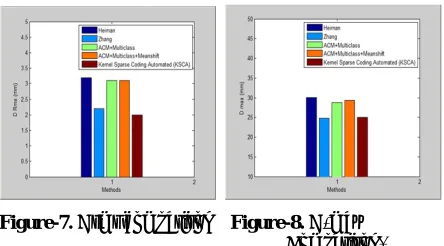
Figure-7. Drms comparison Figure-8. D-max Comparison.
Figure 7 and 8 shows the performance comparison of the Drms and D-max. It is clearly observed from the results that the proposed approach outperforms the existing approaches in terms of Drms and D-max. The values of Drms and D-max of the proposed kernel sparse approach is 2 MM and 25 MM, respectively which is lower than the existing approaches.
Figure-9. Runtime comparison. Figure 10. Accuracy comparison.
Figures 9 and 10 show the performance comparison of runtime and accuracy for different
approaches. It is observed from the Figures that the proposed Kernel sparse coding approach attains 91% accuracy whereas the existing approaches such as Heiman, Zhang, ACM+multi-atlas and ACM+multi-atlas+mean-shift attains the accuracy of 70%, 74%, 79% and 82% respectively. Thus the proposed approach outperforms the other approaches. The run time taken by the proposed kernel sparse coding approach is lower than ACM mulit-atlas mean shift approach. This research work performs fairly in terms of runtime. The future work is to lessen the time consumed by the proposed approach.
CONCLUSIONS
Accurate segmentation of liver tissue from medical images has become an active area of research in medical image processing. This research work aims to develop an efficient liver segmentation approach for computer aided liver disease diagnosis and surgical planning. This paper proposes an efficient kernel sparse coding approach for liver segmentation. The two metrics are used to construct kernel matrices they are pixel intensities and their spatial locations. The intensity matrix and spatial location matrix are combined to construct the ensemble kernel matrix. The kernel dictionary for sparse coding pixels in a nonlinear feature space is also obtained from the kernel matrix. The linear classifier is used to classify the affected regions in the liver. The experimental result shows that the proposed kernel sparse coding technique performs better than other liver segmentation techniques such as Heimen, Zhang, ACM+Multiclass and ACM+Multiclass+Meanshift approach.
REFERENCES
[1] Oussema Zayane1, Besma Jouini1, Mohamed Ali Mahjoubm, “Automatic liver segmentation method in CT images” Canadian Journal on Image Processing and Computer Vision. Vol. 2, No. 8, December 2011.
[2] C-M Wu, Y-C Chen, and K-S Hsieh. “Texture Features for Classification of Ultrasonic Liver Images”. IEEE Trans. Med. Imaging. 11(2): 141-152, 1992.
[3] L. Gao, D. G. Heath, B. S. Kuszyk, and E. K. Fishman. “Automatic liver segmentation technique for three-dimensional visualization of CT data”, Radiology. 201(2): 359-64, 1996.
[4] Daniau-Clavreul P. Y., Roullier V., Cavaromenard C., Segmentation automatique du foiesur des IRM abdominals.
[5] K. Bae, M. Giger, C. Chen, and C. Kahn, Jr., “Automatic segmentation of liver structure in CT images”, Medical Physics.20(1) 1993, 71-78.
[image:8.612.74.296.348.471.2] [image:8.612.74.295.573.681.2]watershed algorithm based on morphological filtering”, SPIE Proc. 5370 (2004) 1658-1666.
[7] M.L. Giger, N. Karssemeijer, S.G. Armato III, Guest editorial: “computer-aided diagnosis in medical imaging”, IEEE Trans. Med.Imaging. 20(12) (2001) 1205-1208.
[8] Seo, K.: “Automatic hepatic tumor segmentation using composite hypotheses”. Image Analysis and Recognition. 3656 (2005) 922-929.
[9] Yim, P., Foran, D.: “Volumetry of hepatic metastases in computed tomography using the watershed and active contour algorithms”. In: Proceedings of the 16th IEEE Symposium on Computer-based Medical Systems. (2003) 329-335.
[10]Lu, R., Marziliano, P., Thng, C.: “Liver tumor volume estimation by semi-automatic segmentation method”. In: Proceedings of the 27th Annual Conference of IEEE Engineering in Medicine and Biology. (2005) 3296-3299.
[11]Zhao, B., Schwartz, L., Jiang, L., Colville, J., Moskowitz, C., Wang, L., Leftowitz, R., Liu, F., Kalaigian, J.: “Shape-constraint region growing for delineation of hepatic metastases on contrast-enhanced computed tomograph scans”. Investigative Radiology. 41(10) (2006) 753-762.
[12]Deng, X., Du, G.: “3D Liver Tumor Segmentation Challenge” 2008, http://lts08.bigr.nl/index.php. (2008).
[13]Hongwei Ji, Jiangping He, Xin Yang, Rudi Deklerck, and Jan Cornelis “ACM-Based Automatic Liver Segmentation from 3D CT Images by Combining Multiple Atlases and Improved Mean Shift Techniques” IEEE Transactions on Information Technology in Biomedicine. 2013.
[14]J.J. Thiagarajan and K.N. Ramamurthy and A. Spanias, “Multilevel dictionary learning for sparse representation of images”, Proceedings of the IEEE DSP Workshop. (2011).
[15]J.J. Thiagarajan and K.N. Ramamurthy and A. Spanias, “Kernel Sparse Models for Automated Tumor Segmentation”, International Journal on Artificial Intelligence Tools. 2013.
[16]D.L. Donoho and M. Elad. “Optimally sparse representation in general (non orthogonal) dictionaries via ℓ1 minimization”, Proceedings of the National Academy of Sciences. 100(5) (2003) 2197-2202.
[17]S.S. Chen and D.L. Donoho and M.A. Saunders, “Atomic decomposition by basis pursuit”, Neural Computation. 43 (1) (2001) 129-159.
[18]H. Lee et al., “Efficient sparse coding algorithms”, Advances in neural information processing systems. 19 (2007) 801.
[19]B. Efron and T. Hastie and I. Johnstone and R. Tibshirani, “Least angle regression”, The Annals of statistics. 32(2) (2004) 407–499.
[20]R. Rubinstein and A.M. Bruckstein and M. Elad, “Dictionaries for Sparse Representation Modeling”, Proceedings of the IEEE. 98 (6) (2010) 1045–1057.
[21]Ramirez and P. Sprechmann and G. Sapiro, “Classification and clustering via dictionary learning with structured incoherence and shared features”, Proceedings of IEEE CVPR. (2010) 3501-3508.
[22]J. Wright et al., “Robust Face Recognition via Sparse Representation”, IEEE Transactions on Pattern Analysis and Machine Intelligence. 31(2) (2001) 210-227.
[23]S. Gao and I. Tsang and L.T. Chia, “Kernel sparse representation for image classification and face recognition”, Proceedings of ECCV. (2010) 1-14.
[24]N. Cristianini and J. Shawe-Taylor, An introduction to support Vector Machines: and otherkernel-based learning methods (Cambridge University Press, 2000).
[25]J.J. Thiagarajan, K.N. Ramamurthy and A. Spanias, “Optimality and Stability of the K-Hyperline Clustering Algorithm”, Pattern Recognition Letters. 32(9) (2011) 1299-1304.
[26]H.V. Nguyen et al., “Kernel Dictionary Learning”, Proceedings of the IEEE ICASSP. (2012).
[27]J.T.Y. Kwok and I.W.H. Tsang, “The pre-image problem in kernel methods”, IEEE Transactions on Neural Networks. 15 (6) (2004) 1517-1525.
[28]Feng GR, Huang G-B, Lin QP et al. (2009). “Error minimized extreme learning machine with hidden nodes and incremental learning”. IEEE Trans Neural Network. 20(8): 1352-1357.
[29]Barlett PL. (1998). “The sample complexity of pattern classification with neural networks: the size of the weights is more important than the size of the network” IEEE Trans Theory. 44(2): 525-536.
[31]M.C. Clark et al., “Automatic tumor segmentation using knowledge-based techniques”, IEEE Transactions on Medical Imaging. 17(2) (1998) 187-201.
[32]Heimann T, VaGinneken B, Styner MA, Arzhaeva Y (2009)“ Evaluation Methods for Liver Segmentation from CT images”. IEEE Transactions on Medical Imaging. 28(8) (2009) 1251-1265.
[33]Daoqiang Zhang, Songcan Chen, “Robust Image Segmentation using FCM with Spatial constraints based on Kernel-Induced Distance Measure”. IEEE Transactions on Systems, Manand Cybernetics. 34(4) (2004).
[34]HongweiJi, Jianping He, Xin Yang, Deklerck R, “ACM Based Automatic Liver Segmentation from 3-D CT images by combining Multiple Atlases and Improved Mean-Shift techniques”. IEEE Journal of Biomedical and Health Informatics. 17(3) (2013) 690-698.