Spatial and temporal variability of rainfall in the Nile Basin

www.hydrol-earth-syst-sci.net/19/2227/2015/ doi:10.5194/hess-19-2227-2015

© Author(s) 2015. CC Attribution 3.0 License.

Spatial and temporal variability of rainfall in the Nile Basin

C. Onyutha1,2and P. Willems1,3

1_{Hydraulics Laboratory, KU Leuven, Kasteelpark Arenberg 40, 3001 Leuven, Belgium} 2_{Faculty of Technoscience, Muni University, P.O. Box 725, Arua, Uganda}

3_{Department of Hydrology and Hydraulic Engineering, Vrije Universiteit Brussel, Pleinlaan 2, 1050 Elsene, Brussel, Belgium} Correspondence to: C. Onyutha ([email protected])

Received: 8 September 2014 – Published in Hydrol. Earth Syst. Sci. Discuss.: 28 October 2014 Revised: 3 February 2015 – Accepted: 10 April 2015 – Published: 8 May 2015

Abstract. Spatiotemporal variability in annual and seasonal rainfall totals were assessed at 37 locations of the Nile Basin in Africa using quantile perturbation method (QPM). To get insight into the spatial difference in rainfall statistics, the sta-tions were grouped based on the pattern of the long-term mean (LTM) of monthly rainfall and that of temporal vari-ability. To find the origin of the driving forces for the tem-poral variability in rainfall, correlation analyses were car-ried out using global monthly sea level pressure (SLP) and sea surface temperature (SST). Further investigations to sup-port the obtained correlations were made using a total of 10 climate indices. It was possible to obtain three groups of stations; those within the equatorial region (A), Sudan and Ethiopia (B), and Egypt (C). For group A, annual rain-fall was found to be below (above) the reference during the late 1940s to 1950s (1960s to mid-1980s). Conversely for groups B and C, the period from 1930s to late 1950s (1960s to 1980s) was characterized by anomalies being above (be-low) the reference. For group A, significant linkages were found to Niño 3, Niño 3.4, and the North Atlantic Ocean and Indian Ocean drivers. Correlations of annual rainfall of group A with Pacific Ocean-related climate indices were in-conclusive. With respect to the main wet seasons, the June– September rainfall of group B has strong connection to the influence from the Indian Ocean. For the March–May (October–February) rainfall of group A (C), possible links to the Atlantic and Indian oceans were found.

1 Introduction

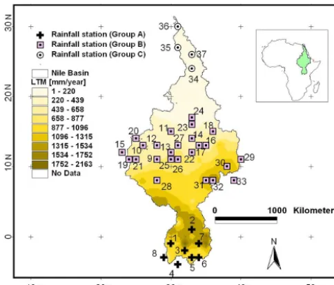
The Nile Basin, which has a total catchment area of about 3 400 000 km2 (see Fig. 1), stretches over 35◦of latitude in

the north–south direction (31◦N–4◦S) and over 16◦of lon-gitude in the west–east direction (24–40◦E). It comprises of the River Nile, which is the world’s longest river under arid conditions and is fed by two main river systems: the White Nile (from the equatorial region) and the Blue Nile (from the Ethiopian highlands). The riparian countries of the Nile Basin include Burundi, Rwanda, Uganda, Kenya, Tanzania, South Sudan, Democratic Republic of Congo, Sudan, Eritrea, Ethiopia, and Egypt. The climate of the Nile Basin is charac-terized by a strong latitudinal wetness gradient (Camberlin, 2009). There is a spatially contrasted distribution of mean annual rainfall over the Nile Basin. About 28 % of the basin receives less than 100 mm annually. Whereas some parts ex-perience hyper-arid conditions, substantial area exhibits sub-humid conditions. Rainfall in excess of 1000 mm is restricted mainly to the equatorial region and the Ethiopian highlands. From northern Sudan all across Egypt, rainfall is negligible (below 50 mm except along the Mediterranean coast). This general distribution reflects the latitudinal movement of the inter-tropical convergence zone (ITCZ) which never reaches Egypt and northern most Sudan, stays only briefly in central Sudan and longer further south (Camberlin, 2009).

ma-Figure 1. Locations of the selected meteorological stations (see Ta-ble 1 for details) in the Nile Basin; the background is based on the long-term mean (LTM) of annual rainfall.

jor concern from water resources managers and policy deci-sion makers. For only the year 2014, a number of studies re-lated to climate variability have been conducted, examples of which include Casanueva et al. (2014), Kummu et al. (2014), Moges et al. (2014), Nachshon et al. (2014), Seiller and An-ctiln (2014), Trambauer et al. (2014), and Verdon-Kidd et al. (2014). Climate variability appears to have a very marked effect on many hydrological series (Kundzewicz and Rob-son, 2004). Among all the atmospheric variables, variability in rainfall is a critical factor in determining the spatiotempo-ral influence of the climate system on hydrology and related water management applications.

Annually, extreme rainfall and associated flooding events inflict severe damage to public life and property in many parts of the world. This is typical to various regions of the Nile Basin. Areas close to the Lake Victoria and generally low-lying parts of the Lake Victoria basin are characterized by episodes of floods, for instance, downstream of Nzoia River and Nyando River, and around the Budalang’i and Kano plains (Gichere et al., 2013). Heavy rainfall events over Khartoum and Atbara led to severe flooding in Sudan during August–September 1988 (Sutcliffe et al., 1989). According to Nawaz et al. (2010), the prolonged drought in the Greater Horn of Africa that ended in 2005 was followed by severe flooding in August 2006. In the history of flooding in the Nile Basin, Ethiopia, Tanzania, Kenya, Sudan, and Uganda are the most affected countries in terms of the average number of flooding occurrences (Kibiiy et al., 2010). The flood dam-ages in the Nile Basin are exacerbated by the already existing crisis of widespread poverty associated with frenzied popu-lation growth, and thus the need for sustainable planning, de-sign, and management of risk-based water resources

applica-tions. To do so, it is important to study the historical temporal variability in rainfall, and associated possible driving forces which might be from large-scale ocean–atmosphere interac-tions, anthropogenic factors as well as the influence from re-gional features such as water bodies, topography, etc. Clear representation of spatial differences in the rainfall statistics across the study area would also be very supportive.

and rain-fed agriculture, together with high rainfall variabil-ity is one of the main causes of food insecurvariabil-ity and the most daunting challenge the entire Nile Basin faces (Melesse et al., 2011).

This paper is aimed at analyzing spatiotemporal variabil-ity of rainfall over the Nile Basin while investigating any linkages to large-scale ocean–atmosphere interactions. This is done at both seasonal and annual scales. Inter-annual vari-ability of rainfall volumes at such timescales is important for various types of water and agricultural management prac-tices. It is important to note that for brevity in this paper, only the rainfall variability driving forces from the large-scale ocean–atmosphere interactions (but not the influence from anthropogenic factors or regional features) were con-sidered.

2 Data and considerations 2.1 Rainfall

Monthly data were obtained from the Food and Agricul-ture Organization, FAO (2001), agro-climatic database using FAOCLIM 2 tool obtainable from http://www.fao.org/ (ac-cessed January 2010). FAOCLIM contains monthly world wide agro-climatic data for 28 100 stations with up to 14 ob-served and computed agro-climatic variables. To enhance the acceptability of the research findings, long-term rainfall se-ries of length not less than 40 years and missing data points not more than 10 % were used. However, to check on the spa-tial coherence of the variability results across the study area, a period of not less than 35 years over which each station had rainfall data was considered. This was done because of the spatial coherence of the temporal variability results that could be obtained on a regional basis when data from the different meteorological stations are of the same length and picked over the same time period for analysis.

A number of potential data problems, for instance missing values, data entry errors, outliers, etc., were solved by careful inspection. The data were screened and comparisons between stations were made using the statistical metrics coefficient of variation (Cv), skewness (Cs), and actual excess kurtosis (Ku). Missing data were filled in using the inverse distance-weighted (IDW) interpolation technique of Shepard (1968). The missing rainfall intensity (PX) at station X for a certain period using rainfall values (Pj) atgneighboring stations for the same period is given by

PX=

g

X

j=1

Pj·d_j−r g

X

j=1

d_j−r

!−1

, (1)

wheredj is the distance between stationX(the one with the missing record) and that in the neighborhood being used for interpolation, andris the power parameter (an arbitrary pos-itive real number).

The IDW approach has been applied to climate data such as rainfall in a number of studies, e.g., by Ahrens (2006), Legates and Willmott (1990), and Rudolf and Rubel (2005). It is important to note that the reliability of the IDW in-terpolation lies in the value ofr. A small value ofr tends to approximate the interpolated record to averages of the neighboring stations used, while a larger value ofr weighs down points further away and assigns larger weights to the nearest points (Lu and Wong, 2008). According to Dirks et al. (1998), interpolation errors appear to be minimized by takingr=2 for daily or monthly data,r=3 for hourly and

r=1 for annual data. However, following Goovaerts (2000) and Lloyd (2005), r is usually set to 2. Hence r=2 was adopted in this study.

From the monthly rainfall series, seasonal and annual rain-fall intensity totals were obtained for the analysis of tempo-ral variability. Table 1 shows for all the stations the coor-dinates, station name, station ID, record length, long-term mean (LTM; mm year−1),Cv,Cs, andKuof the annual rain-fall time series. Since for a normal distribution it is expected that Cs=0 and Ku=0, it can be said that the data at the selected stations are, on average, slightly positively skewed (Cs=0.85) and leptokurtic (Ku=2.24), i.e., compared with normal distribution, its central peak is higher and sharper and its tails are longer and fatter. TheCvranges from 0.11 (station 30) to 1.95 (station 35) which shows that there is considerably moderate variability on a year to year basis in the study area. The LTM of the annual rainfall varies from 1.2 mm year−1(station 34) to 2163 mm year−1(station 32). Generally, the latitudinal decrease in the rainfall statistics from upstream to downstream of the River Nile is also re-flected in the higher magnitude of the runoff values and its stronger variability in the southern rather than the northern part (Nyeko-Ogiramoi et al., 2012).

2.2 Large ocean–atmospheric-related series

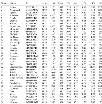
Table 1. Overview of selected stations and their annual rainfall data.

St. no. Station ID Long. Lat. From To Cv Cs Ku LTM

1 Kabale UG19KBL0 29.98 −1.25 1917 1993 0.17 0.49 0.07 1002.6 2 Namasagali UG12NMSG 32.93 1.00 1915 1978 0.19 1.89 6.12 1255.7 3 Igabiro TZ11GBR0 31.53 −1.78 1931 1982 0.24 0.82 0.80 1197.6 4 Kibondo TZ30KBND 30.68 −3.57 1926 1978 0.29 2.47 9.50 1209.1 5 Ngudu TZ23NGD0 33.33 −2.93 1928 1971 0.33 1.61 3.88 870.1 6 Shanwa TZ33SHNW 33.75 −3.15 1931 1985 0.24 0.68 0.28 829.0 7 Tarime TZ14TRM0 34.37 −1.35 1933 1975 0.20 1.48 1.94 1474.7 8 Bujumbura BI39BJMB 29.32 −3.32 1930 2004 0.18 0.27 0.09 251.4 9 El-Da-Ein SD16LDN0 26.10 11.38 1943 1990 0.27 0.17 −0.03 473.7 10 El-Fasher SD35LFSH 25.33 13.62 1917 1996 0.43 1.22 1.92 260.5 11 El-Obeid SD30LBD0 30.23 13.17 1902 1996 0.32 0.53 0.39 355.9 12 En-Nahud SD28NNHD 28.43 12.70 1911 1996 0.28 0.39 1.00 384.1 13 Er-Rahad SD20RRHD 30.60 12.70 1931 1984 0.31 0.80 3.21 431.9 14 Fashashoya SD32FSHS 32.50 13.40 1946 1988 0.32 0.04 −0.11 297.4 15 Garcila SD23GRCL 23.12 12.35 1943 1986 0.30 1.97 6.75 671.6 16 Hawata SD34HWT0 34.60 13.40 1941 1988 0.23 −0.19 1.35 571.2 17 Jebelein SD22JBLN 32.78 12.57 1927 1988 0.29 −0.50 −0.40 377.4 18 Kassala SD56KSSL 36.40 15.47 1901 1996 0.30 −0.04 −0.18 297.8 19 Kubbum SD13KBBM 23.77 11.78 1943 1985 0.27 −0.01 −0.23 645.5 20 Kutum SD44KTM0 24.67 14.20 1929 1990 0.40 0.16 0.28 288.1 21 Nyala SD24NYL0 24.88 12.05 1920 1996 0.29 0.11 −0.30 439.5 22 Renk SD12RNK0 32.78 11.75 1906 1987 0.20 0.35 −0.09 507.5 23 Shambat-Obs. SD52SHMB 32.53 15.67 1913 1993 0.94 2.99 11.31 166.5 24 Shendi SD63SHND 33.43 16.70 1937 1990 0.74 1.16 2.08 100.1 25 Talodi SD01TLD0 31.38 10.60 1916 1987 0.23 1.12 3.57 791.5 26 Talodi-M-Agr. SD00TLDM 30.50 10.60 1942 1985 0.21 0.41 −0.35 774.2 27 Umm-Ruwaba SD21MMRW 31.20 12.80 1912 1989 0.32 1.93 9.26 365.3 28 Wau SD78W000 28.02 7.70 1904 1990 0.16 0.26 −0.34 1109.8 29 Combolcha ET19KMBL 39.72 11.08 1952 1996 0.17 −0.84 0.69 1031.8 30 Debremarcos ET07DBRM 37.72 10.35 1954 1998 0.11 0.82 0.59 1335.4 31 Gambela ET84GMBL 34.58 8.25 1905 1993 0.22 0.00 0.25 1244.6 32 Gore ET85GR00 35.55 8.17 1946 1996 0.20 1.40 2.15 2163.0 33 Wenji ET89WNJ0 39.25 8.42 1951 1994 0.28 −0.76 1.92 786.9 34 Asswan EG32SSWN 32.78 23.97 1935 1986 1.92 2.15 3.77 1.2 35 Asyut EG71SYT0 31.17 27.20 1925 1986 1.95 2.50 5.86 1.9 36 Helwan EG91HLWN 31.33 29.87 1904 1988 0.72 1.39 2.07 25.7 37 Qena EG62QN00 32.72 26.15 1935 1986 1.78 2.17 4.11 2.4

Long.: longitude (◦_{); Lat.: latitude (}◦_{); LTM: long-term mean.}

2.2.1 SLP and related series

1. The global monthly historical SLP (HadSLP2) data (Allan and Ansell, 2006) from reconstruction of land and marine observations were obtained from the NOAA/OAR/ESRL PSD, Boulder, Colorado, USA (see Table 2).

2. The North Atlantic Oscillation (NAO) is the normal-ized SLP difference between SW Iceland (Reykjavik), Gibraltar, and Ponta Delgada (Azores). The NAO (Hur-rell, 1995; Jones et al., 1997) was obtained from the Cli-matic Research Unit (CRU).

3. The North Pacific Index (NPI) is the area-weighted SLP over the region 30–65◦_{N, 160}◦_E–140◦_{W. The NPI} (Trenberth and Hurrell, 1994) was obtained from the National Centre for Atmospheric Research/University Corporation for Atmospheric Research.

4. The trans-polar index (TPI) is defined as the normal-ized pressure difference between Hobart, Australia and Stanley, Falkland Islands. The TPI (Jones et al., 1999; Pittock, 1980, 1984) was obtained from the CRU. 5. The Southern Oscillation index (SOI) is defined as the

Table 2. Overview of SLP, SST and related time series.

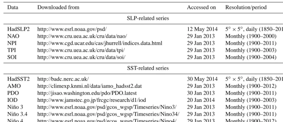
Data Downloaded from Accessed on Resolution/period

SLP-related series

HadSLP2 http://www.esrl.noaa.gov/psd/ 12 May 2014 5◦×5◦, daily (1850–2013) NAO http://www.cru.uea.ac.uk/cru/data/nao/ 29 Jan 2013 Monthly (1900–2000) NPI http://www.cgd.ucar.edu/cas/jhurrell/indices.data.html 29 Jan 2013 Monthly (1900–2011) TPI http://www.cru.uea.ac.uk/cru/data/tpi/ 29 Jan 2013 Monthly (1900–2003) SOI http://www.cru.uea.ac.uk/cru/data/soi/ 29 Jan 2013 Monthly (1900–2004)

SST-related series

HadSST2 http://badc.nerc.ac.uk/ 30 May 2014 5◦×5◦, daily (1850–2013) AMO http://climexp.knmi.nl/data/iamo_hadsst2.dat 29 Jan 2013 Monthly (1900–2012) PDO http://jisao.washington.edu/pdo/PDO.latest 30 Jan 2013 Monthly (1900–2011) IOD http://www.jamstec.go.jp/frcgc/research/d1/iod 20 Jan 2014 Monthly (1900–2003) Niño 3 http://www.esrl.noaa.gov/psd/gcos_wgsp/Timeseries/Nino3/ 29 Jan 2013 Monthly (1900–2011) Niño 3.4 http://www.esrl.noaa.gov/psd/gcos_wgsp/Timeseries/Nino34/ 29 Jan 2013 Monthly (1900–2011) Niño 4 http://www.esrl.noaa.gov/psd/gcos_wgsp/Timeseries/Nino4/ 29 Jan 2013 Monthly (1900–2012)

2.2.2 SST and related series

1. The global monthly historical SST (HadSST2) anoma-lies with respect to the 1961–1990 climatology (Rayner et al., 2006) were obtained from the UK Met Office through the British Atmospheric Data Centre.

2. The Atlantic Multidecadal Oscillation (AMO) index is defined as the SST averaged over 25–60◦_{N, 7–70}◦_W minus the regression of this SST on global mean tem-perature (van Oldenborgh et al., 2009). The AMO index was obtained from the Koninklijk Nederlands Meteo-rologisch Instituut through their climate explorer. 3. The Pacific decadal oscillation (PDO) index is the

lead-ing principal component of North Pacific monthly SST variability (poleward of 20◦N in the Pacific Basin). The digital values of the PDO index of Mantua et al. (1997) were obtained from the database of the Joint Institute for the Study of the Atmosphere and Ocean.

4. The Indian Ocean dipole (IOD) is the anomalous SST difference between the western (50–70◦E and 10◦S– 10◦N) and the south eastern (90–110◦E and 10◦S– 0◦N) equatorial Indian Ocean. The IOD series was ob-tained from the Japan Agency for Marine-Earth Science and Technology.

5. Area averaged Niño SST indices (Rayner et al., 2003; Trenberth, 1997) for the tropical Pacific regions de-scribed by Niño 3 (90–150◦W and 5◦N–5◦S), Niño 3.4 (120–170◦W and 5◦N–5◦S), and Niño 4 (150◦W– 160◦E and 5◦N–5◦S) were obtained from the Earth System Research Laboratory of the National Oceanic and Atmospheric Administration.

PDO, IOD, AMO, and SOI have been used in recent studies on rainfall variability in two sub-regions of the Nile Basin by Moges et al. (2014) and Taye and Willems (2012) for Ethiopia, and Nyeko-Ogiramoi et al. (2013) for the Lake Vic-toria basin.

3 Methodology

3.1 Computing rainfall variability using the quantile perturbation method

The QPM is analogous to one of the methods for deriving cli-mate change scenarios or for propagating clicli-mate change sig-nals to historical observations by perturbing these series us-ing information from climate model runs (see Mpelasoka and Chiew, 2009; Willems and Vrac, 2011). In a number of stud-ies including Chiew (2006), Harrold et al. (2005), and Har-rold and Jones (2003), the quantile mapping method, which QPM makes use of, was used to scale ranked historical daily rainfall quantiles in quantile dependent methods to establish future climate change scenarios.

When applied to historical series, as is done in this study, the QPM considers changes in quantiles with similar ex-ceedance frequency or return periodT compared from two time series. One of the series is taken to be the complete time series, while the other is a time slice of the entire historical period. A block size (time slice) of lengthD (in years) is selected for a given hydrometeorological variable of histori-cal period,nyears. Let us call the time slice series variable

x, and the full time seriesy. By takingj as the rank of the variable extreme and computing the empiricalT as (D/j) forxand (n/j) fory, the values of the extremes are ranked in such a way that forj=1,2,3, . . .N we have the highest

etc. forx and correspondinglyy(n/1),y(n/2),y(n/3)etc. for y. In the next step, the quantiles of x andy with simi-lar Ts are compared. In some cases, linear interpolations are carried out for (n/j) to locate it between (D/j) values when these empirical Ts do not match. Finally, the relative change or perturbation factor on the quantiles is calculated as a ratio of the block period extremesx(D/j )and those of the base-line periody(n/j ). The ultimate anomaly value for each time slice period is obtained as the average value of the perturba-tion factors found at previous step. Eventually, the variaperturba-tion in the extreme quantiles in the time slice over the full time se-ries is represented by a single anomaly value. This procedure is repeated by moving the time slice forward by one time step. The time step in this study was taken as one year. At the end of it all, a complete analysis accounting for all possible times is obtained from the repeated process of moving slice over the entire time series.

It is well known that the estimation of Ts from small sam-ple series can be characterized by bias. This bias becomes large when theT being estimated (by extrapolation after fit-ting theoretical distribution in the frequency analysis) is far higher than the data record length. To ensure that the bias in the anomalies computed over each time slice does not signif-icantly affect the QPM variability results, extrapolations are avoided. This is done by considering only the empirical Ts, i.e., Ts not greater thanD(for each time slice) orn(for the full series).

Due to sensitivity of the QPM to block length (i.e., a sub-series of the full time sub-series covering the period of interest), preliminary analysis was conducted using block periods of 5, 10, and 15 years (Fig. 2a). It is important to note that the choice of the block length is subjective and may depend on the objective of the study. It can be noted from Fig. 2a that the computed anomalies are over-/underestimated for lower than higher time slice. Furthermore, as the block length increases, the pattern of persistence in the rainfall quantiles becomes smoother or clearer. A block length of 15 years was found to give a much clearer oscillation pattern in the rainfall data than for 5 and 10 years, and was eventually adopted for this study. Alongside details on the QPM, the selection and sen-sitivity of the block length can be found fully discussed by Ntegeka and Willems (2008) and/or Willems (2013).

To understand the variability in rainfall intensity and/or the driving forces, the QPM was applied to

1. series of annual rainfall totals and mean of SLP, SST, or related variables in each year;

2. series of seasonal rainfall totals and mean of SLP, SST, or related variables in each season.

3.2 Test of significance

The null hypothesis (H0) that the observed temporal variabil-ity in the rainfall data set in question is caused by only nat-ural variability or randomness (i.e., there is no persistence in

Figure 2. QPM results at station 7 for the period 1935–1970 us-ing time slice(s) (a) considered in sensitivity analysis (5, 10 and 15 years), and (b) selected for the study (15 years).

the temporal climate variation) was considered. To verify the said hypothesis at 5 % level of significance, nonparametric bootstrapping Monte Carlo simulations were used to test the statistical significance of the temporal variation. Some of the common approaches that exist to construct confidence inter-vals (CIs) in statistical hypothesis testing include the Monte Carlo technique, and the Jackknife method (Tukey, 1958). Examples of Monte Carlo simulations applied in statistical modeling can be found in much of the literature (Beersma and Buishand, 2007; Chu and Wang, 1998; Davidson and Hinkley, 1997; Onyutha and Willems, 2013). Other statisti-cal approaches of uncertainty assessment can be found elab-orated in Montanari (2011). To derive bounds of variabil-ity using 95 % CI, the nonparametric bootstrapping method (Davidson and Hinkley, 1997) was employed as follows:

1. The original full time series is randomly shuffled to ob-tain a new temporal sequence.

2. The new series is divided to obtain subseries each of length equal to the time slice period.

3. New temporal variation of anomalies is obtained by ap-plying QPM to the shuffled series.

4. Steps 1, 2, and 3 are repeated 1000 times to obtain 1000 anomaly factors for each subseries.

6. The limits (upper, lower) of the 95 % CI for each time moment are taken as the (25th, 975th) anomaly values. Figure 2 shows an example of annual rainfall quantile anomaly series (QPM results) for station 7. The annual rain-fall series is included in Fig. 2b to visualize the pattern of the quantile anomaly values in reference to the original time series. The up and down arrows indicate periods of oscilla-tion high, OH (1940–1955), and oscillaoscilla-tion low, OL (1956 to mid-1960s), respectively. Since the upper 95 % CI limit is up crossed by the anomaly values in the OH period, it means that the OH is statistically significant in the rainfall of the selected station.

3.3 Spatial differences in rainfall statistics

Differences between rainfall intensity at the selected stations were assessed in terms of patterns of their long-term monthly mean and temporal variability. For each month in the entire series, an average of the rainfall was calculated. By repeating the procedure for all the months, indication of which months fall in the wet or dry seasons was obtained. Graphically, sim-ilarity in the obtained patterns was compared jointly for rain-fall from all the stations. The temporal patterns of anomaly (QPM results) in the rainfall of the different selected stations were also compared. This was also graphically carried out by examining the similarities in the co-occurrences of the OHs and OLs. Strong spatial differences of these rainfall statis-tics could indicate difference in possible driving forces of temporal variability across the study area. It can also help to indicate the period during which a particular region is char-acterized by dry or wet spells.

3.4 Correlation between changes in rainfall and anomalies in SLP, SST, and/or climate indices Any possible linkage of rainfall variability to large-scale ocean–atmosphere interactions was sought using correlation analysis (at significance level of 5 and 1 %) under the null hypothesisH0that there is no correlation between the rafall QPM results and those of the SLP, SST or climate in-dices. To locate the part of the world over which the driv-ing influence for temporal variability in rainfall over the Nile Basin originates, correlation between the regional or basin-wide annual/seasonal total rainfall QPM results and corre-sponding SLP or SST at each grid point was calculated. Next to the correlation with the SLP, also the correlation with SLP differences, being a measure of atmospheric circulation, was tested. For that purpose, the SLP difference were considered over any two regions with significant correlations but of op-posite signs and for which it is expected that the related at-mospheric circulation drives the rainfall over the region un-der study. The oscillation pattern of the SLP difference was compared with that of the regional/basin-wide rainfall total. To further confirm the results of the comparison, correla-tion analyses between the QPM results of stacorrela-tion-based

an-nual/seasonal rainfall and those of climate indices were car-ried out. Correlations between rainfall QPM results and those of the climate indices were analyzed for further investigation.

4 Results and discussions

4.1 Spatial differences in rainfall statistics

Figure 3 shows long-term mean monthly rainfall pattern for the selected stations. It is shown that the rainfall at stations in the equatorial region (group A) exhibit bimodal patterns with the main wet season in March–May (MAM) and “short rains” in October–December (OND) (Nicholson, 1996). The main wet season over Sudan and Ethiopia (group B) occurs in the months of June–September (JJAS). For stations in Egypt (group C), it is seen that the long-term mean monthly rain-fall values are far lower (and of more unclear patterns) than those in groups A and B. However, it can be seen that the wet seasons cover MAM and the period of October–February (ONDJF). Because the rainfall totals for ONDJF are larger than those for MAM, it was taken as the main wet season for variability analysis. According to Camberlin (2009), large variations in long-term mean rainfall statistics across the Nile Basin are due to its great latitudinal and longitudinal extents. Based on Fig. 3, it was possible to group the selected sta-tions into three: those in the equatorial region (group A), Su-dan and Ethiopia (group B), and Egypt (group C). Validation of the grouping of the rainfall stations was in terms of the temporal variability patterns as shown next.

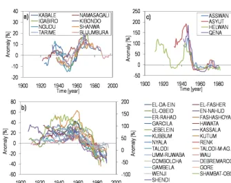
Figure 4 shows temporal variability of quantile anomaly (QPM results) for annual rainfall at the different stations of each group. Just like for the long-term mean monthly rain-fall, it is shown that these general patterns of the temporal variability at stations of each group are similar (Fig. 4).

Figure 3. Long-term mean monthly rainfall pattern for group (a) A, (b) B, and (c) C.

Figure 4. QPM results for annual rainfall using a time slice of 15 years and rainfall stations for group (a) A, (b) B, (c) C.

on only station 36 whose record starts in 1904. The OH oc-curred in the period from about 1940 to early 1950s. This was significant at stations 34–35 and 37. Though not significant

were significant OHs like for the annual rainfall (over the same period) were 2, 4, and 7 (MAM); 22–23, 26–27, and 32 (JJAS); 35–37 (ONDJF). However, there were some stations that exhibited significant OHs in the main wet season but not for the annual rainfall. These included stations 3 and 8 (for MAM rainfall of group A), 13, and 17 (for JJAS rainfall of group B). The OLs of the main seasons were insignificant at most stations except 18 and 20 over the periods 1922–1933 and 1920–1922, respectively.

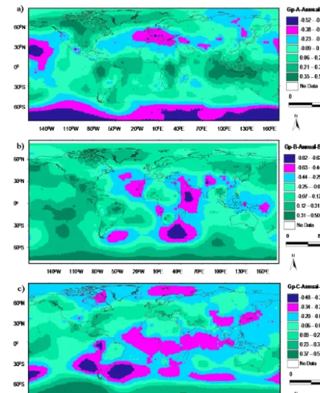
4.2 Identification of drivers for the rainfall variability Figure 5 shows locations over which possible influences for temporal variability of rainfall quantiles (QPM results) in the Nile Basin originate as determined using HadSPL2 data. For the spatial coherence of the driving forces of rainfall variabil-ity, correlations for groups A to C are obtained over the pe-riods in which each station had data records i.e., 1935–1970, 1954–1992, and 1945–1985. Eventually, the critical values of the correlation coefficients at significance level of 5 % (1 %) for groups A–C are 0.33 (0.41), 0.32 (0.41), and 0.31 (0.41). For group A, it is shown in Fig. 5a that the quantile anomalies of the region-wide annual rainfall are correlated to that of the annual SLP in the Indian Ocean and North America (positively), and Pacific Ocean and Southern Ocean (around Antarctica) (negatively). For group B, it is shown that the annual rainfall variability is positively linked to SLP at the Pacific Ocean, and negatively to that at the Indian Ocean. This correlation is highly consistent with the find-ings of Taye and Willems (2011) for the annual rainfall over the Ethiopian highlands. According to Camberlin (1997) the part of the Nile Basin that receives the summer rains, i.e., JJAS season, has a strong connection with the Indian mon-soon. A deepened monsoon low increases the pressure gradi-ent with the South Atlantic Ocean, resulting in strengthened moist south-westerlies/westerlies over Ethiopia, Sudan, and Uganda (Camberlin, 2009). The tropical easterly jet associ-ated with the intense Indian monsoon is another factor, espe-cially for the rainfall over the Sahelian belt (Grist and Nichol-son, 2001). For group C, negative correlations can be seen in around the southern part of Latin America (i.e., southern Atlantic Ocean, and Pacific Ocean); however, positive corre-lations are obtained with influence from the Southern Ocean (near Antarctica), and though over a small area, also in the central Pacific Ocean.

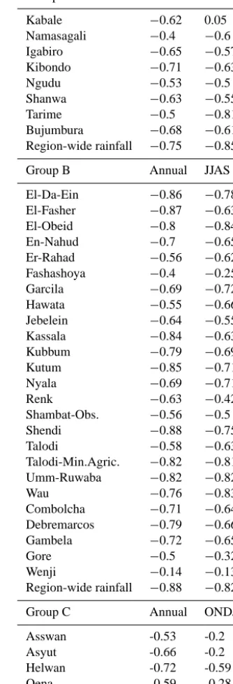
Figure 6 shows oceanic regions with the variability of their HadSST2 series correlated to that of the annual rainfall over the Nile Basin. It is shown that positive influences for annual rainfall variability in the equatorial region originate from the Pacific, Atlantic, and Indian oceans. For stations in groups B and C, correlations in similar oceanic locations are noted but with opposite sign to those in group A. For rain-fall stations in Sudan and Ethiopia, it is important to note that the correlation signs over North Atlantic and South Pa-cific are opposite. This is because rainfall variability of the

Figure 5. Correlation between anomaly in annual sea level pressure (SLP) and that in region-wide annual rainfall for group (a) A, (b) B, (c) C. In the legend, Gp denotes group.

northern and southern zones of Ethiopia are enhanced by an AMO and PDO SST pattern in warm and cool phase respec-tively (Jury, 2010). For the equatorial region, it is shown that significant positive driving forces originate from the Pacific and southern Indian oceans. These locations are consistent to those indicated by Lyon and DeWitt (2012) and Williams and Funk (2011) from where influences on the rainfall vari-ability over the equatorial region originate. However, Tier-ney et al. (2013) showed that it is mainly the Indian Ocean SST which drives East African rainfall variability by alter-ing the local Walker circulation, whereas the influence of the Pacific Ocean is minimal. For Sudan, Ethiopia, and Egypt, it is shown that the SSTs from southern parts of the Indian and Pacific oceans exhibit negative influence on the rainfall variability. These areas with negative correlations in Fig. 6b and c lie from 30 to 60◦_{S, and above 30}◦_{S, respectively.} The negative correlation between Indian Ocean SST and an-nual rainfall over Sudan and Ethiopia as seen in Fig. 6b was also found in a number studies some of which include Ko-recha and Barnston (2007), Osman and Shamseldin (2002), and Seleshi and Demarée (1995).

Figure 6. Correlation between annual sea surface temperature (SST) and that in region-wide annual rainfall for group (a) A, (b) B, (c) C. In the legend, Gp denotes group.

rainfall in the main wet seasons of the different groups, spa-tial maps are shown in Figs. A1 and B1.

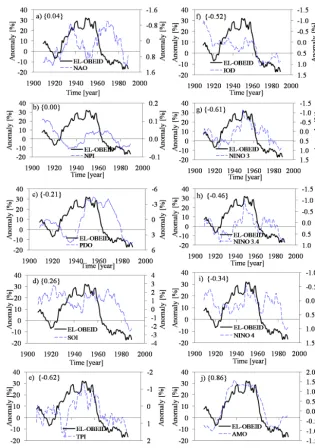
Figure 7 shows temporal patterns of rainfall at selected stations of each group and SLP differences. The locations over which the SLP differences were taken were those with significant correlations but of opposite signs. According to Nicholson (1996), the wind and pressure patterns controlling the rainfall over the equatorial region include a number of major airstreams and convergence zones. The airstreams in-clude the northeast and southeast monsoons which are rel-atively dry (unlike the SW monsoon of Asia), and the con-trastingly humid Congo airstream with westerly and south-westerly flow. The convergence zones include the ITCZ, the Congo Air boundary, and the zone that separates the dry, stable, northerly flow of Saharan origin and the moist southerly flow. In line with the above, the SLP differences were deemed to be taken at locations which fall on either side of the Nile Basin, e.g., between Indian and Atlantic oceans, or Indian and Pacific oceans.

For the same locations shown in Fig. 7a–f, the values of the correlation between the SLP differences and rainfall for the different groups are shown in Table 3. The critical values of the correlation coefficients in Fig. 7 and Table 3 are similar

Table 3. Correlation between rainfall and SLP differences taken at locations shown in Fig. 7.

Group A Annual MAM

Kabale −0.62 0.05 Namasagali −0.4 −0.6 Igabiro −0.65 −0.57 Kibondo −0.71 −0.63 Ngudu −0.53 −0.5 Shanwa −0.63 −0.55 Tarime −0.5 −0.81 Bujumbura −0.68 −0.61 Region-wide rainfall −0.75 −0.85

Group B Annual JJAS

El-Da-Ein −0.86 −0.78 El-Fasher −0.87 −0.63 El-Obeid −0.8 −0.84 En-Nahud −0.7 −0.65 Er-Rahad −0.56 −0.62 Fashashoya −0.4 −0.25 Garcila −0.69 −0.72 Hawata −0.55 −0.66 Jebelein −0.64 −0.55 Kassala −0.84 −0.63 Kubbum −0.79 −0.69 Kutum −0.85 −0.71 Nyala −0.69 −0.71 Renk −0.63 −0.42 Shambat-Obs. −0.56 −0.5 Shendi −0.88 −0.75 Talodi −0.58 −0.63 Talodi-Min.Agric. −0.82 −0.81 Umm-Ruwaba −0.82 −0.82 Wau −0.76 −0.83 Combolcha −0.71 −0.64 Debremarcos −0.79 −0.66 Gambela −0.72 −0.65 Gore −0.5 −0.32 Wenji −0.14 −0.13 Region-wide rainfall −0.88 −0.82

Group C Annual ONDJF

Asswan -0.53 -0.2 Asyut -0.66 -0.2 Helwan -0.72 -0.59 Qena -0.59 -0.28 Region-wide rainfall -0.72 -0.59

Figure 7. Annual SLP differences and rainfall at selected stations of the different groups A–C for a time slice of 5 years; the group labels are in[ ]. The label of a legend indicates the coordinates (degree longitude and latitude) from where the SLP differences were taken. The label in { }show the locations where the coordinates are found. Annual and seasonal timescales are shown in charts (a)–(c) and (d)–(f), respectively.

Figure 8 shows QPM results for a time slice of 15 years in the annual rainfall at station 32 and those for climate in-dices or time series over the period 1902–1996. It is shown for the selected station 32 of group B that the primary influ-ence is from the Atlantic Ocean as exhibited by the AMO index. This is confirmed by the correlation coefficients for all the group stations being positive and significant at sig-nificance levels of both 5 and 1 %. According to Taye and Willems (2012) and Moges et al. (2014), the changes in the Pacific and Atlantic oceans are the major natural causes of the variability in the annual rainfall over the Blue Nile Basin of Ethiopia. For the case of the AMO index, this is consis-tent, for the entire group B, with the finding of this study. However, for the influence from Pacific Ocean (in terms of PDO and SOI), it can be seen from Table 4 that the cor-relation coefficients for stations 11–12, 25 and 27 in Su-dan are rather low. This could be because of the difference in regional influence from features such as topography, wa-ter bodies, or transition in land cover and/or use. Accord-ing to Nicholson (1996), the highlands of the Rift Valley block the moist, unstable westerly flow of the Congo air from reaching the coastal areas (especially of Ethiopia) leading

to complex pattern of rainfall over the Ethiopian highlands. For group B, it is also shown from Table 4 that influences also are obtained from Niño 3, the Indian Ocean and as far as the extra-tropical Southern Hemisphere. The annual rain-fall in Sudan and Ethiopia (group B) has been shown in a number of studies to be influenced by the El Niño–Southern Oscillation (ENSO); see Osman and Shamseldin (2002) for Sudan; Fontaine and Janicot (1992), and Grist and Nichol-son (2001) for the Sahel belt; Abtew et al. (2009), Beltrando and Camberlin (1993), Diro et al. (2010), Korecha and Barn-ston (2007), Seleshi and Demarée (1995), Segele and Lamb (2005), and Seleshi and Zanke (2004) for Ethiopia.

Figure 8. QPM results for annual rainfall and climate indices; the correlation coefficient between the two curves of each chart is labeled in { }.

the equatorial region have been even documented by Indeje et al. (2000), Nicholson (1996), Nicholson and Entekhabi (1986), Ogallo (1988), Nicholson and Kim (1997), Philipps and McIntyre (2000), Ropelewski and Halpert (1987), and Schreck and Semazzi (2004). The link between rainfall over the equatorial region and the Indian Ocean was also found by Camberlin (1997) and Tierney et al. (2013). Nyeko-Ogiramoi et al. (2013) found that variability in the rainfall extremes in the Lake Victoria basin (within the equatorial region) is also linked to the influence from the Pacific Ocean. However, as seen from Table 4, the influences from the Pacific Ocean are not very conclusive with respect to the correlations of NPI,

PDO, and SOI. The inconclusiveness of the correlations for group A and Pacific Ocean-related indices, instead agrees with the remark of Tierney et al. (2013) as already pointed out for Fig. 6.

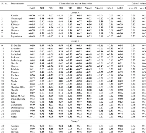
Table 4. Correlation between QPM results for annual rainfall and climate indices over the periods 1935–1970 (for group A), 1954–1992 (for group B) and 1945–1985 (for group C).

St. no. Station name Climate indices and/or time series Critical values

NAO NPI PDO SOI TPI IOD Niño 3 Niño 3.4 Niño 4 AMO α=5 % α=1 %

Group A

1 Kabale −0.70 −0.13 0.07 −0.33 0.29 0.54 0.04 −0.04 0.03 −0.23 0.25 0.33

2 Namasagali −0.64 0.48 −0.49 0.08 0.15 0.60 −0.22 −0.12 −0.18 −0.32 0.28 0.37

3 Igabiro −0.88 0.30 −0.16 0.40 0.81 0.77 0.59 0.50 0.16 −0.91 0.32 0.41

4 Kibondo −0.85 0.00 0.12 0.21 0.67 0.67 0.56 0.53 0.31 −0.79 0.32 0.41

5 Ngudu −0.84 −0.43 0.56 −0.25 0.63 −0.16 0.83 0.89 0.79 −0.40 0.36 0.46

6 Shanwa −0.78 0.25 −0.19 0.36 0.76 0.72 0.62 0.50 0.09 −0.87 0.31 0.40

7 Tarime −0.81 0.56 −0.38 0.43 0.58 0.42 0.49 0.60 0.28 −0.90 0.37 0.47

8 Bujumbura −0.49 0.25 −0.17 0.19 0.40 0.40 0.25 0.18 −0.05 −0.81 0.25 0.34

Group B

9 El-Da-Ein 0.59 0.69 −0.76 0.53 −0.87 −0.83 −0.88 −0.61 −0.36 0.94 0.34 0.44

10 El-Fasher −0.01 0.42 −0.41 0.67 −0.56 −0.80 −0.51 −0.23 −0.33 0.75 0.24 0.32

11 El-Obeid 0.05 0.00 −0.21 0.26 −0.62 −0.52 −0.61 −0.46 −0.34 0.86 0.22 0.30

12 En-Nahud 0.02 0.07 −0.20 0.51 −0.53 −0.79 −0.48 −0.30 −0.34 0.84 0.23 0.31

13 Er-Rahad 0.44 0.26 −0.22 0.08 −0.62 −0.78 −0.59 −0.22 −0.07 0.76 0.31 0.41

14 Fashashoya 0.08 0.81 −0.82 0.59 −0.77 −0.68 −0.72 −0.09 0.10 0.77 0.37 0.47

15 Garcila 0.62 0.69 −0.81 0.42 −0.81 −0.80 −0.88 −0.51 −0.17 0.91 0.36 0.46

16 Hawata 0.41 0.71 −0.76 0.51 −0.84 −0.70 −0.78 −0.43 −0.22 0.85 0.34 0.44

17 Jebelein 0.11 0.26 −0.18 0.25 −0.46 −0.67 −0.45 0.01 0.20 0.81 0.29 0.37

18 Kassala 0.27 0.48 −0.24 0.56 −0.45 −0.80 −0.51 −0.39 −0.53 0.39 0.22 0.30

19 Kubbum 0.76 0.61 −0.75 0.23 −0.86 −0.90 −0.83 −0.45 −0.14 0.96 0.37 0.47

20 Kutum 0.19 0.43 −0.41 0.46 −0.69 −0.75 −0.68 −0.26 −0.08 0.81 0.29 0.37

21 Nyala −0.27 0.32 −0.33 0.81 −0.35 −0.70 −0.43 −0.21 −0.43 0.62 0.25 0.33

22 Renk 0.35 −0.28 0.19 0.27 −0.27 −0.53 0.03 0.18 0.26 0.57 0.24 0.32

23 Shambat-Obs. −0.17 0.24 −0.34 0.45 −0.47 −0.53 −0.58 −0.31 −0.28 0.77 0.24 0.32

24 Shendi 0.47 0.57 −0.68 0.38 −0.83 −0.84 −0.78 −0.43 −0.21 0.90 0.31 0.41

25 Talodi 0.67 0.10 −0.06 0.14 −0.56 −0.86 −0.33 −0.09 0.05 0.76 0.26 0.34

26 Talodi-M-Agr. 0.76 0.65 −0.79 0.28 −0.83 −0.90 −0.81 −0.45 −0.22 0.98 0.36 0.46

27 Umm-Ruwaba 0.13 0.04 −0.13 0.06 −0.53 −0.67 −0.47 −0.18 0.03 0.90 0.25 0.33

28 Wau 0.28 0.41 −0.55 0.37 −0.64 −0.47 −0.58 −0.22 −0.08 0.53 0.23 0.31

29 Combolcha −0.49 0.81 −0.77 0.61 −0.74 −0.57 −0.76 −0.25 −0.23 0.74 0.36 0.45 30 Debremarcos −0.53 0.83 −0.75 0.58 −0.71 −0.53 −0.69 −0.17 −0.18 0.74 0.36 0.45

31 Gambela 0.00 0.32 −0.52 0.46 −0.65 −0.46 −0.74 −0.45 −0.37 0.71 0.23 0.31

32 Gore −0.62 0.92 −0.89 0.80 −0.56 −0.32 −0.75 −0.41 −0.43 0.44 0.33 0.42

33 Wenji −0.43 0.88 −0.79 0.59 −0.51 −0.32 −0.71 −0.17 −0.19 0.62 0.36 0.46

Group C

34 Asswan 0.46 −0.50 0.37 −0.52 −0.47 −0.21 −0.33 −0.31 0.09 0.58 0.32 0.41

35 Asyut 0.09 −0.71 0.66 −0.59 −0.05 −0.23 0.13 0.16 0.39 0.52 0.29 0.37

36 Helwan 0.71 0.43 0.13 0.04 −0.14 −0.46 −0.09 −0.10 −0.18 −0.19 0.23 0.31

37 Qena 0.43 −0.58 0.44 −0.53 −0.42 −0.10 −0.28 −0.36 0.03 0.45 0.32 0.41

Correlation coefficients significant at levels of both 5 and 1 % are in bold.

Table 5 shows the linkages of seasonal rainfall to large-scale ocean–atmosphere interactions. Whereas the results in Table 5 are acceptably consistent with those from Table 4, it can be noted that the station-to-station difference in the mag-nitudes of the correlation become more evident, e.g., MAM rainfall of group A and NAO, IOD, Niño 3 and AMO. The fluctuations in the annual rainfall are more smoothened than in those of the seasonal rains. This could make the correlation signs and magnitudes clearer in annual than seasonal rain-falls. It could as well indicate that the driving forces of rains over some seasons are different from those of annual

rain-fall. In the equatorial region, it is known that the main rains are less variable, so the inter-annual variability is related pri-marily to fluctuations in the short rains, i.e., the October– December season (Nicholson, 1996). However, in this study the MAM (main) season was considered because of the direct relevance of its rainfall totals for agricultural management.

Table 5. Correlation between QPM results for annual rainfall and climate indices considering full series with lengths of data records shown in Table 1.

St. no. Station name Climate indices and/or time series Critical values

NAO NPI PDO SOI TPI IOD Niño 3 Niño 3.4 Niño 4 AMO α=5 % α=1 %

Group A

1 Kabale −0.40 −0.40 0.27 −0.43 0.14 0.39 0.00 −0.18 −0.02 −0.05 0.25 0.33

2 Namasagali −0.57 0.46 −0.36 0.39 0.43 0.58 0.16 0.24 0.06 −0.71 0.28 0.37

3 Igabiro −0.83 −0.04 0.13 0.15 0.79 0.89 0.62 0.43 0.19 −0.86 0.32 0.41

4 Kibondo −0.60 0.31 −0.24 0.32 0.42 0.81 0.20 0.18 0.03 −0.92 0.32 0.41

5 Ngudu −0.73 −0.69 0.77 −0.34 0.78 −0.25 0.85 0.79 0.69 0.06 0.36 0.46

6 Shanwa 0.25 0.46 −0.56 0.30 −0.12 −0.20 −0.19 −0.06 −0.12 0.04 0.31 0.4

7 Tarime −0.79 0.49 −0.30 0.39 0.45 0.27 0.50 0.62 0.33 −0.80 0.37 0.47

8 Bujumbura −0.14 0.03 0.09 −0.18 0.46 0.36 0.46 0.45 0.30 −0.73 0.25 0.34

Group B

9 El-Da-Ein 0.60 0.68 −0.73 0.50 −0.88 −0.87 −0.86 −0.55 −0.31 0.96 0.34 0.44

10 El-Fasher −0.02 0.43 −0.41 0.69 −0.53 −0.80 −0.49 −0.21 −0.33 0.73 0.24 0.32

11 El-Obeid 0.00 0.05 −0.25 0.32 −0.61 −0.55 −0.62 −0.46 −0.38 0.83 0.22 0.3

12 En-Nahud −0.12 0.27 −0.45 0.62 −0.60 −0.69 −0.64 −0.45 −0.50 0.77 0.23 0.31

13 Er-Rahad 0.15 0.53 −0.43 0.28 −0.45 −0.59 −0.45 −0.02 −0.02 0.50 0.31 0.41

14 Fashashoya 0.09 0.78 −0.79 0.55 −0.79 −0.70 −0.69 −0.05 0.13 0.78 0.37 0.47

15 Garcila 0.64 0.67 −0.79 0.39 −0.81 −0.82 −0.87 −0.50 −0.15 0.92 0.36 0.46

16 Hawata 0.22 0.75 −0.75 0.50 −0.73 −0.68 −0.63 −0.18 −0.03 0.77 0.34 0.44

17 Jebelein 0.08 0.36 −0.26 0.34 −0.43 −0.69 −0.44 0.04 0.18 0.75 0.29 0.37

18 Kassala 0.22 0.48 −0.23 0.64 −0.39 −0.78 −0.46 −0.33 −0.53 0.33 0.22 0.3

19 Kubbum 0.74 0.63 −0.74 0.20 −0.87 −0.93 −0.80 −0.38 −0.08 0.97 0.37 0.47

20 Kutum 0.16 0.45 −0.43 0.47 −0.70 −0.74 −0.67 −0.24 −0.07 0.79 0.29 0.37

21 Nyala −0.25 0.43 −0.43 0.82 −0.42 −0.70 −0.50 −0.26 −0.46 0.61 0.25 0.33

22 Renk 0.32 −0.25 0.06 0.26 −0.35 −0.44 −0.09 0.04 0.16 0.56 0.24 0.32

23 Shambat-Obs. −0.49 0.13 −0.10 0.49 −0.09 −0.42 −0.17 0.11 −0.04 0.46 0.24 0.32

24 Shendi 0.17 0.50 −0.54 0.37 −0.52 −0.63 −0.47 −0.16 −0.15 0.56 0.31 0.41

25 Talodi 0.62 0.25 −0.19 0.19 −0.56 −0.81 −0.32 −0.05 0.07 0.67 0.26 0.34

26 Talodi-M-Agr. 0.67 0.70 −0.79 0.24 −0.78 −0.90 −0.71 −0.29 −0.09 0.97 0.36 0.46

27 Umm-Ruwaba 0.02 0.15 −0.18 0.20 −0.45 −0.64 −0.39 −0.06 0.08 0.79 0.25 0.33

28 Wau 0.39 0.19 −0.39 0.01 −0.75 −0.45 −0.70 −0.50 −0.25 0.66 0.23 0.31

29 Combolcha −0.68 0.89 −0.92 0.81 −0.69 −0.39 −0.89 −0.51 −0.48 0.55 0.36 0.45 30 Debremarcos −0.33 0.68 −0.57 0.41 −0.75 −0.71 −0.57 −0.04 −0.03 0.86 0.36 0.45

31 Gambela 0.10 0.40 −0.57 0.46 −0.68 −0.42 −0.82 −0.61 −0.53 0.62 0.23 0.31

32 Gore −0.66 0.89 −0.85 0.78 −0.49 −0.23 −0.70 −0.37 −0.40 0.36 0.33 0.42

33 Wenji −0.41 0.87 −0.78 0.59 −0.45 −0.26 −0.70 −0.20 −0.22 0.58 0.36 0.46

Group C

34 Asswan 0.39 −0.17 0.16 −0.38 −0.47 −0.54 −0.24 0.05 0.25 0.66 0.32 0.41

35 Asyut −0.06 −0.79 0.80 −0.53 0.05 −0.40 0.30 0.34 0.46 0.57 0.29 0.37

36 Helwan 0.80 0.55 −0.01 0.28 −0.09 −0.51 −0.01 −0.01 −0.21 −0.28 0.23 0.31

37 Qena 0.56 −0.48 0.36 −0.53 −0.56 −0.30 −0.39 −0.37 0.05 0.63 0.32 0.41

Correlation coefficients significant at levels of both 5 and 1 % are in bold.

5 Conclusions

This paper has assessed variability in rainfall over the Nile Basin using the quantile perturbation method (QPM). Based on the patterns of the long-term mean (LTM) of monthly rainfall and temporal variability, it was possible to group the selected stations into three: those within the equatorial re-gion (group A), Sudan and Ethiopia (group B), and Egypt (group C). For group A, quantile anomalies in annual rainfall were below (above) reference during the late 1940s to 1950s (1960s to mid-1980s). Conversely, for groups B and C, the

period 1930s to late 1950s (1960s to 1980s) was character-ized by anomalies above (below) reference.

for group A positively. Correspondingly, for groups B and C, SST influences from these oceans are negative and originate mainly from the southern and central parts, respectively.

Further investigations to support the obtained correlations from the SLP and SST were made using a total of 10 climate indices. For group A, significant influences appear to come from the North Atlantic Ocean, Niño 3, Niño 3.4, and the In-dian Ocean. Correlations of group A with the Pacific Ocean-related indices (PDO and SOI) were inconclusive. The inter-annual variability of the rainfall of group B is positively linked to the influence from the Pacific Ocean, and negatively to that from the Indian Ocean. With respect to the main wet seasons, the June–September rainfall of group B has a strong connection to the influence from the Indian Ocean. However, possible links to the Atlantic and Indian oceans were found for March to May (October–February) rainfall of group A (C).

Appendix A

Appendix B

Acknowledgements. The authors would like to thank the three

anonymous reviewers for the meticulous review because their insightful comments and suggestions greatly enhanced the quality of this paper. The research was financially supported by an IRO Ph.D. scholarship of KU Leuven.

Edited by: C. De Michele

References

Abtew, W., Melesse, A. M., and Dessalegne, T.: El Niño Southern Oscillation link to the Blue Nile River Basin hydrology, Hydrol. Process., 23, 3653–3660, 2009.

Ahrens, B.: Distance in spatial interpolation of daily rain gauge data, Hydrol. Earth Syst. Sci., 10, 197–208, doi:10.5194/hess-10-197-2006, 2006.

Allan, R. and Ansell, T.: A new globally complete monthly His-torical Gridded Mean Sea Level Pressure Dataset (HadSLP2): 1850–2004, J. Climate, 19, 5816–5842, 2006.

Beersma, J. J. and Buishand, T. A.: Drought in the Netherlands – regional frequency analysis vs. time series simulation, J. Hydrol., 347, 332–346, 2007.

Beltrando, G. and Camberlin, P.: Interannual variability of rainfall in the Eastern Horn of Africa and indicators of atmospheric cir-culation, Int. J. Climatol., 13, 533–546, 1993.

Blackman, R. B. and Tukey, J. W.: The Measurement of Power Spectra, Dover Publications, New York, 190 pp., 1959. Bretherton, C. S., Smith, C., and Wallace, J. M.: An

intercompar-ison of methods for finding coupled patterns in climate data, J. Climate, 5, 541–560, 1992.

Camberlin, P.: Rainfall anomalies in the source region of the Nile and their connection with the Indian summer monsoon, J. Cli-mate, 10, 1380–1392, 1997.

Camberlin, P.: Nile Basin Climates, in: The Nile: Origin, Environ-ments, Limnology and Human Use, Monographiae Biologicae, vol. 89, edited by: Dumont, H. J., Springer, Dordrecht, 307–333, 2009.

Casanueva, A., Rodríguez-Puebla, C., Frías, M. D., and González-Reviriego, N.: Variability of extreme precipitation over Europe and its relationships with teleconnection patterns, Hydrol. Earth Syst. Sci., 18, 709–725, doi:10.5194/hess-18-709-2014, 2014. Chiew, F. H. S.: An overview of methods for estimating climate

change impact on runoff, paper presented at the 30th Hydrol., and Water Resourc. Symp., Lauceston, Australia, 4–7 December, CDROM, Eng. Aust., Barton, Australian Capital Territory, 2006. Chu, P. and Wang, J.: Modeling return periods of tropical cyclone intensities in the vicinity of Hawaii, J. Appl. Meteorol., 37, 951– 960, 1998.

Davidson, A. C. and Hinkley, D. V.: Bootstrap Methods and their Application, Cambridge University Press, Cambridge, UK, 582 pp., 1997.

Dirks, K. N., Hay, J. E., Stow, C. D., and Harris, D.: High-resolution of rainfall on Norfolk Island, Part II: Interpolation of rainfall data, J. Hydrol., 208, 187–193, 1998.

Diro, G., Grimes, D. I. F., and Black, E.: Teleconnections between Ethiopian summer rainfall and sea surface temperature: Part I – observation and modelling, Clim. Dynam., 37, 121–131, 2010.

FAO: FAOCLIM 2: world-wide agroclimatic data, Environment and Natural Resources, No. 5 (CD-ROM) of working papers series of FAO, Rome, Italy, 2001.

Fontaine, B. and Janicot, S.: Wind-field coherence and its variations over West Africa, J. Climate, 5, 512–524, 1992.

Fowler, H. J. and Archer, D. R.: Hydro-climatological variability in the Upper Indus Basin and implications for water resources, paper presented at S6 symposium on Regional Hydrological Im-pacts of Climatic Change-Impact Assessment and Decision Mak-ing (the Seventh IAHS Scientific Assembly at Foz do Iguaçu, Brazil, April 2005), IAHS Publ. 295, 2005.

Gichere, S. K., Olado, G., Anyona, D. N., Matano, A. S., Dida, G. O., Abuom, P. O., Amayi, A. J., and Ofulla, A. V. O.: Ef-fects of drought and floods on crop and animal losses and socio-economic status of households in the Lake Victoria Basin of Kenya, J. Emerg. Trends in Econ. Manage. Sci., 4, 31–41, 2013. Gleick, P. H. and Adams, D. B.: Water: the Potential Consequences of Climate Variability and Change for the Water Resources of the United States, Pacific Institute for Studies in Development, En-vironment, and Security 654 13th Street Preservation Park Oak-land, 162 pp., 2000.

Goovaerts, P.: Geostatistical approaches for incorporating elevation into the spatial interpolation of rainfall, J. Hydrol., 228, 113–129, 2000.

Grist, J. P. and Nicholson, S. E.: A study of the dynamic forces in-fluencing rainfall variability in the West Africa Sahel, J. Climate, 14, 1337–1359, 2001.

Harrold, T. I. and Jones, R. N.: Downscaling GCM rainfall: a re-finement of the perturbation method, paper presented at MOD-SIM 2003, International Congress on Modelling and Simulation, Townsville, 14–17 July, Modelling and Simulation Society of Australia and New Zealand, Canberra, Australia, 2003. Harrold, T. I., Chiew, F. H. S., and Siriwardena, L.: A method for

estimating climate change impacts on mean and extreme rain-fall and runoff, in: MODSIM 2005 International Congress on Modelling and Simulation, edited by: Zerger, A. and Argent, R. M., Modelling and Simulation Society of Australia and New Zealand, Melbourne, Victoria, Australia, 497–504, 2005. Horel, J. D.: On the annual cycle of the tropical Pacific atmosphere

and ocean, Mon. Weather Rev., 110, 1863–1878, 1982. Hulme, M.: Rainfall changes in Africa: 1931–1960 to 1961–1990,

Int. J. Climatol., 12, 685–699, 1992.

Hurrell, J. W.: Decadal trends in the North Atlantic Oscillation and relationships to regional temperature and precipitation, Science, 269, 676–679, 1995.

Indeje, M., Semazzi, H. F. M., and Ogallo, L. J.: ENSO signals in East African rainfall seasons, Int. J. Climatol., 20, 19–46, 2000. IPCC: Climate Change 2013: The physical science basis.

Contribu-tion of working group I to the fifth assessment report of the Inter-governmental Panel on Climate Change; Cambridge University Press: Cambridge, UK and New York, USA, 1535 pp, 2013. Jones, P. D., Jónsson, T., and Wheeler, D.: Extension to the North

Atlantic Oscillation using early instrumental pressure observa-tions from Gibraltar and South-West Iceland, Int. J. Climatol., 17, 1433–1450, 1997.

Jury, M. R.: Ethiopian decadal climate variability, Theor. Appl. Cli-matol., 101, 29–40, 2010.

Kibiiy, J., Kivuma, J., Karogo, P., Muturi, J. M., Dulo, S. O., Roushdy, M., Kimaro, T. A., and Akiiki, J. B. M.: Flood and drought forecasting and early warning. Nile Basin Capac-ity Building Networks (NBCBN), Flood Management Research Cluster, Nile Basin Capacity Building Network (NBCBN-SEC) office, Cairo, Egypt, 68 pp., 2010.

Kizza, M., Rodhe, A., Xu, C.-Y., Ntale, H. K., and Halldin, S.: Tem-poral rainfall variability in the Lake Victoria Basin in East Africa during the twentieth century, Theor. Appl. Climatol., 98, 119– 135, 2009.

Korecha, D. and Barnston, A. G.: Predictability of June–September rainfall in Ethiopia, Mon. Weather Rev., 135, 628–650, 2007. Kummu, M., Gerten, D., Heinke, J., Konzmann, M., and Varis, O.:

Climate-driven interannual variability of water scarcity in food production potential: a global analysis, Hydrol. Earth Syst. Sci., 18, 447–461, doi:10.5194/hess-18-447-2014, 2014.

Kundzewicz, Z. W. and Robson, A. J.: Change detection in hydro-logical records – a review of the methodology, Hydrol. Sci. J., 49, 7–19, 2004.

Legates, D. R. and Willmott, C. J.: Mean seasonal and spatial vari-ability in global surface air temperature, Theor. Appl. Climatol., 41, 11–21, 1990.

Lloyd, C. D.: Assessing the effect of integrating elevation data into the estimation of monthly precipitation in Great Britain, J. Hy-drol., 308, 128–150, 2005.

Lu, G. Y. and Wong, D. W.: An adaptive inverse-distance weighting spatial interpolation technique, Comput. Geosci., 34, 1044–1055, 2008.

Lyon, B. and DeWitt, D. A.: A recent and abrupt decline in the East Africa long rains, Geophys. Res. Lett., 39, L02702, doi:10.1029/2011GL050337, 2012.

Mantua, N. J., Hare, S. R., Zhang, Y., Wallace, J. M., and Fran-cis, R. C.: A Pacific interdecadal climate oscillation with impacts on salmon production, B. Am. Meteorol. Soc., 78, 1069–1079, 1997.

Mbungu, W., Ntegeka, V., Kahimba, F. C., Taye, M., and Willems, P.: Temporal and spatial variations in hydro-climatic extremes in the Lake Victoria Basin, Phys. Chem. Earth, 50–52, 24–33, 2012. McHugh, M. J. and Rogers, J. C.: North Atlantic Oscillation in-fluence on precipitation variability around the Southeast African Convergence Zone, J. Climate, 14, 3631–3642, 2001.

Melesse, A. M., Bekele, S., and McCornick, P.: Introduction: hy-drology of the Nile in the face of climate and land-use dynamics, in: Nile River basin: hydrology, climate and water use, edited by: Melesse, A. M., Dordecht, The Netherlands: Springer, vii–xvii, 2011.

Moges, S. A, Taye, M. T., Willems, P., and Gebremichael, M.: Ex-ceptional pattern of extreme rainfall variability at urban centre of Addis Ababa, Ethiopia, Urban Water J., 11, 596–604, 2014. Montanari, A.: Uncertainty of hydrological predictions, in: Treatise

on Water Science, edited by: Wilderer, P., Academic Press, Ox-ford, UK, 459–478, 2011.

Mora, D. E. and Willems, P.: Decadal oscillations in rainfall and air temperature in the Paute River Basin-Southern Andes of Ecuador, Theor. Appl. Climatol., 108, 267–282, 2012.

Mpelasoka, F. S. and Chiew, F. H. S.: Influence of rainfall scenario construction methods on runoff projections, J. Hydrometeorol., 10, 1168–1183, 2009.

Nachshon, U., Ireson, A., van der Kamp, G., Davies, S. R., and Wheater, H. S.: Impacts of climate variability on wetland salin-ization in the North American prairies, Hydrol. Earth Syst. Sci., 18, 1251–1263, doi:10.5194/hess-18-1251-2014, 2014. Nawaz, R., Bellerby, T., Sayed, M., and Elshamy, M.: Blue Nile

runoff sensitivity to climate change, Open Hydrology, 4, 137– 151, 2010.

Nicholson, S. E.: A review of climate dynamics and climate vari-ability in Eastern Africa, in: The Limnology, Climatology and Paleoclimatology of the East African Lakes, edited by: Johnson, T. C. and Odada, E. O., Gordon and Breach, Amsterdam, the Netherlands, 25–56, 1996.

Nicholson, S. E. and Entekhabi, D.: The quasi-periodic behavior of rainfall variability in Africa and its relationship to Southern Oscillation, J. Clim. Appl. Meteorol., 26, 561–578, 1986. Nicholson, S. E. and Kim, J.: The relationship of the El-Niño

South-ern Oscillation to African rainfall, Int. J. Climatol., 17, 117–135, 1997.

Ntegeka, V. and Willems, P.: Trends and multidecadal oscillations in rainfall extremes, based on a more than 100 year time series of 10 min rainfall intensities at Uccle, Belgium, Water Resour. Res., 44, W07402, doi:10.1029/2007WR006471, 2008.

Nyeko-Ogiramoi, P., Willems, P., Mutua, F. M., and Moges, S. A.: An elusive search for regional flood frequency estimates in the River Nile basin, Hydrol. Earth Syst. Sci., 16, 3149–3163, doi:10.5194/hess-16-3149-2012, 2012.

Nyeko-Ogiramoi, P., Willems, P., and Ngirane-Katashaya, G.: Trend and variability in observed hydrometeorological extremes in the Lake Victoria Basin, J. Hydrol., 489, 56–73, 2013. Ogallo, L. J.: Relationships between seasonal rainfall in East Africa

and the Southern Oscillation, J. Climatol., 8, 31–43, 1988. Ogallo, L. J.: The spatial and temporal patterns of the eastern

Africa seasonal rainfall derived from principal component anal-ysis, Int. J. Climatol., 9, 145–167, 1989.

Onyutha, C. and Willems, P.: Uncertainties in flow-duration-frequency relationships of high and low flow extremes in Lake Victoria Basin, Water, 5, 1561–1579, 2013.

Onyutha, C. and Willems, P.: Empirical statistical characterisation and regionalisation of amplitude-duration-frequency curves for extreme peak flows in the Lake Victoria Basin, Hydrol. Sci. J., doi:10.1080/02626667.2014.898846, online first, 2014a. Onyutha, C. and Willems, P.: Uncertainty in calibrating generalised

Pareto distribution to rainfall extremes in Lake Victoria Basin, Hydrol. Res., doi:10.2166/nh.2014.052, online first, 2014b. Osman, Y. Z. and Shamseldin, A. Y.: Qualitative rainfall prediction

models for central and southern Sudan using El Niño-southern oscillation and Indian Ocean sea surface temperature Indices, Int. J. Climatol., 22, 1861–1878, 2002.

Philipps, J. and McIntyre, B.: ENSO and interannual rainfall vari-ability in Uganda: implications for agricultural management, Int. J. Climatol., 20, 171–182, 2000.

Pittock, A. B.: On the reality, stability and usefulness of Southern Hemisphere teleconnections, Aust. Meteorol. Mag., 32, 75–82, 1984.

Rayner, N. A., Parker, D. E., Horton, E. B., Folland, C. K., Alexan-der, L. V., Rowell, D. P., Kent, E. C., and Kaplan, A.: Global analyses of sea surface temperature, sea ice, and night marine air temperature since the late nineteenth century, J. Geophys. Res., 108, 4407, doi:10.1029/2002JD002670, 2003.

Rayner, N. A., Brohan, P., Parker, D. E., Folland, C. F., Kennedy, J. J., Vanicek, M., Ansell, T., and Tett, S. F. B.: Improved analy-ses of changes and uncertainties in sea surface temperature mea-sured in situ since the mid-nineteenth century: the HadSST2 data set, J. Climate, 19, 446–469, 2006.

Ropelewski, C. F. and Halpert, M. S.: Global and regional scale pre-cipitation patterns associated with El Niño/Southern Oscillation, Mon. Weather Rev., 115, 1606–1626, 1987.

Ropelewski, C. F. and Jones, P. D.: An extension of the Tahiti-Darwin Southern Oscillation Index, Mon. Weather Rev., 115, 2161–2165, 1987.

Rudolf, B. and Rubel, F.: Global precipitation, in: Observed Global Climate: Numerical Data and Functional Relationships in Sci-ence and Technology–New Series, Group 5: Geophysics, 6(A), edited by: Hantel, M., Springer, Berlin, 11.1–11.53, 2005. Schreck, C. J. and Semazzi, F. H. M.: Variability of the recent

cli-mate of Eastern Africa, Int. J. Climatol., 24, 681–701, 2004. Segele, Z. T. and Lamb, P. J.: Characterization and variability of

Kiremt rainy season over Ethiopia, Meteorol. Atmos. Phys., 89, 153–180, 2005.

Seiller, G. and Anctil, F.: Climate change impacts on the hydrologic regime of a Canadian river: comparing uncertainties arising from climate natural variability and lumped hydrological model struc-tures, Hydrol. Earth Syst. Sci., 18, 2033–2047, doi:10.5194/hess-18-2033-2014, 2014.

Seleshi, Y. and Demarée, G. R.: Rainfall variability in the Ethiopian and Eritrean highlands and its links with the Southern Oscillation Index, J. Biogeogr., 22, 945–952, 1995.

Seleshi, Y. and Zanke, U.: Recent changes in rainfall and rainy days in Ethiopia, Int. J. Climatol., 24, 973–983, 2004.

Semazzi, F. H. M. and Indeje, M.: Inter-seasonal variability of ENSO rainfall signal over Africa, Journal of the African Meteo-rological Society, 4, 81–94, 1999.

Shepard, D.: A two-dimensional interpolation function for irregu-larly spaced data, in: Proceedings of the 1968 23rd ACM na-tional conference, Harvard College-Cambridge, Massachusetts, 517–523, doi:10.1145/800186.810616, 1968.

Sutcliffe, J. V., Ducgdale, G., and Milford, J. R.: The Sudan floods of 1988, Hydrolog. Sci. J., 34, 355–365, 1989.

Taye, M. T. and Willems, P.: Influence of climate variability on rep-resentative QDF predictions of the upper Blue Nile Basin, J. Hy-drol., 411, 355–365, 2011.

Taye, M. T. and Willems, P.: Temporal variability of hydrocli-matic extremes in the Blue Nile Basin, Water Resour. Res., 48, W03513, doi:10.1029/2011WR011466, 2012.

Tierney, J. E., Smerdon, J. E., Anchukaitis, K. J., and Seager, R.: Multidecadal variability in East African hydroclimate controlled by the Indian Ocean, Nature, 493, 389–392, 2013.

Trambauer, P., Maskey, S., Werner, M., Pappenberger, F., van Beek, L. P. H., and Uhlenbrook, S.: Identification and simulation of space–time variability of past hydrological drought events in the Limpopo River Basin, southern Africa, Hydrol. Earth Syst. Sci., 18, 2925–2942, doi:10.5194/hess-18-2925-2014, 2014. Trenberth, K. E.: The Definition of El Niño, B. Am. Meteorol. Soc.,

78, 2771–2777, 1997.

Trenberth, K. E. and Hurrell, J. W.: Decadal atmosphere–ocean variations in the Pacific, Clim. Dynam., 9, 303–319, 1994. Tukey, J.: Bias and confidence in not quite large samples (abstract),

Ann. Math. Stat., 29, 614, 1958.

van Oldenborgh, G. J., te Raa, L. A., Dijkstra, H. A., and Philip, S. Y.: Frequency- or amplitude-dependent effects of the Atlantic meridional overturning on the tropical Pacific Ocean, Ocean Sci., 5, 293–301, doi:10.5194/os-5-293-2009, 2009.

Verdon-Kidd, D. C., Kiem, A. S., and Moran, R.: Links between the Big Dry in Australia and hemispheric multi-decadal climate variability – implications for water resource management, Hy-drol. Earth Syst. Sci., 18, 2235–2256, doi:10.5194/hess-18-2235-2014, 2014.

Williams, A. and Funk, C.: A westward extension of the warm pool leads to a westward extension of the Walker circulation, drying Eastern Africa, Clim. Dynam., 37, 2417–2435, 2011.

Willems, P.: Multidecadal oscillatory behaviour of rainfall extremes in Europe, Climatic Change, 120, 931–944, doi:10.1007/s10584-013-0837-x, 2013.

Willems, P. and Vrac, M.: Statistical precipitation downscaling for small-scale hydrological impact investigations of climate change, J. Hydrol., 402, 193–205, 2011.