Georgia State University
ScholarWorks @ Georgia State University
Risk Management and Insurance Dissertations Department of Risk Management and Insurance
Fall 12-6-2010
A Dynamic Analysis of Variable Annuities and
Guarenteed Minimum Benefits
Jin Gao
Follow this and additional works at:https://scholarworks.gsu.edu/rmi_diss Part of theInsurance Commons
This Dissertation is brought to you for free and open access by the Department of Risk Management and Insurance at ScholarWorks @ Georgia State University. It has been accepted for inclusion in Risk Management and Insurance Dissertations by an authorized administrator of ScholarWorks @ Georgia State University. For more information, please [email protected].
Recommended Citation
Permission to Borrow
In presenting this dissertation as a partial fulfillment of the requirements for an advanced degree from Georgia State University, I, __________ agree that the Library of the University shall make it available for inspection and circulation in accordance with its regulations governing materials of this type. I agree that permission to quote from, or to publish this dissertation may be granted by the author or, in his/her absence, the professor under whose direction it was written or, in his absence, by the Dean of the Robinson College of Business. Such quoting, copying, or publishing must be solely for scholarly purposes and does not involve potential financial gain. It is understood that any copying from or publication of this dissertation which involves potential gain will not be allowed without written permission of the author.
JIN GAO
Notice to Borrowers
All dissertations deposited in the Georgia State University Library must be used only in accordance with the stipulations prescribed by the author in the preceding statement.
The author of this dissertation is:
JIN GAO
1322 BRIARWOOD RD NE APT F10 ATLANTA, GA 30319
The director of this dissertation is:
ERIC R. ULM
DEPARTMENT OF RISK MANAGEMENT AND INSURANCE GEORGIA STATE UNIVERSITY
A DYNAMIC ANALYSIS OF VARIABLE ANNUITIES AND
GUARANTEED MINIMUM BENIFITS
BY
JIN GAO
A Dissertation Submitted in Partial Fulfillment of the Requirements for the Degree
Of
Doctor of Philosophy
in the Robinson College of Business
Of
Georgia State University
GEORGIA STATE UNIVERSITY
ROBINSON COLLEGE OF BUSINESS
Copyright by
JIN GAO
ACCEPTANCE
This dissertation was prepared under the direction of JIN GAO’s Dissertation Committee.
It has been approved and accepted by all members of that committee, and it has been accepted in partial fulfillment of the requirements for the degree of Doctor in Philosophy in Business Administration in the Robinson College of Business of Georgia State University.
H. FENWICK HUSS
Dean
Robinson College of Business
Dissertation Committee:
DR. ERIC R. ULM, CHAIRMAN
DR. DANIEL BAUER
DR. MARTIN GRACE
DR. SHAWN WANG
TABLE OF CONTENTS
1 Introduction and Motivation 1
1.1 History of Variable Annuities 1
1.2 Guaranteed Minimum Benefits 3
1.3 Motivation 5
2 Optimal Consumption and Allocation in Variable Annuities with Guaranteed Minimum Death Benefits 10
2.1 Models 14
2.1.1 “Without Consumption” case 17
2.1.2 “With Consumption” case 18
2.2 Numerical Methodology 21
2.2.1 “Without Consumption” case 21
2.2.2 “With Consumption” case 26
2.3 Comparison between “Without” and “With” Consumption 44
2.4 GMDB Pricing and Delta Ratio 44
2.4.1 Fees and Expenses of GMDB Options 44
2.4.2 GMDB Pricing and Delta Ratio 45
3 Optimal Consumption and Allocation in Variable Annuities with Guaranteed Minimum Death Benefits with Labor Income 50
3.1 Models 50
3.2 Numerical Methodology 54
3.2.2 Bequest Motive Sensitivity 62
3.2.3 Volatility Sensitivity 65
3.2.4 Rate of Return Sensitivity 67
3.2.5 Unemployment Risk 69
4 Optimal Consumption and Allocation in Variable Annuities with Guaranteed Minimum Death Benefits with Labor Income and Term Life Insurance 82
4.1 Models 82
4.2 Numerical Methodology 89
5 Conclusions 97
6 Future Extensions 99
LIST OF TABLES
Table 1 Growth Rates of US Annuity Gross Sales
Table 2 Computation of GMDB due to Roll-up Rates
Table 3 Computation of GMDB due to Resetting Options
Table 4 Computation of GMDB due to Resetting Options
Table 5 Common Parameters in the Base Case of Section Two
Table 6 GMDB Pricing and Delta Ratio with different Risk Aversion levels under
sigma = 15%
Table 7 GMDB Pricing and Delta Ratio with different Risk Aversion levels under
sigma = 25%
Table 8 GMDB Pricing and Delta Ratio with different Risk Aversion levels under
sigma = 35%
Table 9 GMDB price and Delta ratio with different roll-up rates and different
volatilities
Table 10 Common Parameters in the Base case of Section Three
Table 11 Common Parameters in the Base case of Section Four
Table 12 GMDB at the money basis points at age 35 from insured's perspective
Table 13 GMDB fair price VS. the price of the insured's willingness to pay at age
LIST OF FIGURES
Figure 1 Account Value VS. Roll-up level from 1998-2009
Figure 2 GMDB Bequest Amount with the Roll-up feature from 1998-2009
Figure 3 GMDB Bequest Amount with Resetting option from 1998-2009
Figure 4 GMDB Bequest Amount with Ratchet option from 1998-2009
Figure 5 Age 45 allocation under “without consumption” case
Figure 6 At-the-money allocations under “without consumption” case
Figure 7 At-the-money Allocations with different Risk Aversion levels under
consumption case
Figure 8 At-the-money Withdrawal ratios with different Risk Aversion levels under
consumption case
Figure 9 Age 45 proportion of consumption with different Risk Aversion levels
under consumption case
Figure 10 Age 45 allocations with different risk aversion levels under consumption
case
Figure 11 At the Money Allocations with different bequest motives under
consumption case
Figure 12 At the Money Withdrawal ratio with different bequest motives under
consumption case
Figure 13 Age 45 proportion of consumption with different bequest motives under
consumption case
Figure 15 At the Money Allocation with different roll-up rates under consumption
case when risk aversion level is 2
Figure 16 At the Money proportion of consumption with different roll-up rates under
consumption case when risk aversion level is 2
Figure 17 At the Money proportion of consumption with different roll-up rates under
consumption case when risk aversion level is 0.5
Figure 18 Age 45 allocation with different roll-up rates under consumption case
Figure 19 Age 45 proportion of consumption with different roll-up rates under
consumption case
Figure 20 At the Money Allocation with different volatilities under consumption
case
Figure 21 At the Money proportion of consumption with different volatilities under
consumption case
Figure 22 Age 45 proportion of consumption with different volatilities under
consumption case
Figure 23 Age 45 allocation with different volatilities under consumption case
Figure 24 At the Money Allocation with different risky rate of returns under
consumption case
Figure 25 At the Money proportion of consumption with different risky rate of
returns under consumption case
Figure 26 Age 45 proportion of consumption with different risky rate of returns
Figure 27 Age 45 allocation with different risky rate of returns under consumption
case
Figure 28 At the Money Allocation with different risk aversion levels when monthly
income y = 0.01
Figure 29 Age 45 allocation with different risk aversion levels when monthly
income y = 0.01
Figure 30 Age 45 withdrawal proportion with different risk aversion levels when
monthly income y = 0.01
Figure 31 At the Money Allocation with varied bequest motives when monthly
income y = 0.01
Figure 32 At the Money Withdrawal with varied bequest motives when monthly
income y = 0.01
Figure 33 Age 45 withdrawal proportion with varied bequest motives when monthly
income y = 0.01
Figure 34 At the Money Allocation with different volatilities when monthly income
y = 0.01
Figure 35 Age 45 allocation with different volatilities when monthly income y =
0.01
Figure 36 Age 45 withdrawal proportion with different volatilities when monthly
income y = 0.01
Figure 37 At the Money Allocation with different risky rate of returns when monthly
Figure 38 Age 45 allocation with different risky rate of returns when monthly income
y = 0.01
Figure 39 Age 45 withdrawal proportion with different risky rate of returns when
monthly income y = 0.01
Figure 40 Age 45 allocation with earning risk when y = 0.01 and 0.02
Figure 41 At the Money withdrawal proportion with earning risk when y = 0.01
Figure 42 At the Money withdrawal proportion with earning risk when y=0.02
Figure 43 Age 45 withdrawal proportion with earning risk when y=0.01
Figure 44 Age 45 withdrawal proportion with earning risk when y=0.02
Figure 45 Age 45 allocation with earning risk when y = 0.01 and 0.02 in a good job
market
Figure 46 Age 45 withdrawal ratio with earning risk when y=0.01 in a good job
market
Figure 47 Age 45 withdrawal ratio with earning risk when y=0.02 in a good job
market
Figure 48 Age 45 allocation with earning risk when y = 0.01 and 0.02 in a bad job
market
Figure 49 Age 45 withdrawal ratio with earning risk when y=0.01 in a bad job
market
Figure 50 Age 45 withdrawal ratio with earning risk when y=0.02 in a bad job
market
Figure 51 Age 45 allocation with earning risk when y = 0.01 and 0.02 in a weak job
Figure 52 Age 45 withdrawal ratio with earning risk when y=0.01 in a weak job
market
Figure 53 Age 45 withdrawal ratio with earning risk when y=0.02 in a weak job
market
Figure 54 Age 35 Term Life Insurance Demand with risk aversion level at 3
Figure 55 Age 35 Term Life Insurance Demand with risk aversion level at 2
Figure 56 Term Life Insurance Demand comparison with different risk aversion
ACKNOWLEDGEMENTS
My most sincere gratitude goes to my advisor, Professor Eric R. Ulm. Without his
guidance, insight, and most of all patience, I could not have finished this work.
Furthermore, I would like to thank my committee members, Professors Daniel Bauer,
Martin Grace, Shaun Wang, and Yongsheng Xu. Each of them has given me a lot of
useful suggestions. I would also like to gratefully acknowledge Professor Shinichi
Nishiyama for his selfless help in my work.
I have benefited greatly from the generosity and support of many faculty members. In
particular, I would like to thank Professor Richard Phillips and Professor Ajay
Subramanian for their encouragement and willingness to help a PhD student. My
colleagues, Xue Qi, Ning Wang, Zhiqiang Yan and Nan Zhu deserve much credit for
giving me countless favors. I also thank my parents, Laidi Yu and Deyin Gao, for always
ABSTRACT
A DYNAMIC ANALYSIS OF VARIABLE ANNUITIES AND GUARANTEED
MINIMUM BENEFITS
By
JIN GAO
Dec 2010
Committee Chair: Dr. Eric R. Ulm
Major Department: Risk Management and Insurance
We determine the optimal allocation of funds between the fixed and variable
sub-accounts in a variable annuity with a GMDB (Guaranteed Minimum Death Benefit)
clause featuring partial withdrawals by using a utility-based approach. In section two, the
Merton method is applied by assuming that individuals allocate funds optimally in order
to maximize the expected utility of lifetime consumption. It also reflects bequest motives
by including the recipient's utility in terms of the policyholder's guaranteed death benefits.
We derive the optimal transfer choice by the insured, and furthermore price the GMDB
through maximizing the discounted expected utility of the policyholders and beneficiaries
by investing dynamically in the fixed account and the variable fund and withdrawing
both human capital and the GMDB will influence the insured's allocation and withdrawal
decisions. Section four explores the GMDB effects if there is also a term life policy
available in the market. Our work suggests that if term life insurance is available and is
continuously adjustable, fairly priced GMDBs may not be useful investments and the
1
Introduction and Motivation
There are a number of risks (mortality risk, longevity risk, inflation risk and investment
risk) for an individual approaching retirement age. Here, mortality risk refers to the loss
of human capital in the event of an individual’s premature death. The traditional means
for handling mortality risk is life insurance because life insurance generates an immediate
bequest and provides protection against the effects of premature death, especially if the event
occurs before individual wealth can be accumulated.
Longevity risk is the risk that a retiree’s savings might not be sufficient to support him
due to a long life. There is available literature that tries to model investment and pension
decisions with longevity risk in mind, for example Bengen (2001); Ameriks, Veres, and
Warshawsky (2001); Milevsky and Robinson (2005); Milevsky, Moore, and Young (2006).
Many of them refer to the use of annuities as a solution. Annuities are the opposite of
life insurance, because annuities are defined as periodic payments that continue for a fixed
period or for the remaining time of a designated life. Therefore, annuities protect against
the longevity risk by providing an income that is not outlivable. Insurers sell several types of
annuities, such as fixed annuities, variable annuities and equity-indexed annuities. Variable
annuities can also be considered as an efficient means of investment to hedge against inflation
risk.
1.1
History of Variable Annuities
In the early part of the 20th century, people regarded the fixed deferred annuity as an
investment product for accumulating and safeguarding wealth to provide for their economic
needs during retirement. Fixed deferred annuities provide a long term, low-risk investment
but conservative rate of return. By using the fixed annuity as a retirement nestegg, people
needed to pay a large principal to offset the annuity’s declining purchasing power due to
inflation. On the other hand, a variable annuity also provides a lifetime income for retiree, but
income, a variable annuity also protects against inflation by keeping the real purchasing
power of the periodic payments during retirement given positive correlation between living
cost and common stock prices over the long run. The first variable annuity contract was
issued by the Teachers Insurance and Annuity Association (TIAA) - College Retirement
Equity Fund in 1952 (Poterba 1997). This fund was established to provide variable annuity
coverage within the retirement income program of TIAA. In 1959, the US Supreme Court
ruled that the VAs fell under the joint jurisdiction of the Securities and Exchange Commission
(SEC) and the state level insurance regulations department. Since the early 1990s, there has been a rapid growth of the variable annuity market. By 2000, annual variable annuity sales
had reached a peak of $138 billion, more than twice the level of fixed annuity sales (Table 1
shows the growth rates of fixed and variable annuities). Condron (2008) reports that “more
than $1.35 trillion was invested in variable annuities in the United States.” Table 1: Growth rates of US Annuity Gross Sales
Compound annual growth rate (%)
1995−2000 2000−2007 1995−2007
Variable Annuities 23 4 11
Fixed Annuities 1 3 2
Total 14 3 8
Data from Towers Perrin VALUE Survey and LIMRA data
In the United States, the funds within a variable annuity are held in subaccounts which
are kept independent from other insurance company assets. Their benefits are based on the
performance of the underlying bond or equity portfolio. Individuals buy variable annuities
for many reasons: they are tax-deferred while protecting the policyholder from outliving
their assets during retirement. In addition, insurers often offer various forms of option-like
guarantees that insure against the negative risks inherent to subaccounts. However, variable
annuity guarantees are different from regular options because they contain insurance
charac-teristics that are life contingent. To protect against negative equity market movements, an
variable annuity policyholders are able to maintain a greater weight in the equity portfolio.
According to Mueller (2009), despite the severe financial crisis, the prospective VA sales
globally are still good, due to the following reasons:
• the US is an aging society, and a growing number of individuals are reaching retirement
age;
• there is a growth in the size of retirement assets;
• only life insurers can offer lifetime guarantees;
• and, there has been a shift in the retirement savings responsibility from employers to
employees.
Therefore, variable annuities can still be viewed as an important investment tool to
provide retirement age income.
1.2
Guaranteed Minimum Benefits
Stone (2003) and Hardy (2003) give us an overview of many variable annuity guarantees.
Variable annuity guarantees include Guaranteed Minimum Living Benefits (GMLB) and
the Guaranteed Minimum Death Benefits (GMDB). Guaranteed Minimum Living Benefits
(GMLB) include the following:
• GMIB: a Guaranteed Minimum Income Benefit is offered as a guaranteed minimum
level of annuity payments upon annuitization, regardless of the performance of your
annuity.
• GMAB: a Guaranteed Minimum Accumulation Benefit is offered as a one time “top
up” of account value after the accumulation period, or a set period of time, e.g., after
15 years.
• GMMB: a Guaranteed Minimum Maturity Benefit is offered as a guaranteed minimum
• GMSB: a Guaranteed Minimum Surrender Benefit is offered “as a variation of the
guaranteed minimum maturity benefit. Beyond some fixed date the cash value of the
contract, payable on surrender, is guaranteed.” (Hardy 2003)
• GMWB: a Guaranteed Minimum Withdrawal Benefit is offered as guaranteed amounts
via optional annual withdrawals. Higher guaranteed amounts are offered if the
policy-holder defers the initial withdrawal. Also, the guaranteed amounts may increase upon
attaining certain age thresholds.
Guaranteed Minimum Death Benefits (GMDB) have been available in variable annuities
since the 1990s, and provide the beneficiary a lump sum amount upon the insured’s death. A
GMDB is an example of an option-like feature. It can be viewed as a put option with a
ran-dom exercise time at the moment of death. This rider helps protect the policy’s beneficiary
from negative market movements.
Many papers discuss GMDB riders. Milevsky and Posner (2001) apply risk-neutral
op-tion pricing methods to value GMDB riders embedded in annuity contracts. Milevsky and
Salisbury (2001) notice that when the embedded options are out of the money, policyholders
have a real option to lapse their policy and simultaneously repurchase the investment with
higher death benefit. They assume that policyholders exercise this option optimally so that
the lapse decision can be formulated as an optimal stopping problem. Based on this
assump-tion, they calculate the surrender charge for the lapse to compensate the income loss of the
insurance company. This surrender charge is derived by making the policyholder indifferent
between keeping and lapsing the policy.
Another important option that is frequently available in these contracts is the option to
transfer funds between a variable account and an attached fixed account that promises a
fixed rate. The policyholders have two options for the allocation of their funds: one option is
to leave the funds in the variable account, where the performance of the account will follow
the market fluctuations; the other option would be to move the funds to the fixed account
and forgo the market swings. Ulm (2006) discusses the effect of the real option to transfer
and gets the boundary between the area where all money is invested in the variable account
and the area where all money is invested in the fixed account. He shows analytically that
the option to transfer to the fixed fund has no value and will never be used unless the
fixed growth rate is larger than the risk free rate less any asset fees taken off the variable
account. If the fixed growth rate is less than this, the value of the option can be calculated
and the approximate location of the optimal exercise boundary can be determined. Ulm
(2010) models real policyholders transfer behavior. He uses data from Morningstar and
NAIC annual statements to develop an empirical model. He compares his model with two
other practical strategies: constant percentage rebalancing and buy-and-hold, and finds a
model based on recent fund performance has a better fit. He concludes that the GMDB
options will be overvalued and over-hedged if the policyholder’s empirical transfer choices
are not taken into account.
Some GMDB contracts also contain a feature allowing the policyholder to withdraw from
the invested capital at any time prior to the maturity of the contract. Bauer, Kling and Russ
(2008) suggest a general solution to the GMDB with optimal partial withdrawals at discrete
time horizons in a Black-Scholes option pricing model. Belanger, Forsyth and Labahn (2008)
develop a pricing model from the issuer’s perspective based on partial differential equations
to determine the no-arbitrage insurance charge for contracts with a GMDB clause featuring
partial withdrawals. They demonstrate that higher fees are required for GMDB contracts
with a partial withdrawal option.
1.3
Motivation
There are basically three ways one can think about pricing and hedging GMDBs. The first
is Risk Neutral Optimality (Ulm 2006) that presupposes the worst case from the insurance
company’s perspective. Risk neutral optimality assumes no arbitrage or the law of one price
in a complete market in which GMDBs can be replicated and hedged by market traded
Therefore, the worst thing is that policyholders behave optimally, and make the GMDB
prices the largest under the risk neutral measure. The positive side of the risk neutral
method is that the insurers are able to protect themselves from insolvency by presupposing
the worst case and seldom underestimating the value of the option. The negative side is that
the insurers will be over-hedged. The policyholders want to maximize the utility not the
GMDB prices, so the worst case under risk averse optimality is not the worst case under risk
neutral optimality. Under the assumption of complete markets, the risk neutral optimality
is suitable as the GMDB would be tradable and the policyholders can always sell the GMDB
for money. What the insurers have to do is to maximize the assets they are holding. Because
transaction fees are incurred, the insurers will pay more cost to buy or sell more products.
Also it is risky to get over-hedged, because the insurers cannot totally eliminate the risks.
The second is determining policyholder behavior through empirical analysis (Ulm 2010).
By looking at what the policyholders really did, the insurance company can price the GMDB.
The positive side is that it would have worked well in the past and the insurer would have
minimized the variance of their total income stream. This method is less expensive than
risk neutral optimality, so the insurance company can charge better (less) premiums. The
negative side is if policyholders suddenly “wise up” on you, the insurer may be under-hedged
and got in trouble.
There are disagreements and tradeoffs between risk neutral optimality and empirical
analysis: the first one is doing something expensive and from the perspective of the worst
case; the second one is doing something less expensive but is vulnerable if the policyholders
suddenly behave rationally.
The third is utility based optimality assuming the policyholder’s optimal allocation and
consumption choices given their preferences. This is the focus of this paper. It is potentially
more realistic especially if the option is neither tradable nor hedgeable. Variable annuity
markets are not complete, as it is usually not possible to sell your annuity to a third party and
there may be barriers to surrendering it. Utility based models are a theoretically defensible
and Sircar (2009) take this approach to employee stock options which have similar trading
restrictions. Milevsky (2001a) first applies a utility based model in annuity analysis to choose
if and when to annuitize, but the annuitization decision is irreversible which is different
from our research in this paper. Charupat and Milevsky (2002) derive the optimal utility
maximizing asset allocation between fixed and variable subaccounts within a variable annuity.
However, they do not model the guarantee options in their research. In this thesis, we show
that the guarantee options may change the insured’s allocation decision. Our paper is a
good supplement to their research.
The equity markets slide in 2008 implied that there is a huge need for guarantee and
option products. In the past, the separate fund guarantees, which are rarely in the money,
resulted in a more lax approach to policy design, pricing, and risk management (see Hardy
(2003) pg. 310). It showed the vulnerability of the insurers who craft these offerings. And
it raised questions about just how well insurers understand the risk of dealing with complex
financial instruments – such as the ones used to guarantee investments (see WSJ (May 4,
2009)).
WSJ (May 4, 2009) said: “Recently, variable annuity issuers raised prices and reduced
benefits in effort to restore profits. Many insurers are reacting to steep losses they suffered
from late 2008, as stock markets slid and the gap widened between their promises and the
value of customers’ fund accounts. All told, the roughly two dozen insurers who dominate
the guarantee business boosted their reserves and capital last year by more than 15 billion
dollars to show regulators they can make good on the promises, according to ratings firms and
consultants. Meanwhile, since last year, the insurers have faced sharply higher costs to buy
financial hedges to offload the guarantees’ market risk. The costs soared as volatility spiked
and interest rates fell – soaring to the point that ‘very few companies’ selling guarantees of
minimum lifetime withdrawals ‘are actually pricing and designing products with sufficient
margins to fully hedge the guarantees,’ barring a strong long-term recovery of stocks. What
is needed is ‘more innovative’ product design.”
readjust-ment of a state variable when there are fixed costs would become infinitely expensive and
could not be optimal. Instead, we believe that the optimal strategy is to change the state
instantly in discrete amounts, thereby incurring the fixed costs only at isolated points in
time.
This thesis contributes in several important ways. First, to date no one has examined
optimal behavior in a utility-based incomplete market framework. Second, there has been a
debate recently between financial advisors and insurance companies regarding the suitability
of GMDBs given the existence of term life insurance. We contribute to this discussion by
evaluating consumers’ willingness to pay for GMDB protection in utility-framework with a
term insurance policy available.
The remainder of this paper is organized as follows: Section two introduces the “no labor
income” model and numerical analysis. In this section, we determine the optimal allocation
of funds between the fixed and variable subaccounts in a variable annuity using a utility
based approach. This paper differs from Ulm (2006) in several ways. First, we assume the
insureds are risk averse, so partial transfers between variable and fixed accounts could be
optimal. More precisely, we apply the Merton (1969) method by assuming that individuals
allocate funds in order to maximize the expected utility of lifetime consumption. In this
model, the insured gets utility from consumption and has bequest motives. We include the
effect on asset allocation from dissavings (consumption). We also reflect bequest motives by
including the utility of the recipient of the policyholders guaranteed death benefits. When
we derive the optimal transfer choice by the insured, we find the GMDB will increase the
risky allocation in the VA account by incurring an “argument” between the policyholder and
his beneficiary, especially especially when the guarantees are at-the-money. Furthermore we
price the GMDB through maximizing the discounted expected utility of the policyholders and
beneficiaries by investing dynamically in the fixed account and variable fund and withdrawing
optimally.
In section three, we apply the idea of human capital (we assume labor income) to our
individual’s remaining lifetime labor income, and it will influence individual’s asset allocation
choice. “The risks you can afford to take depend on your total financial situation, including
the types and sources of your income exclusive of investment income” (see Malkiel (2004)
pg. 342). Hanna and Chen (1997) study the optimal asset allocation by considering human
capital. They conclude that the investors who have long investment horizons should apply all
equity portfolio strategy. Bodie, Merton and Samuelson (1992) study the investment strategy
given labor income. They find that younger investors should put more money in risky assets
than should older investors. Chen, Ibbotson, Milevsky and Zhu (2006) take human capital
into account, and argue that human capital affects asset allocation. There are roughly three
stages of a person’s life1: the first stage is the growing up and getting educated stage; the
second stage is the accumulation stage, in which people work and accumulate wealth; the
third stage is the retirement/payout stage. The human capital generates significant amount
of earnings during the accumulation stage. As individuals save and invest, human capital
is transferred to financial capital. Chen et al. (2006) provide an approach to making the
individuals’ financial decisions in purchasing life insurance, purchasing annuity products
and allocating assets between stocks and bonds. Campbell and Viceira (2002) make some
conclusions: 1. investors with “safe” labor income prefer investing more of their financial
capital into equities; 2. if investors’ labor income is highly positively correlated with stock
markets, they should choose an investment allocation with less equity exposures; 3. high
labor flexibility tends to increase the proportion of allocation to equities. In our work, we
discuss the policyholder’s decision with safe (fixed) and stochastic labor income. Our focus
is on how human capital interacts with financial assets in the variable annuity account, and
how the interaction changes the VA policyholder’s behaviors, including asset allocation and
consumption choices. We find that there exists a human capital effect, and the “argument”
incurred by GMDB does have an impact on the insured’s optimal decision. We provide
the models that enable policyholders to customize their allocation and withdrawal decisions
based on their own typical circumstances.
In section four, we bring term life policy into our model and check if the guarantee
options add value to the contract even if the term life policy is available. Many papers
study the life insurance demand. Campbell (1980) derives solutions to optimal life
insur-ance demand on mortality risk. Lin and Grace (2005) examine the life cycle demand for
different types of life insurance by using the Survey of Consumer Finances. They find the
relationship between financial vulnerability and term life insurance demand, and that older
people demand less term life insurance. We find a few papers studying the joint demand of
term life insurance and annuities. Hong and Rios-Rull (2007) use an overlapping generation
model of multiperson households to analyze social security, life insurance and annuities for
families. Purcal and Piggott (2008) use an optimizing lifetime financial planning model to
explore optimal life insurance purchase and annuity choices. Their model incorporates the
consumption and bequests in an individual’s utility function. Policyholders’ needs for life
insurance and annuities varied across different risk aversions and different bequest motives.
We derive the insured’s optimal decisions in purchasing the term life policy, allocating and
withdrawing assets in his VA account. We price the GMDB from the insurer’s perspective
by incorporating the insured’s choices in a risk neutral model.
Finally, section five concludes the paper with some general remarks and directions for
further research.
2
Optimal Consumption and Allocation in Variable
Annuities with Guaranteed Minimum Death
Ben-efits
There are several features a Guaranteed Minimum Death Benefit (GMDB) may comprise:
1. Roll-ups
If the account value goes down after the purchase of the variable annuity contract, the
roll-up rate or the account value accumulated. The roll-roll-up rates vary between 0% and 7%. The
table below illustrates how the GMDB is computed due to the roll-up rate rp for the first
few years. ai is the account value at the beginning of ith year, for i= 1,2,3,· · ·. Table 2: Computation of GMDB due to roll-up raterp
Dates Roll-up values
1/1/2005 a0
1/1/2006 a0×(1 +rp)
1/1/2007 a0×(1 +rp)2
1/1/2008 a0×(1 +rp)3
Let us put forward an example to see how the roll-up benefit can protect the beneficiary
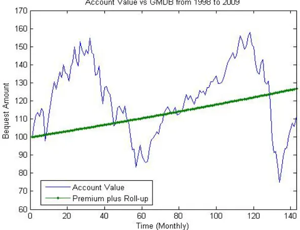
from the equity market’s downside risk. In January 1998, an individual put $100 in a VA
account and the closing date of the account was at the end of 2009. This person invested
[image:28.612.151.447.400.627.2]the entire amount in the S&P500 index.
Figure 2: Bequest Amount with roll-up benefits from 1998-2009
Figure 1 shows that if there was no GMDB option, the account value followed the index
oscillations. If the insured died at a “bad” time, the bequest amount to the beneficiary would
be low. Meanwhile, if there was a GMDB roll-up option (assume the annual roll-up rate
rp = 2%), which increased the principal 2% annually, the bequest amount to the beneficiary was protected (the downside risk was eliminated), and the account value to the beneficiary
was equal to the maximum of account value and the roll-up level (Figure 2).
2. Reset option
Here, the death benefit guarantee can be adjusted (moved up or down) at the beginning of
every reset period. The frequency of the resetting interval ranges from once a year to once
every five years. Table 3 below illustrates how the death guarantee due to the reset feature
Table 3: Computation of GMDB due to the resetting option
Dates Reset values
1/1/2005 a0
1/1/2006 max(a0, a1)
1/1/2007 max(a0, a2)
1/1/2008 max(a0, a3)
If the policyholder in the above example bought the GMDB with resetting option in
1998, the bequest amount would be described in Figure 3.
Figure 3: Bequest Amount with resetting option from 1998-2009
3. Ratchet option
This is essentially a discrete lookback option – the death benefit equals to the larger of the
amount invested or the ratcheted account value. More precisely, the death benefit guarantee
only moves up at the beginning of every ratchet period. Table 4 shows how the death
Table 4: Computation of GMDB due to the ratchet option
Dates Ratchet values
1/1/2005 a0
1/1/2006 max(a0, a1)
1/1/2007 max(a0, a1, a2)
1/1/2008 max(a0, a1, a2, a3)
If the policyholder in the above example bought the GMDB with ratchet option in 1998,
the bequest amount would be described in Figure 4.
Figure 4: Bequest Amount with monthly ratchet option from 1998-2009
The aforementioned features are provided to the policyholders with an extra premium as
riders to a base death benefit (which just contains return of the premium).
2.1
Models
purchases a variable annuity product and makes a lump sum deposit. We restrict ourselves
to insurance contracts with GMDB options only. There are two subaccounts in the VA
account. One subaccount is a fixed account, which provides a fixed interest return gt, and the other subaccount is a variable account, which provides a return related to the stock
market performance, with guaranteed minimum death benefit, i.e.
(1) kt=a0 Yt
i=1
(1 +rpi) ai−ci
ai
,
(2) bt = max(kt, at−ct) = max(kt−1(1 +rpt)
at−ct
at
, at−ct),
where at is the total account value at time t in both the fixed account (F) and the variable account (S), i.e. at =Ft+St; a0 is the initial wealth; rpt is the guaranteed rate for GMDB
at time t;kt is the guaranteed payment in the GMDB; bt is investment guaranteed amount; and a0 =b0 =k0; ct is the withdrawal at the beginning of timet, and the insured consumes
ct immediately. ct is non-negative which means that deposits are not allowed in our model.
The money in the VA account is partitioned between these two sub-accounts. dSt =
αtStdt+σtStdBt, dFt=gtFtdt, where gt is the risk-free rate and the fixed account grows at a rate gt; Bt is a standard Brownian motion. We denote byωt the percentage of wealth held in the variable subaccount and 1−ωt the proportion of wealth allocated in the fixed rate
subaccount. The amount of withdrawals isct, and it may vary with time.
(3) dat =at[ωtrt+ (1−ωt)gt]dt+ωtσtatdBt−ct,
We assume that the insureds have options to transfer money in between fixed and variable
accounts. To be more realistic, we assume 0≤ωt ≤1, which means that there are no short
sales.
We apply a constant relative risk averse (CRRA) type utility which has a functional form
U(c) =
c1−γ
1−γ, γ >0, γ 6= 1, ln(x), γ = 1.
This utility has some special properties:
• it is a homogeneous function of degree 1−γ for γ 6= 1;
• γ is the coefficient of relative risky aversion; 1/γ is the intertemporal substitution elasticity between consumption in any two periods, i.e., it measures the willingness to
substitute consumption between different periods.
If there is no possibility of death and no partial withdrawals in the accumulation stage
and in the absence of a GMDB, the individual maximizes the expected utility at retirement
date T. According to Charupat and Milevsky (2002), the objective function is
max ωt
E
1 1−γa
1−γ T
.
(4)
The solution to the objective function is equal to
ω∗ = min
r−g γσ2 ,1
,
(5)
where r is the risky asset’s expected rate of return; σ is the volatility of risky return; g is the risk free asset’s rate of return; γ is the coefficient of relative risk aversion.
During the term of the contract, there are several possible types of events: the insured
can
• transfer the funds between these two subaccounts;
• perform a partial surrender;
• completely surrender the contract;
We incorporate these events into our “without consumption” and “with consumption”
mod-els.
2.1.1 “WITHOUT CONSUMPTION” CASE
In the first step, let us assume there are no surrenders. If we only consider the insured
and beneficiary utility without consumption, we can get the objective function as
max ωt E T X t=1
βt(Yt−1
i=1φi)(1−φt)ζvB(bt) +β
T(YT
i=1φi)VT+1(aT+1)
.
(6)
The insured retires at the end of time T. φt is the survival rate at time t. ζ denotes the strength of the bequest motive and ranges from 0 to 1. If ζ = 0, the insured has no bequest motive and does not want to leave a bequest to his beneficiary; if ζ = 1, the insured has the strongest bequest motive and will treat his beneficiary like himself. vB is the beneficiary’s value function. If the insured dies before retirement, the beneficiary will get the larger of the
account value or the guaranteed amount. Once the beneficiary gets the money, the objective
function of the beneficiary is
(7) max
ωB t
E
βTB−t(YTB
i=tφi)vTB+1(bTB+1)
.
When the insured purchases the VA product, the beneficiary has TB years until retirement
age. If the insured dies at time t, the beneficiary will receive the bequest and has TB −t years until retirement age. She will optimally allocate the amount between risky and
risk-free investments, and periodically consume the amount after her retirement. However, the
beneficiary’s investment is not protected by the GMDB and we assume she has no bequest
motive. If the insured survives until his retirement age, at the end of the policy period, he
will get the entire account value without GMDB protection and annuitize it for his retirement
We get the Bellman equation for the insured:
Vt(at, bt) = (1−φt)ζvB(bt) + max
ω βφtE[Vt+1(at+1, bt+1)|at], (8)
subject to
VT+1(aT+1) =
Tmax
X
t=T+1
βt−(T+1)(Yt−1
i=T+1φi)u(¯c),
(9)
¯
c= aT+1
PTmax
t=T+1 Qt−1
i=T+1φi(1 +rf)T+1−t
,
(10)
at+1 =at(ωt(1 +rt+1) + (1−ωt)(1 +gt)), 0≤ωt≤1,
kt+1 =kt(1 +rpt), bt+1 = max(a1
Yt
i=1(1 +rpi), at+1),
= max(kt+1, at+1),
where rt is the expected risky rate of return at time t,rf is the risk free rate of return, and ¯
c is annuitization amount after retirement. In our model, the retired insured will receive a life time pay-out annuity2, and the monthly payout is ¯c. The insured consumes ¯c and gets
the utility.
2.1.2 “WITH CONSUMPTION” CASE
For simplicity, we assume that the events (the consumption and the allocation) can
only occur at a discrete time. Therefore, state variables only change at integer time points
t = 1,2,· · ·, T. The consumption, ct∈ [0, at], is taken out from the two subaccounts in the same ratio as the existing account value and are consumed immediately. We can get the
2Life time payout annuity is an insurance product that converts an accumulated investment into income
objective function as
(11)
max ωt,ct
E
T
X
t=1
βt(Yt−1
i=1φi)u(ct) +β
T(YT
i=1φi)VT+1(aT+1) +
T
X
t=1
ζβt(Yt−1
i=1φi)(1−φi)vB(bt)
.
Once the beneficiary receives the bequest bt, which is protected by the GMDB, the
objective function for the beneficiary is
(12) max ωB
t ,cBt E
TB
X
tB=t
βtB−t(YtB−1
i=t φi)u(c B t ) +β
TB−t(YTB
i=tφi)vTB+1(bTB+1)
.
The beneficiary will maximize her own utility by optimally choosing her own consumption
cB
t and investment allocation ωtB. As in the “without consumption” case, the beneficiary’s investment is not protected by the GMDB and she has no bequest motive.
The derived Bellman equation for the insured is
Vt(at, bt) = max ωt,ct
ut(ct) +βφtE[Vt+1(at+1, bt+1)|at] +ζ(1−φt)vt(bt) , (13)
subject to
VT+1(aT+1) =
Tmax
X
t=T+1
βt−(T+1)(Yt−1
i=T+1φi)u(¯c),
0≤ωt≤1, 0< ct ≤at,
at+1 = (ωt(1 +rt+1) + (1−ωt)(1 +gt))(at−ct), ¯
c= aT+1
PTmax
t=T+1 Qt−1
i=T+1φi(1 +rf)T+1
−t,
kt+1 =kt(1 +rpt)
at+1−ct+1
at+1
Following Hardy (2003), all state variables are denoted as (·)t−, (·)t+, i.e. the value
im-mediately before and after the transactions at the discrete timet, respectively. Withdrawals and consumptions occur at t−, then att+, which is still at time t but after withdrawal, the insured decides the amount to transfer between the fixed and the variable subaccounts. We
also assume that the beneficiary gets the bequest immediately at t+ just after the insured
dies at t+. Therefore, the Bellman equation will have 2 stages: at the 1st stage from t− to
t+, the insured gets the utility from consumption of withdrawal.
Vt−(at−, bt−) = max
ct
u(ct) +
Vt+(at+, bt+) ,
(14)
=⇒Vt−(at−, mt) = max
ct
u(ct) +
Vt+(at+, mt) ,
(15)
where mt=
at− bt− , at+ =at−−ct =
1− ct at−
at−,
and u(ct) +Vt+(at+, mt) =
c1t−γ
1−γ +
1− ct at−
1−γ
Vt+(at−, mt).
It is easy to see that mt is same at t− and t+. Because
bt+ =
at+
at− bt− =
1− ct at−
bt−,
mt+ =
at+
bt+
=
1− ct at−
at−
1− ct at−
bt−
= at−
bt−
=mt−.
At the second stage from t+ to (t+h)−, the insured chooses a proportion ω to invest in the
variable account,
Vt+(at+, bt) = (1−φt)ζv(max(at+, bt+)) + max
ωt
φtβhEVt+h−(at+h−, bt+h−) ,
(16)
=⇒Vt+(at+, mt) = (1−φt)ζv(max(at+, mt)) + max
ωt
φtβhEVt+h−(at+h−, mt+h−) ,
(17)
then we can get
Vt+(at+, mt) = (1−φt)ζv(max(at+, bt+)) +
(18)
+ max ωt
φtβhEVt+h−
at+((ωerh + (1−ω)egh)),
at+(ωerh+ (1−ω)egh)
bt+eph
.
2.2
Numerical Methodology
Let us first assume that the insured buys the variable annuity with GMDB options in
a lump sum at age 35. The insured can transfer and withdraw money every month. At
age 65, the insured retires and annuitizes the variable annuity to support his retirement life.
Let the expected risky rate of return r = 0.07; volatility of risky rate of return σ = 0.15; growth rate in fixed account g = 0.04; inflation rate rf = 0.03; coefficient of relative risk
aversion γ = 1.8. By Charupat and Milevsky (2002), the optimal allocation to the risky
asset is ω? = 74% at any asset level in each time period t with the survival rate φ = 1 and guaranteed rate rp = 0.
We will apply a trinomial lattice model in both “without” and “with consumption” cases.
2.2.1 “WITHOUT CONSUMPTION” CASE
Based on Hull (1997), we use a trinomial lattice to do the calculation. Assume the
move-up factor isu=eσ√3∆t; the move-down factor d= 1/u; the mean value in the variable account (S =ωa); the mean of the continuous log-normal distributionE[S] =ωaerh(assume
h= ∆t), and the variance isV ar[S] =ω2a2e2rh[eσ2h−1]; the mean value in the fixed account (F = (1−ω)a) is E[F] = (1 −ω)aegh, and variance is V ar[F] = 0; and the covariance
Cov[F, S] = 0.
According to Boyle (1988), there are three conditions to apply to the trinomial lattice:
1. the probabilities sum to one;
2. the mean of the discrete distribution is equal to the mean of the continuous log-normal
distribution;
distri-bution.
The above three conditions are,
pu+pm+pd= 1, (19)
puau+pma+pdad=a[ωerh + (1−ω)egh], (20)
pua2u2+pma2+pda2d2−(ωerh+ (1−ω)egh)2 =ω2a2e2rh[eσ
2h
−1].
(21)
By some algebraic transformation, we can get
pu =
Aω2+Bω+C
(u−1)(u−d), (22)
pd =
ω(erh−egh) +egh−1
d−1 −
Aω2 +Bω+C
(d−1)(u−d), (23)
pm = 1−
Aω2+Bω+C
(u−1)(u−d) −
ω(erh−egh) +egh−1
d−1 +
Aω2+Bω+C
(d−1)(u−d), (24)
where
A=e(2r+σ2)h−2e(r+g)h+e2gh, B = (erh−egh)(2egh−d−1), C = (egh−1)(egh−d).
Since
(25) Vt,j(ω) = (1−φ)ζv(bt,j) +βφ(puVt+1,j+1+pmVt+1,j+pdVt+1,j−1),
to maximize Vt,j, we take the first derivative on ω, and we get the optimal ω:
(26) ω? =−(d−1)BVt+1,j−Vt+1,j−1+ (u−1)(Vt+1,jVt+1,j+1)[(u−d)(e
rh−egh)−B] 2A[(d−1)(Vt+1,j−1−Vt+1,j) + (u−1)(Vt+1,j−Vt+1,j+1)]
.
We assume the insured can adjust his allocation at the beginning of each month, and
starting wealth level at time 0 is 1. The algorithm to do the numerical values can be done
as follows
1. Initialize account value at time 1: a1 = 1, and other parameter values;
2. Calculate the jump sizes u=eσ√3∆t,d= 1
u and m= 1;
3. Build the tree for account valuea by using jump sizes until age 65; 4. Set terminal value VT+1(aT+1) by using equation (9), (10);
5. For t = T to 1, at each time period, use backward induction to maximize the insured’s
utility:
5.1 Calculate the optimal allocation ω?
t by (26);
5.2 Calculate the transition probabilities pu, pd and pm by plugging ωt? into (22), (23) and (24);
5.3 Derive Vt by (25) until t = 1.
Let us first assume the base case is r = 0.07, g = 0.04, rf = 0.03, β = 0.97, rp = 0,
σ = 0.15, φ= 0.99, γ = 1.8,ζ = 0.5. Then, we will check the changes of allocation by giving some shocks: (1)r = 0.055; (2)σ = 0.25; (3) γ = 2.5; (4) ζ = 0.2; (5) p= 0.03.
Figure 5 (age 45 allocation under “without consumption” case) shows that the amount
of money allocated to the variable account at age 45 when the option is at-the-money.
An “argument” between the beneficiary and the insured is a helpful way of looking at the
results. The insured prefers the allocation determined by Merton (1969) at all times and
benefit levels. At all stock-to-strike levels, the beneficiary prefers a more aggressive allocation
than the insured, as he is protected against downside risk. This effect is most pronounced
when the account is at-the-money. When the account is significantly out-of-the-money, the
downside protection is not very valuable and the beneficiary prefers an allocation near the
Merton level. Therefore, there is no argument. When the account is significantly
in-the-money, the beneficiary does not have a strong preference as he receives the strike in (nearly)
near the at-the-money level where the beneficiary has a strong and aggressive preference.
Figure 5: Age 45 allocation under without consumption case
The effect of the argument is clearly seen in this figure by the bumps around the
at-the-money area, which are in the middle, for all parameter levels. Parameter changes primarily
affect the level of the insureds preferred allocation rather than the size of the bump.
As the risky rate of returnrdecreases from 7% to 5.5%, the variable subaccount allocation
reduces from 73% to around 37%. For r = 7%, as the asset level goes up, the allocation
increases from 73%, which is a Merton allocation, to 77% (goes up 4%) around the
at-the-money area, and then goes down to Merton allocation again; for r = 5.5%, the allocation
increases from 36.7%, to 39% (goes up 2.3%), then goes down to 36.7%. As the risky
rate of return decreases, the risky subaccount will lose some attraction to both insured and
beneficiary.
As the stock market volatility increases, i.e. σ increases from 15% to 25%, the variable
subaccount allocation reduces from 73% to around 28%. For σ = 25%, as the asset level
goes up, the allocation increases from 26.6%, which is Merton allocation, to 28.2% (goes up
allocation again. As the volatility increases, the risky subaccount will not be as attractive
as in low volatility case to both insured and beneficiary. Consistent to Merton (1969) and
Charupat and Milevsky (2002), identical Sharpe Ratios produce identical results.
As insured’s risk aversion level increases, i.e. the coefficient of relative risk aversion γ
increases from 1.8 to 2.5, the allocation at all asset levels decreases about 27%, because the more risk averse the policyholder is, the more conservative allocation decision they would
make. Asγ = 2.5, the allocation increases from 52.7% to 55% (goes up 2.3%) around at the money area.
When the roll-up rate rp increases from 0% to 3%, the bump area will move to a higher
asset level. At age 45, the highest “argument” point moves from a = 1 to 1.35, which is a significant increase. The increase of the strike price of the GMDB option is the reason for
this move.
Decreasing the bequest motive fromζ = 0.5 to 0.2 will keep the allocation level the same at almost all asset levels, but reducing the bequest motive makes insured care less about
beneficiary. The hump level around at the money area is reduced to 1.7%.
Figure 6 plots at the money allocation at all ages. It shows that at any parameter level,
as the insured gets older, he will care more about himself. As the policyholder ages, he has
less and less probability to die before retirement age. It is more likely that he, rather than his
beneficiary, will consume the assets. He will be more concerned about his post-retirement life
and keeping himself from outliving the assets during retirement. As a result, the “argument”
moves in favor of the insured, and the amount in the risky asset decreases. As the risky rate
of returnrdecreases from 7% to 5.5%, the risky account will be less attractive, as a result the insured puts less money in the risky subaccount. As the stock market volatility increases, i.e.
σ increases from 15% to 25%, a risk averse insured will take less risk by transfering money from risky subaccount to risk free account. As the insured’s risk aversion level increases,
i.e. the coefficient of relative risk aversion γ increases from 1.8 to 2.5, the insured is more concerned about the safety of the investment and will allocate less into risky subaccount.
The bequest motive ζ also has an effect, as the bequest motive decreases, the risky account allocation will slightly decrease, which also means the “argument” between the policyholder
and the beneficiary decreases at all ages. Roll-up raterp case is somewhat more complicated: Increasing the roll-up raterp increases the at the money allocation when the policyholder is at a younger age; as the insured ages, the roll-up rate becomes less and less useful to protect
the beneficiary, and as a result, the risky asset allocation drops more quickly than the base
case, and finally converges to the base case allocation. Compared with all the parameter
shocks, changes in roll-up rate rp and bequest motive ζ will only change the allocation at younger ages; as the insured ages, the allocation strategies converge. Changes in the risky
rate of returnr, coefficient of relative risk aversion or volatility of stock market cause nearly parallel shifts, which change not only at younger ages, but also at older ones.
2.2.2 “WITH CONSUMPTION” CASE
first stage, and we will get
∂Vt−(at−, mt) ∂ct
=c−tγ−
(1−γ)
1− ct at−
−γ
Vt+(at−, mt) at−
.
(27)
Let D=
1
(1−γ)Vt+(1, mt) γ1
, we can get
ct
at−
= D
1 +D.
To match the second stage, we need to modify the expression of D:
D=
1
(1−γ)Vt+(1, mt) 1γ
=
(mterpt)1−γ (1−γ)Vt+(mterpt, mt)
γ1
.
At the second stage, immediately after the consumption, the insured may be dead and
the insurer will pay the GMDB amount to the beneficiary at t+. If the insured still survives,
he will choose allocation to the separate subaccounts. This will be the same procedure as in
the “without consumption” case.
Table 5: Common Parameters in the Base case
Strength of Bequest Motive ζ 0.5
Subjective Discount Rate β 0.97
Risk Free Rate rf 3%
Coefficient of Relative Risk Aversion γ 2
Growth Rate of Fixed Subaccount rg 4%
Expected Return of Risky Asset r 7%
Volatility of Risky Return σ 15%
GMDB roll-up rate rp 0
Annual Survival Rate φ 0.99
With the partial withdrawal option, one will see the behavior of the insureds change from
the previous case. To do the sensitivity tests, the values of base parameters are set as in
table 5.
a. Risk Aversion Sensitivity
Figure 7: At the Money Allocation with differentγ under consumption case
The purpose of this sensitivity test is to discover the optimal choices for the policyholder
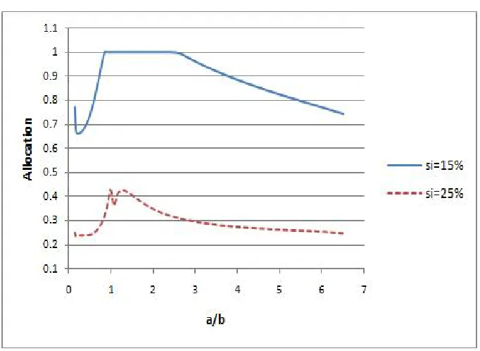
if all but one coefficient, relative risk aversion (γ), were kept constant. Figure 7 shows that as the risk aversion level increases, the policyholder will less likely to invest money into the
variable subaccount. For all γ > 1, the proportion in the variable subaccount will decrease as the insureds age. Asγ increases, the proportion in the variable subaccount will decrease. All of these are consistent as in the “without consumption” case. Asγ <1, since the insured is not very risk averse, he will put all the money into his variable subaccount.
Figure 8 shows that the pre-retirement consumption ratio changes for different levels of
increase, because people will be increasingly concerned about the investment risk in the
future. A bird in the hand is worth two in the bush, so they will prefer consuming now
rather than investing for the future. Also as the insured ages, he will more strongly consider
for himself than his beneficiary. As in the “without consumption” case, the “argument”
moves in favor of the insured. Therefore, the consumption ratios increase under different
risk aversion levels. One can also find that the consumption ratios converge under different
risk aversion levels at Merton level once the policyholder reaches his retirement age.
Figure 8: At the Money Withdrawal ratio with differentγunder consumption case
Figure 9 shows, at age 45,the proportion of consumption to account value will correspond
given different levels of risk aversion. The proportion of funds consumed is roughly constant
when the GMDB is in the far out-of-the-money area, and the value of the consumption
proportion is consistent with the value derived in the Merton model. Asγ <1, consumption
ratio decreases as the GMDB becomes more deeply in the money; while as γ > 1, , the
consumption level increases as the asset level decreses (GMDB goes deeper and deeper
far more than the insured by roll-up property and even a mild bequest motive will cause the
insured to maintain the account.
Figure 9: Age 45 proportion of consumption with differentγunder consumption case
The reason for the counterintuitiveγ >1 result in figure 9 is that we assume withdrawals from the variable annuity are the only source of consumption. For most currently available
variable annuities, the GMDB strike is reduced proportionally with the reduction of the VA
account value. When γ = 1, utility is logarithmic. A proportional reduction in the higher
strike value reduces the beneficiary’s utility by exactly the same amount as a reduction of
the lower account value harms the insured’s utility. When γ <1, the beneficiary’s utility is reduced by more than the insureds utility. When γ >1, the beneficiary’s utility is actually reduced less than the insured’s utility is. In the most extreme case, the insured’s utility
can approach −∞. The insured sells his beneficiary up the river for a loaf of bread. A
more realistic model would include an outside consumption source in addition to the partial
withdrawals from the variable annuity account. This has been done in the next section.
levels. If the insured is less risk averse (γ <1 or around 1), he will put the entire fund in the variable subaccount. At γ >1, if the account value is small and less than the at-the-money level, the beneficiary does not care about the allocation because she has downside protection,
and the insured still allocates the wealth using Merton’s method. If the account value is
greater than the guaranteed value, the beneficiary and the insured agree on the allocation.
But around at-the-money area, there are arguments between them, bequest motive will take
effect and more money will be put in the risky account. As the risk aversion gets larger, the
insureds will care more for themselves. Therefore, the bump level decreases as risk aversion
level increases.
Figure 10: Age 45 allocation with differentγ under consumption case
b. Bequest Motive Sensitivity
The purpose of this sensitivity test was to discover the optimal choices for the policyholder
if all but one parameter, bequest motive (ζ), were kept constant. Figure 11 shows the
at-the-money asset allocation for different bequest motives with γ = 2. When the bequest motive
motive increases, the proportion in the risky account will increase. But at any non-zero level
of policyholder’s bequest motive, the allocation to the risky account decreases as age grows
until converges to the allocation at ζ = 0 (the Merton’s allocation) at age 65.
Figure 11: At the Money Allocation with differentζ under consumption case
As the bequest motive level ζ increases, the pre-retirement consumption ratio in each
period will decrease as shown in figure 12. With a larger bequest motive, the insured prefers
to reduce the consumption to leave more money to his beneficiary. The consumption (partial
withdrawal) will increase as the insured ages under all bequest motive levels. One can see
that the higher the bequest motive is, the lower the consumption ratio is. The insured
cares more for himself as he grows older. One can also observe that the consumption levels
converge as the insured grows older and consumption ratios become the same at retirement
age. The reason is that after the insured retires, the wealth in VA account will become a
Figure 12: At the Money Withdrawal ratio with differentζ under consumption case
Figure 13 shows the consumption ratio vs. account value at age 45 with different levels
of bequest motive. As the bequest motive increases, the proportion of funds consumed will
decrease. As the GMDB goes deeper in-the-money, the consumption ratios at all non-zero
bequest motives converge to the zero bequest level. In addition, consumption ratios stay
constant as the GMDB goes out-of-the-money. This is also counter-intuitive, and the reason
is the same as in the risk aversion sensitivity test: we assume that withdrawals from the
variable annuity are the only source of the policyholder’s consumption. In this test, we set
γ = 2 in theζ test, the beneficiary’s utility is actually reduced less than the insured’s utility is, so the insured becomes selfish. The problem should disappear if an outside income is
Figure 13: Age 45 proportion of consumption with differentζ under consumption case
Figure 14: Age 45 allocation with differentζ under consumption case
with different bequest motives. As ζ = 0, the insured has no bequest motive and he only cares about himself, and his allocation decision follows the Merton rule. As the insured
has the bequest motive and wants to leave a bequest to his beneficiary, he starts to make
choices to maximize the joint utility. Therefore, around the at-the-money area, the insured
breaks the Merton’s rule and tries to take more risk to help the beneficiary accumulate more
benefits. One can observe the spikes around at-the-money area corresponding to different
levels of bequest motive: the stronger the bequest motive is, the higher the spike (risky
allocation) is.
c. Roll-up Rate Sensitivity
Figure 15: At the Money Allocation with differentrp under consumption case whenγ= 2
The purpose of the roll-up rate sensitivity test was to discover the optimal choices for the
policyholder if only one variable, roll-up rate, was changed. Figure 15 shows at-the-money
asset allocations under different roll-up rates. At any level of roll-up rate, the insured reduces
(age 35 to 65), which is consistent to the “without consumption” case. As the insured ages,
the insured has more probability to get the wealth himself. Therefore, he will care more
about his retirement life and put more money into riskless account. As the insured is young
(at the beginning of the contract), higher roll-up raterp encourage more risky allocation. As the insured ages, roll-up protection weakens, because the beneficiary has less chance to get
the GMDB protection.
Figure 15 is somewhat counter-intuitive: At 45 years old, the risky allocation forrp = 0% is highest one, although therp = 0% case provides least downside protection. This is because for rp = 1% and rp = 3%, the level of return of premium and roll-up benefits is increasing period by period. Therefore a = 1 is not a real “at-the-money” area for rp > 0, and the argument area forrp >0 will go higher as the insured ages, but as usual the hump level will decrease.
Figure 16: At the Money proportion of consumption with differentrp under consumption case whenγ= 2
Figure 16 (at-the-money consumption ratios under different roll-up rates withγ = 2) and