Copula based downscaling of spatial rainfall: a proof of concept

www.hydrol-earth-syst-sci.net/15/1445/2011/ doi:10.5194/hess-15-1445-2011

© Author(s) 2011. CC Attribution 3.0 License.

Earth System

Sciences

Copula-based downscaling of spatial rainfall: a proof of concept

M. J. van den Berg1, S. Vandenberghe1, B. De Baets2, and N. E. C. Verhoest1

1_{Laboratory of Hydrology and Water Management, Ghent University, Coupure links 653, 9000 Ghent, Belgium} 2_{Department of Applied Mathematics, Biometrics and Process Control, Ghent University, Coupure links 653,} 9000 Ghent, Belgium

Received: 23 December 2010 – Published in Hydrol. Earth Syst. Sci. Discuss.: 13 January 2011 Revised: 18 April 2011 – Accepted: 2 May 2011 – Published: 11 May 2011

Abstract. Fine-scale rainfall data is important for many

hy-drological applications. However, often the only data avail-able is at a coarse scale. To bridge this gap in resolution, stochastic disaggregation methods can be used. Such meth-ods generally assume that the distribution of the field is sta-tionary, i.e. the distribution for the entire (fine-scale) field is the same as the distribution of a smaller region within the field. This assumption is generally incorrect and we provide a proof of concept of a method to estimate the distribution of a smaller region. In this method, a copula is used to con-struct a bivariate distribution describing the relation between the scales. This distribution is then used to estimate the dis-tribution of the fine-scale rainfall within a single coarse-scale pixel, by conditioning on the coarse-scale rainfall depth.

1 Introduction

Hydrological models are used in a variety of small-scale applications, including flood forecasting (Winchell et al., 1998), water management (Varis et al., 2004), and land slide risk assessment (Collison et al., 2000). These models often simulate hydrological processes and water fluxes at a small scale (<100 km2), requiring rainfall data with a high spatio-temporal resolution. However, such data is not available for many parts of the world as rain-gage networks are lacking in coverage and General Circulation Models (GCMs) and re-mote sensing cannot provide data at the required resolution (Onof et al., 1998; Deidda, 2000). This lack in resolution re-sults in a scale gap where observations are only available at a coarser scale, but not at the required finer scale.

Correspondence to: M. J. van den Berg ([email protected])

The scale gap between the observed data and the hydrolog-ical model can be mitigated using stochastic methods. This is done by investigating the coarse-scale rainfall from which parameters for a suitable synthetic rainfall model are derived. A first approach consists of representing rainfall as a stochas-tic process of cluster-based rectangular pulses, and found its origin in the mathematical description of rainfall, starting with a seminal paper by Le Cam (1961). This has led to the development of rainfall models based on Neyman-Scott and Bartlett-Lewis point processes (Onof et al., 2000). These models, which recently have been expanded into the spatial domain (e.g. Cowpertwait et al., 2002; Burton et al., 2008), use parameters that have a physical interpretation, such as the mean intensity and the mean duration of a raincell (Onof et al., 2000).

A second approach to bridge the scale gap between ob-served rainfall and the hydrological model applies cascade models. In contrast to the Neymann-Scott and Bartlett-Lewis models, cascade models do not use physically-based vari-ables, but rather a physically relevant model structure: the (multiplicative) cascade. These models are derived from sta-tistical fractals (Lovejoy and Mandelbrot, 1985) and con-stitute the first spatial synthetic rainfall models (Schertzer and Lovejoy, 1987). Further model development (Deidda et al., 1999) resulted in spatio-temporal synthetic rainfall models. One advantage of these models over the Neyman-Scott and Bartlett-Lewis models is that the resulting cascade-based synthetic data better represent the spatial structure of rainfall, which may prove important in small-scale applica-tions (Willems, 2001).

14462 van den Berg et al.: Copula-based downscaling of spatial rainfallvan den Berg et al.: Copula-based downscaling of spatial rainfall

(a) (b)

Fig. 1: A coarse-scale image of the rainfall depth (mm) (a), and its corresponding sub-pixel standard deviation (b).

toregressive model is used to generate a random field which is passed through a non-linear filter to obtain a rainfall field that has similar spatial patterns as the large-scale rainfall field. For a more elaborate introduction to the various meth-ods of simulating rainfall, we refer to Onof et al. (2000), and Ferraris et al. (2002).

Many different downscaling methods exist, however, the above three categories give a brief summary of the most common methods. All these methods can be used to down-scale a rainfall field, however, forcing the model to some observed coarse-scale data has proven to be difficult. Gen-erally, only the last group of methods offers a way to take into account other assumptions and forcing data (Mackay et al., 2001; Rebora et al., 2006). Here, the specific point of interest is the use of small-scale sub-pixel distributions to force the fine-scale field to follow the coarse-scale field. For example, Mackay et al. (2001) use a Gamma distribu-tion for subgrid variability, and Rebora et al. (2006) use a single log-normal distribution across the entire field. How-ever, a cursory glance at a rainfall field shows that it is likely that the local variability is not stationary throughout the field, and that it varies with the depth of the coarse-scale field (see Fig. 1). In this paper, we present a method to estimate the subgrid variability distribution function needed in the down-scaling of coarse-scale rainfall. Therefore, a novel method is explored that describes the dependence between the coarse-and the fine-scale rainfall depth using a copula. Furthermore, it allows for modeling the sub-pixel probability distribution within one coarse-scale pixel.

This paper is structured as follows. The data used for empirical testing is introduced first. Section 3 presents the framework of the copula-based methodology, and Sect. 4 in-troduces some basics on copulas. Subsequently, the frame-work is tested and validated in Sect. 5. Finally, the results are discussed and conclusions are drawn.

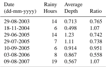
Table 1: The seven events for which data was available, to-gether with the number of rainy hours on that day, the aver-age depth (mm) for all active pixels. The ratio expresses the proportion of dry to wet pixels within the radar image.

Date Rainy Average

(dd-mm-yyyy) Hours Depth Ratio

29-08-2003 14 0.713 0.765

18-11-2004 6 0.498 1.07

29-06-2005 14 1.23 0.742

29-07-2005 7 1.11 0.738

10-09-2005 6 0.914 0.951

03-08-2006 8 0.867 0.558

09-08-2007 19 0.567 1.07

2 Data

The data for this study were acquired by a weather radar near Wideumont, Belgium, operated by the Belgian Royal Mete-orological Institute (RMI). The installation covers a circular area with a radius of 240 km, producing a scan every 5 min. The region covered includes coastal landscapes to the west, and a low mountain range, the Ardennes, to the east with land cover mostly composed of forests, urbanization and agri-culture. The entire region has a temperate climate and re-ceives about 800 mm of rain annually, almost uniformly dis-tributed throughout the year (De Jongh et al., 2006) and a mean monthly temperature which varies between 18◦C in June and 3◦C in January.

The dates, at which radar imagery is available, are selected based on rain-gage readings from a network across Belgium, where the rainfall was required to have a minimum Peak-over-Threshold return period of 10 yr to be included in the dataset. This resulted in a dataset consisting of the days listed in Table 1. For these days, the number of rainy hours has been listed, along with the average intensity for each rain-storm, and the ratio of dry pixels to wet pixels. Images that did not display rainfall were removed from the dataset as they hold no information.

The raw radar data are stored as digital numbers, repre-senting reflectivities ranging from −31.5 dB to 95.5 dB in steps of 0.5 dB. Because of the 0.5 dB step, conversion of these reflectivities into rainfall rates results in discrete rain-fall intensity values. Such data is likely to result in repeated values (often referred to as ties) which can lead to prob-lems later on in the analysis. Similar to Vandenberghe et al. (2010b), uniform random noise ranging from−0.25 dB to 0.25 dB is introduced to perturb the data and to overcome the problem of ties. This perturbed data is then converted into rainfall intensities using the Marshall-Palmer

relation-Hydrol. Earth Syst. Sci., 15, 1–13, 2011 www.hydrol-earth-syst-sci.net/15/1/2011/

Fig. 1. A coarse-scale image of the rainfall depth (mm) (a), and its corresponding sub-pixel standard deviation (b).

include Markov Random Fields (Mackay et al., 2001; All-croft and Glasbey, 2003), filtered autoregressive processes, and the superimposing of random fields (Ferraris et al., 2003a). Examples of the application of these methods in-clude Rebora et al. (2006) and Pegram and Clothier (2001) where an autoregressive model is used to generate a random field which is passed through a non-linear filter to obtain a rainfall field that has similar spatial patterns as the large-scale rainfall field. For a more elaborate introduction to the various methods of simulating rainfall, we refer to Onof et al. (2000), and Ferraris et al. (2003a).

Many different downscaling methods exist, however, the above three categories give a brief summary of the most common methods. All these methods can be used to down-scale a rainfall field, however, forcing the model to some observed coarse-scale data has proven to be difficult. Gen-erally, only the last group of methods offers a way to take into account other assumptions and forcing data (Mackay et al., 2001; Rebora et al., 2006). Here, the specific point of interest is the use of small-scale sub-pixel distributions to force the fine-scale field to follow the coarse-scale field. For example, Mackay et al. (2001) use a Gamma distribu-tion for subgrid variability, and Rebora et al. (2006) use a single log-normal distribution across the entire field. How-ever, a cursory glance at a rainfall field shows that it is likely that the local variability is not stationary throughout the field, and that it varies with the depth of the coarse-scale field (see Fig. 1). In this paper, we present a method to estimate the subgrid variability distribution function needed in the down-scaling of coarse-scale rainfall. Therefore, a novel method is explored that describes the dependence between the coarse-and the fine-scale rainfall depth using a copula. Furthermore, it allows for modeling the sub-pixel probability distribution within one coarse-scale pixel.

This paper is structured as follows. The data used for empirical testing is introduced first. Section 3 presents the framework of the copula-based methodology, and Sect. 4 in-troduces some basics on copulas. Subsequently, the

frame-Table 1. The seven events for which data was available, together with the number of rainy hours on that day, the average depth (mm) for all active pixels. The ratio expresses the proportion of dry to wet pixels within the radar image.

Date Rainy Average

(dd-mm-yyyy) Hours Depth Ratio

29-08-2003 14 0.713 0.765

18-11-2004 6 0.498 1.07

29-06-2005 14 1.23 0.742

29-07-2005 7 1.11 0.738

10-09-2005 6 0.914 0.951

03-08-2006 8 0.867 0.558

09-08-2007 19 0.567 1.07

work is tested and validated in Sect. 5. Finally, the results are discussed and conclusions are drawn.

2 Data

The data for this study were acquired by a weather radar near Wideumont, Belgium, operated by the Belgian Royal Mete-orological Institute (RMI). The installation covers a circular area with a radius of 240 km, producing a scan every 5 min. The region covered includes coastal landscapes to the west, and a low mountain range, the Ardennes, to the east with land cover mostly composed of forests, urbanization and agri-culture. The entire region has a temperate climate and re-ceives about 800 mm of rain annually, almost uniformly dis-tributed throughout the year (De Jongh et al., 2006) and a mean monthly temperature which varies between 18◦C in June and 3◦C in January.

The dates, at which radar imagery is available, are selected based on rain-gage readings from a network across Belgium, where the rainfall was required to have a minimum Peak-over-Threshold return period of 10 yr to be included in the dataset. This resulted in a dataset consisting of the days listed in Table 1. For these days, the number of rainy hours has been listed, along with the average intensity for each rain-storm, and the ratio of dry pixels to wet pixels. Images that did not display rainfall were removed from the dataset as they hold no information.

The raw radar data are stored as digital numbers, repre-senting reflectivities ranging from −31.5 dB to 95.5 dB in steps of 0.5 dB. Because of the 0.5 dB step, conversion of these reflectivities into rainfall rates results in discrete rain-fall intensity values. Such data is likely to result in repeated values (often referred to as ties) which can lead to prob-lems later on in the analysis. Similar to Vandenberghe et al. (2010b), uniform random noise ranging from −0.25 dB to 0.25 dB is introduced to perturb the data and to overcome the problem of ties. This perturbed data is then converted

into rainfall intensities using the Marshall-Palmer relation-ship (Marshall and Palmer, 1948)

R= b

s

100.1·ZdB

a , (1)

whereZdBis the reflectivity[dB]andaandbare dimension-less parameters, respectively equal to 200 and 1.6 as sug-gested by Heylen and Maenhout (1994). This results in a set of spatially distributed rainfall intensities, each represent-ing a surface over which the estimate is valid. However, the resolution of the image is not constant but changes with dis-tance from the radar station (Heylen and Maenhout, 1994). As this is likely to influence the analysis, the data has been re-sampled to a grid of square pixels of 600 m×600 m and the 12 images within one hour are summed to form the total depth for a single hour.

The processed data was artificially downgraded to obtain the coarse-scale images with a pixel size of 19.2 km×19.2 km. Each coarse-scale pixel is obtained by spatially averaging over the rainfall depths of the 1024 fine-scale pixels (hereafter referred to as sub-pixels) covered by a single coarse-scale pixel (Ferraris et al., 2003a; Deidda, 2000). Thus, the relation between the coarse scale fieldDλ

and the fine scale fieldD_λ0, can be expressed as

Dλ(i,j )=

1 n2

in X

k=(i−1)n+1 j n X

l=(j−1)n+1

Dλ0(k,l), (2)

whereiandj are location indices at the coarse scale,kand l denote the location at the finer scale andnis the number of rows (and columns) of sub-pixels within one coarse-scale pixel.

3 Framework

Downscaling of rainfall fields at the image scale, as it is gen-erally done in literature, does not specify a local cumulative distribution function (CDF) for the sub-pixels belonging to a coarse-scale pixel. It does not model the local fluctuations in the fine-scale distribution of the entire field. However, one can expect that the distribution of the local fine-scale rain-fall, e.g. within a single coarse-scale pixel, will vary across the entire rainfall field. These local distributions may deviate (strongly) from the total field fine-scale distribution, and it can be expected that the shape of these distributions will de-pend on the corresponding coarse-scale observation, among other factors, as can be concluded from Fig. 1. When the coarse-scale rainfall depth is shown together with the corre-sponding sub-pixel standard deviation field, the relation be-tween the distribution and the coarse-scale depth becomes evident. Therefore, to model these varying sub-pixel proba-bility density functions, one should account for the observed

rainfall depth in the coarse-scale pixel by considering the de-pendence between the observed coarse-scale depth and the corresponding fine-scale sub-pixels.

In this paper, a framework is introduced which allows for the derivation of the modeled cumulative distribution func-tion of the sub-pixel rainfall depth at a small scale, given a coarse-scale rainfall depth; this framework is depicted in Fig. 2. Paramount in this framework is the use of a copula to model the dependence between the coarse- and fine-scale rainfall depths given their marginal distribution functions.

Within the framework, the coarse-scale distribution func-tion is first fitted to the entire rainfall image (Fig. 2e). The field-wide fine-scale cumulative distribution function (Fig. 2c) is then derived from the coarse-scale cumulative distribution function through scaling laws. Further, the de-pendence between the coarse- and fine-scale variables can then be described by means of a copula C (Fig. 2d):

Fλ0_λ(d_λ0,d_λ)=C(F_λ0(d_λ0),F_λ(d_λ))=C(u,v), (3) which is obtained through fitting to a set of corresponding coarse- and fine-scale wet pixels. Note that the upper case Dhas been replaced by the lower cased to denote the use of a single pixel; also, in this context the spatial organiza-tion of the field is disregarded and thus they are referred to as variables. C is a copula, a bivariate distribution function on the unit square with uniform marginals (see Sect. 4). A copula, together with the coarse- and fine-scale marginal dis-tribution functions and their inverses, can describe the joint probability distribution. The validity of this approach is as-sured by Sklar’s theorem (see Nelsen, 2006), which states that for every bivariate distribution with continuous marginal distributions, there exists a unique copula.

The modeled sub-pixel distribution of a wet coarse-scale pixel with observed depthdmcan be calculated from the joint probability distribution. To do this, the copula is conditioned to the valuevm=Fλ(dm), leading to the conditional cumula-tive distribution function (Fig. 2a), calculated as:

FU|V(u|vm)=P(U≤u|V=vm)=

∂C(u,v) ∂v

_v=v

m

. (4)

In this equationUandV correspond to the cumulative prob-abilities ofDλ0 andD_λ, i.e. the depth at the coarse and fine scale. Then using the fine-scale marginal distribution,Ucan be transformed into its fine-scale rainfall depthDλ0 (Fig. 2c) (e.g., x0=F_λ−01(u0)). This is possible by virtue of Eq. (3) which shows that corresponding values ofU andDλ0 have the same probability of occurrence, i.e.

1448 van den Berg et al.: Copula-based downscaling of spatial rainfall

Fig. 2. A graphical representation of the framework used to retrieve the sub-pixel distribution. In the lower left, the copula is depicted, and in the top left, a slice of the copula representingP (U≤u,V≤v). Starting at the coarse-scale distribution, one obtains the probability (rank) of the value used for conditioning. This value is used in the copula to find the conditional probability of the fine-scale ranks, which are then ’projected’ using the fine-scale distribution to find the conditional probability of the sub-pixel rainfall depths.

The cumulative distribution function _P(U≤u|V =vm) only represents the wet regions of the rainfall field. To extend this to the entire rainfall field within a coarse-scale pixel, in-cluding the intermittency, the fraction of dry fine-scale pixels should be accounted for. This fraction is modeled using an exponential function

f (v)=eav, (6)

which was fitted to several coarse-scale pixels. In Fig. 4 the relation between the fraction of dry pixels and the coarse-scale rainfall depth is depicted, as well as the fit of Eq. (6). Note that this function is not probabilistic in nature, but de-scribes the relationship between the fraction of dry pixels P (X=0)and the coarse-scale value. Finally, the sub-pixel

distribution, including zero-valued pixels, is found as F_U+_|V(u|vm)=f (vm)H (u)+(1−f (vm))FU|V(u|vm), (7) whereH (u)is the Heaviside function which is equal to one for allu≥0 and zero elsewhere.

4 Copulas

Copulas have gained increased attention in hydrological studies, including investigations into rainfall (Serinaldi, 2009; De Michele and Salvadori, 2003; Vandenberghe et al., 2010b; Grimaldi and Serinaldi, 2006), storm generators (Kao and Govindaraju, 2008; Salvadori and De Michele, 2006; Vandenberghe et al., 2010a) and data assimilation (Gao et al.,

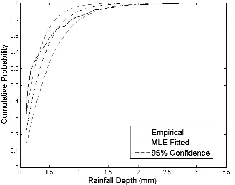
Fig. 3. The coarse-scale empirical marginal distribution and the fitted coarse-scale marginal distribution.

2007). This increased popularity can be attributed to the flex-ibility copulas offer for describing multivariate dependence (Genest and Favre, 2007).

The increased tractability offered by the use of copulas is due to the fact that the fitting of a bivariate distribution function is split into two more manageable problems, the marginal distribution functions on the one hand, and the de-pendence between them on the other hand. To illustrate this, a simple example in the context of this paper is pre-sented. For more mathematical details, the reader is referred to Nelsen (2006), Genest and Favre (2007) and Salvadori and De Michele (2007).

Consider two scale levels, a fine-scale level and a coarse-scale level, respectively with resolutionsλ0 and λ, both of the same rainfall field. These fields are represented as cou-ples(dλ,dλ0), where a single coarse-scale pixeld_λcan have several corresponding fine-scale pixelsdλ0, i.e. each coarse scale pixel leads toNcouples whereNis the number of fine-scale pixels within the coarse-fine-scale pixel. Assume that both scale levels are observable and that their rainfall depths are described by cumulative distribution functionsFλ andFλ0. These marginal distribution functions map the random vari-ables to the unit intervalI, according to:

(

u=Fλ0(d_λ0)

v=Fλ(dλ)

⇐⇒

( dλ=F

[−1]

λ0 (u) dλ0=F[−1]

λ (v)

, (8)

whered denotes a single pixel from the fieldD, anduand vare single pixels from the probability-transformed fieldsU andV.F_λ[−1]denotes the pseudo-inverse, which corresponds to the inverse if it is defined everywhere on R. Since the

transformed fieldsU andV are both uniformly distributed,

Fig. 4. The fraction of zero rainfall cells at fine scale compared to the coarse-scale value.

their pixelsuandvcan be approximated according to:

u=

Pn j=1I(d

j λ0< dλ0)

n , (9)

v=

Pn j=1I(d

j λ< dλ)

n ,

for all pixelsdinD, where I()is the indicator function (Gen-est and Favre, 2007). The superscriptj is an index number identifying the pixels within a field.

The bivariate copula of the transformed variablesu,vis a function C:_I×_I→_I, i.e. it maps values from the unit square

I×Ito the unit intervalI. Moreover, it satisfies the following

conditions:

– for allu,v∈_I

C(u,0)=0,C(0,v)=0,C(u,1)=u,C(1,v)=v . (10)

– for allu1,u2,v1,v2∈Ifor whichu1≤u2andv1≤v2

C(u2,v2)−C(u2,v1)−C(u1,v2)+C(u1,v1)≥0. (11) These conditions imply that C is an increasing function. The link between bivariate copulas and bivariate distribution functions is expressed by the theorem of Sklar (see Nelsen, 2006) as given in Eq. (3). This theorem states that a bivariate copula results in the same probability as the multivariate dis-tribution function, however it is calculated from the uniform marginal distribution functions of the variablesUandV.

1450 van den Berg et al.: Copula-based downscaling of spatial rainfall parameter free. Furthermore, the copula is invariant under

strictly increasing transformations of the marginals and the bivariate distribution function is no longer dependent on the marginals allowing any (continuous) distribution functions to be joined with the copula. In this paper, the coarse- and fine-scale marginals are coupled to form a joint distribution function using the dependence model provided by a copula. A large number of different copulas exist, covering a wide range of different behaviors. For example, the tail behavior is difficult to capture using data and often described by means of a parametrical copula. Also, more common copulas ex-ist such as the Gaussian copula which, when combined with Gaussian marginals, describes the bivariate Gaussian joint probability distribution function.

However, fitting a parametrical copula has proven to be non-trivial, and research is still ongoing (Sch¨olzel and Friderichs, 2008). Because of this, an empirical, non-parametrical copula provides an appealing parsimony, and retains all information found in the data as well. Therefore, we opted to work with the empirical copula, although future research will investigate the use of parametrical copulas in the proposed framework. The function C can be empirically represented by the joint rank of the couples(ui,vi), given by

Cn(u,v)=

1 n

n X

i=1

I(ui≤u,vi≤v). (12)

This equation calculates the cumulative probability of each point in the dataset, representing the theoretical copula C as a set of empirical points Cn(u,v).

5 Results

In this section, the application of the framework is discussed and validated. First, the scaling laws and the empirical cop-ula will be shown to be effective for modeling the relations observed in the data. Then, several practical issues that were observed will be explained.

5.1 Assessment of the scaling laws

The distribution of spatial rainfall fields is often represented by means of a Gamma distribution (Wilks, 1999; Vrac and Naveau, 2007; Mackay et al., 2001). This distribution is also used in this study and exhibits a good fit (see Fig. 3). More-over, if the rainfall depth follows the Gamma distribution at coarse scaleλand shows simple scaling, or fractal behavior (Gupta and Waymire, 1990), then the distribution at the fine scaleλ0is known as well. This relation will be used to down-scale the field-wide distribution in this study and is defined as

t·0(k,θλ)=0(k,t·θλ). (13)

0(k,θλ)denotes the Gamma distribution with shape

param-eterkand scale parameterθλ. t is a variable factor that

de-scribes the relation between scale levelsλandλ0. Further-more, whilekis constant over all scales, the scale parameter changes with each scale such thatθλ0=t·θ_λ. As mentioned before, the scaling of the Gamma distribution is tied to frac-tal behavior (Gupta and Waymire, 1990). Therefore, in order to findt, the fractal scaling laws need to be examined (see Veneziano et al., 2006; Gupta and Waymire, 1990; Menabde et al., 1999).

Consider the coarse-scale rainfall fieldDλwhose scaling

behavior is fractal (Veneziano et al., 2006; Ferraris et al., 2003b). Then, the scaling behavior of this field can be de-scribed as (Veneziano et al., 2006)

Dλ d

=r−HDrλ. (14)

H is a constant over all scales, the scaling factorr=λ0/λ and=d denotes equality in distribution. SinceDλ=d0(k,θλ),

Eq. (14) becomes rH0(k,θλ)

d

=0(k,θλ0), (15)

and thust=rH. The value ofHcan be found by computing the expected value on both sides of Eq. (15):

rHE[0(k,θλ)]=E[0(k,θλ0)], (16) whereE[·] denotes the expectation of the distribution. By log transforming Eq. (16), one obtains:

H·log₁₀(r)=log₁₀

_E[0(k,θ λ0)] E[0(k,θλ)]

. (17)

Hence, H can be found as the slope of the linear fit to this relation. This relation has been fitted to a series of ten randomly selected images, and the results are shown in Fig. 5. The fitted line shows a good consistency with the re-sults, and the resultingH≈ −0.10 has been used throughout this study; this value is consistent with results obtained by Gupta and Waymire (1990). Summarizing, the marginal dis-tribution of the coarse-scale image is determined by fitting a Gamma distribution to the empirical CDF. From this coarse-scale image, the fine-coarse-scale CDF is determined by applying Eq. (15) withH= −0.10.

5.2 Construction of the empirical copula

Once the marginal distributions of the rain fields on both scales are obtained, the dependence structure between the coarse-scale pixels and their corresponding sub-pixels needs to be determined. Since this paper is considered a proof of concept, an empirical copula will be used to describe the dependence, as a parametrical copula may introduce errors due to an improper representation of the actual dependence. However, the empirical copula, if it is to represent the depen-dence properly, should be constructed from carefully chosen

Fig. 5. Regression analysis between log₁₀(r) and log₁₀(µλ0

µλ),

whereµλ=E[0(k,θλ)] .

data. Moreover, issues such as not representing every possi-ble point in the domain and noise need to be taken into ac-count. In the following paragraphs, the practical application and implementation of the empirical copula in our frame-work will be outlined.

The marginal distributions, as well as the copula itself, need to be continuous. However, rainfall cannot be fully de-scribed by a single, continuous distribution because of the intermittency (Onof et al., 1998), which causes a singularity at zero rainfall in the probability distribution function. There-fore, rainfall is often described as a discrete (binomial) distri-bution that determines whether or not it is raining in a pixel, and a distribution to determine the rainfall depth of the wet pixels. Hence, a copula cannot be fitted directly to a rain-fall field if it contains pixels without rainrain-fall, i.e. dry pixels. To cope with this, all dry pixels were removed from the data used, making the copula only applicable to rainfall in a wet pixel both on the coarse and the fine scale.

In Sect. 3, a framework for deriving the sub-pixel distri-bution was described which requires that the copula is con-tinuous. However, this condition is not necessarily fulfilled when using an empirical copula. For example, the deriva-tive in Eq. (4) cannot be directly assessed from the empiri-cal copula because it consists of points instead of a continu-ous surface. This issue is solved by linearly interpolating the available points to estimate the cumulative probability of a point wherever no empirical value is available. However, as in any empirical approach, if insufficient data are available, noisy and inaccurate results are obtained. This is especially an issue near the upper edge of the copula domain.

For each coarse-scale pixel the cumulative probability vm=0λ(dm)is estimated from a fitted Gamma distribution. This value is then used to derive the conditional probability

distribution function using Eq. (7). However, as an empirical copula is used, the derivative in this equation is approximated as:

FU|V(u,vm)≈

C(u,vm+δ)−C(u,vm)

δ , (18)

requiring that two slices need to be extracted from the cop-ula, i.e. C(u,vm+δ)and C(u,vm), for which, when needed, linear interpolation on the empirical copula is performed. Fi-nally, the obtained CDF is rescaled to the fine-scale domain through the application of the inverse Gamma distribution of the fine-scale rainfall field resulting in the modeled fine scale distribution of the non-zero rainfall sub-pixels.

In order to test the framework, an empirical copula needs to be used which preserves the scale dependencies valid for the storm at hand. However, constructing these copulas from an analysis of the coarse- and fine-scale pixels within the image for which the sub-pixel distribution functions are to be derived may introduce false optimism. We therefore de-rived an empirical copula for the rainfall field of the same storm as observed 5 h prior to the image to be downscaled; this approach is followed unless mentioned otherwise. For this time frame, it is assumed that the scaling dependencies remain similar, but that the actual rainfall field has already evolved sufficiently to prevent over-fitting on a specific im-age. The validity of this approach will be further investigated in Sect. 5.4.4.

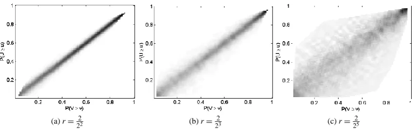
The copulas obtained from various images show a con-sistent behavior in time and between different scales, see e.g. Fig. 6, and some common patterns are observed. These patterns are easily explained as an effect of the changing scale difference and the numerical properties of scaling, al-though they are not the result of the data treatment itself.

5.3 Construction of the intermittence model

14528 van den Berg et al.: Copula-based downscaling of spatial rainfallvan den Berg et al.: Copula-based downscaling of spatial rainfall

(a)r= 2

22 (b)r=₂23 (c)r=₂25

Fig. 6: Three copula densities, constructed from the same image, but using different scale stepsr.

(a) (b)

Fig. 7: An illustration of the EMD. The difference between the functions is shown as mass bars. These bars, or parts of them, need to be moved around in such a way that the dark gray bars (surplus) fill all the light gray bars (deficit). The distance they need to be moved is taken into account when calculating the EMD.

The EMD is a distance function which is a natural choice for comparing probability density functions (Rubner et al., 2002). It differs from classical measures such as the absolute error or the root mean squared error, which only take into account the vertical distance between both distributions. In contrast, the EMD also includes the horizontal difference, i.e. the location of the deviations between both distributions. The EMD is a variation on the transportation problem (Cha and Srihari, 2002; Rubner et al., 2002) and as such requires that the integral of the functions to be compared is equal. Therefore, we start by transforming the modeled CDFs to their PDFs, using a small amount of smoothing to ensure that noise does not lead to spurious results. Then, through subtracting the modeled PDF (either the modeled sub-pixel distribution or the field-wide marginal distribution) from the empirical PDF, a difference function showing the positive and negative differences for the considered variable is ob-tained (see Fig. 7 for an example). If two PDFs resemble each other, the difference function will display small

val-ues, with negative and positive values occurring close to each other, i.e. for sub-pixel fields which do not differ much in density distribution (see Fig. 7a). When the PDFs are very different, less overlap between both functions occurs and the resulting difference function will display positive and nega-tive values for very distinct rainfall values (see Fig. 7b).

The EMD is a measure for the minimal cost needed to move all surplus mass to deficit areas, transforming one func-tion into the other. This cost not only accounts for the to-tal mass to be transported (i.e. the vertical difference) but also for the distance between the surplus and the deficit area (i.e. the horizontal difference). Thus, the cost equals the ver-tical distance (the mass) multiplied by the distance it needs to be transported. For the distance measure, weighing functions can be used, however, for this study, all data were binned and the distance was calculated as the absolute difference between the two bin centers. This cost function needs to be minimized in order to find the EMD. This problem is gener-ally known as the transportation problem (Cha and Srihari,

Hydrol. Earth Syst. Sci., 15, 1–13, 2011 www.hydrol-earth-syst-sci.net/15/1/2011/

Fig. 6. Three copula densities, constructed from the same image, but using different scale stepsr.

8

8

van den Berg et al.: Copula-based downscaling of spatial rainfall

van den Berg et al.: Copula-based downscaling of spatial rainfall

(a)r= 2

22 (b)r=

2

23 (c)r=

2 25

Fig. 6: Three copula densities, constructed from the same image, but using different scale steps

r

.

(a) (b)

Fig. 7: An illustration of the EMD. The difference between the functions is shown as mass bars. These bars, or parts of them,

need to be moved around in such a way that the dark gray bars (surplus) fill all the light gray bars (deficit). The distance they

need to be moved is taken into account when calculating the EMD.

The EMD is a distance function which is a natural choice

for comparing probability density functions (Rubner et al.,

2002). It differs from classical measures such as the absolute

error or the root mean squared error, which only take into

account the vertical distance between both distributions. In

contrast, the EMD also includes the horizontal difference,

i.e. the location of the deviations between both distributions.

The EMD is a variation on the transportation problem (Cha

and Srihari, 2002; Rubner et al., 2002) and as such requires

that the integral of the functions to be compared is equal.

Therefore, we start by transforming the modeled CDFs to

their PDFs, using a small amount of smoothing to ensure

that noise does not lead to spurious results. Then, through

subtracting the modeled PDF (either the modeled sub-pixel

distribution or the field-wide marginal distribution) from the

empirical PDF, a difference function showing the positive

and negative differences for the considered variable is

ob-tained (see Fig. 7 for an example). If two PDFs resemble

each other, the difference function will display small

val-ues, with negative and positive values occurring close to each

other, i.e. for sub-pixel fields which do not differ much in

density distribution (see Fig. 7a). When the PDFs are very

different, less overlap between both functions occurs and the

resulting difference function will display positive and

nega-tive values for very distinct rainfall values (see Fig. 7b).

The EMD is a measure for the minimal cost needed to

move all surplus mass to deficit areas, transforming one

func-tion into the other. This cost not only accounts for the

to-tal mass to be transported (i.e. the vertical difference) but

also for the distance between the surplus and the deficit area

(i.e. the horizontal difference). Thus, the cost equals the

ver-tical distance (the mass) multiplied by the distance it needs to

be transported. For the distance measure, weighing functions

can be used, however, for this study, all data were binned

and the distance was calculated as the absolute difference

between the two bin centers. This cost function needs to be

minimized in order to find the EMD. This problem is

gener-ally known as the transportation problem (Cha and Srihari,

Hydrol. Earth Syst. Sci., 15, 1–13, 2011

www.hydrol-earth-syst-sci.net/15/1/2011/

Fig. 6: Three copula densities, constructed from the same image, but using different scale steps

r

.

(a) (b)

Fig. 7: An illustration of the EMD. The difference between the functions is shown as mass bars. These bars, or parts of them,

need to be moved around in such a way that the dark gray bars (surplus) fill all the light gray bars (deficit). The distance they

need to be moved is taken into account when calculating the EMD.

The EMD is a distance function which is a natural choice

for comparing probability density functions (Rubner et al.,

2002). It differs from classical measures such as the absolute

error or the root mean squared error, which only take into

account the vertical distance between both distributions. In

contrast, the EMD also includes the horizontal difference,

i.e. the location of the deviations between both distributions.

The EMD is a variation on the transportation problem (Cha

and Srihari, 2002; Rubner et al., 2002) and as such requires

that the integral of the functions to be compared is equal.

Therefore, we start by transforming the modeled CDFs to

their PDFs, using a small amount of smoothing to ensure

that noise does not lead to spurious results. Then, through

subtracting the modeled PDF (either the modeled sub-pixel

distribution or the field-wide marginal distribution) from the

empirical PDF, a difference function showing the positive

and negative differences for the considered variable is

ob-tained (see Fig. 7 for an example). If two PDFs resemble

each other, the difference function will display small

val-ues, with negative and positive values occurring close to each

other, i.e. for sub-pixel fields which do not differ much in

density distribution (see Fig. 7a). When the PDFs are very

different, less overlap between both functions occurs and the

resulting difference function will display positive and

nega-tive values for very distinct rainfall values (see Fig. 7b).

The EMD is a measure for the minimal cost needed to

move all surplus mass to deficit areas, transforming one

func-tion into the other. This cost not only accounts for the

to-tal mass to be transported (i.e. the vertical difference) but

also for the distance between the surplus and the deficit area

(i.e. the horizontal difference). Thus, the cost equals the

ver-tical distance (the mass) multiplied by the distance it needs to

be transported. For the distance measure, weighing functions

can be used, however, for this study, all data were binned

and the distance was calculated as the absolute difference

between the two bin centers. This cost function needs to be

minimized in order to find the EMD. This problem is

gener-ally known as the transportation problem (Cha and Srihari,

2002; Rubner et al., 2002), and many different specific

so-lutions exist such as the Hungarian method (Kuhn, 1955) or

Hydrol. Earth Syst. Sci., 15, 1–13, 2011

www.hydrol-earth-syst-sci.net/15/1/2011/

Fig. 7. An illustration of the EMD. The difference between the functions is shown as mass bars. These bars, or parts of them, need to be moved around in such a way that the dark gray bars (surplus) fill all the light gray bars (deficit). The distance they need to be moved is taken into account when calculating the EMD.

5.4 Application of the framework

5.4.1 Assessment of the resulting probability distribution functions

Generally, the sub-pixel cumulative distribution obtained through the copula framework resembles the empirical dis-tribution. However, when statistical tests are applied, it is found that both distributions are not the same, nor does the scaled marginal CDF represent the empirical distribution. Yet, to verify which of the assumed CDFs generally better compares to the observed one, a distance function, called the Earth Movers Distance (EMD) or Wasserstein metric (Rub-ner et al., 2002; Gibbs and Su, 2002), is applied.

The EMD is a distance function which is a natural choice for comparing probability density functions (Rubner et al., 2002). It differs from classical measures such as the absolute error or the root mean squared error, which only take into account the vertical distance between both distributions. In

contrast, the EMD also includes the horizontal difference, i.e. the location of the deviations between both distributions. The EMD is a variation on the transportation problem (Cha and Srihari, 2002; Rubner et al., 2002) and as such requires that the integral of the functions to be compared is equal. Therefore, we start by transforming the modeled CDFs to their PDFs, using a small amount of smoothing to ensure that noise does not lead to spurious results. Then, through subtracting the modeled PDF (either the modeled sub-pixel distribution or the field-wide marginal distribution) from the empirical PDF, a difference function showing the positive and negative differences for the considered variable is ob-tained (see Fig. 7 for an example). If two PDFs resemble each other, the difference function will display small val-ues, with negative and positive values occurring close to each other, i.e. for sub-pixel fields which do not differ much in density distribution (see Fig. 7a). When the PDFs are very different, less overlap between both functions occurs and the resulting difference function will display positive and nega-tive values for very distinct rainfall values (see Fig. 7b).

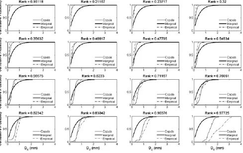
Fig. 8. Sixteen plots of actual coarse-scale pixels with their marginal (field-wide) distribution (thick, black), the empirical distribution of their sub-pixels (thin, dashed) and the modeled distribution of their sub-pixels (thin, solid). The rank of the coarse-scale observation used for conditioning is displayed above each plot.

The EMD is a measure for the minimal cost needed to move all surplus mass to deficit areas, transforming one func-tion into the other. This cost not only accounts for the to-tal mass to be transported (i.e. the vertical difference) but also for the distance between the surplus and the deficit area (i.e. the horizontal difference). Thus, the cost equals the ver-tical distance (the mass) multiplied by the distance it needs to be transported. For the distance measure, weighing functions can be used, however, for this study, all data were binned and the distance was calculated as the absolute difference between the two bin centers. This cost function needs to be minimized in order to find the EMD. This problem is gener-ally known as the transportation problem (Cha and Srihari, 2002; Rubner et al., 2002), and many different specific so-lutions exist such as the Hungarian method (Kuhn, 1955) or the simplex method. These methods find the minimal dis-tance over which the mass needs to be transported, such that the EMD can be found by multiplying the mass transported by the distance it needs to be moved.

5.4.2 Comparison to the field-wide sub-pixel CDF

1454 van den Berg et al.: Copula-based downscaling of spatial rainfall

10

van den Berg et al.: Copula-based downscaling of spatial rainfall

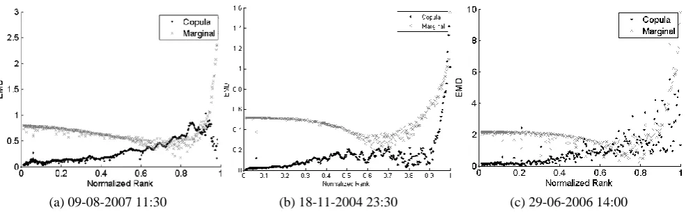
(a) 09-08-2007 11:30 (b) 18-11-2004 23:30 (c) 29-06-2006 14:00

Fig. 9: The EMD between the marginal distribution and the empirical sub-pixel distribution (black crosses) compared to the

EMD of the copula-based, modeled distribution (gray dots).

based performance decreases towards the upper end of the

coarse-scale CDF. This trend is likely due to the imperfect fit

of the marginal distributions and the empirical nature of the

framework (see Sect. 5.2).

The performance has been observed to vary between

dif-ferent rainstorms and even within storms. As an example,

consider Fig. 9a and 9b where two EMD plots are shown

for different storms. Figure 9b shows a fairly typical

per-formance, doing better than the marginal distribution and

showing a fairly typical pattern. However, Fig. 9c shows a

different picture, with a less stable performance. This has

been observed in several cases and seems to be partially due

to instability in the copula as a result of the data.

More-over, the behavior of the performance observed over the

do-main changes between images and storms. Nevertheless,

the copula-based approach generally outperforms the

clas-sical scaling, or has an equal performance. Also, the current

dataset is not amenable to an analysis of the changing

pat-terns prohibiting any further investigation.

5.4.3

Effects of including intermittency

The above section investigated the performance of the

copula-based method without including the intermittence

model. In this section, this model is included in the results

and the EMD computed in a similar fashion to the previous

experiment. The results of this experiment are displayed in

Fig. 10, for the same storm as used in Fig. 8 (results are

simi-lar for all storms). Note that the EMD for the two approaches

is very close for the first part of the curve, clearly due to the

compression of the non-zero part of the distribution. The

patterns in the remainder of the domain remain similar,

al-though a smoothing effect is observed possibly as a result

of the rescaling of the non-zero parts of the CDF. Thus, as

would be expected, the inclusion of intermittency does not

change the performance patterns significantly.

Fig. 10: The EMD after correction for the fraction of dry

pixels.

5.4.4

Temporal robustness of copula

The copula is likely to be specific to a certain storm or

im-age and the performance might be limited by the time lag

between the image on which the copula is fitted and the

im-age to be downscaled. To test this, the copula was fitted to

the first image of a storm and was used to downscale all

se-quential radar images within that same storm. For each of

these images the EMD is calculated on a per pixel basis and

all values are then averaged. In Fig. 12, these values are

displayed for all storms in our dataset, ordered according to

their time-lag. Note that at zero time-lag, i.e. the image from

which the copula is constructed is the same as the image to

be downscaled, the error is not zero. This is partially due to

the empirical nature of the framework, and possibly due to

Hydrol. Earth Syst. Sci., 15, 1–13, 2011

www.hydrol-earth-syst-sci.net/15/1/2011/

values are overestimated (i.e. more high-valued pixels are predicted than should be) by the field-wide distribution. As can be seen from Fig. 8, the copula-based methodology is able to better estimate the varying sub-pixel distributions, providing a closer match to the empirical distribution.

To quantify the performance, the EMD has been com-puted for each coarse-scale pixel for all images analyzed. These values are plotted against the normalized ranks, re-sulting in Fig. 9a, displaying the performance of both the marginal distribution, and that of the copula-based distri-bution. Compared to the marginal distribution, the copula-based distribution has a much more consistent performance over the entire domain and for almost all cases the copula-based method outperforms the fractal-copula-based scaling of the field-wide marginal distribution. Despite this, the copula-based performance decreases towards the upper end of the coarse-scale CDF. This trend is likely due to the imperfect fit of the marginal distributions and the empirical nature of the framework (see Sect. 5.2).

The performance has been observed to vary between dif-ferent rainstorms and even within storms. As an example, consider Fig. 9a and 9b where two EMD plots are shown for different storms. Figure 9b shows a fairly typical per-formance, doing better than the marginal distribution and showing a fairly typical pattern. However, Fig. 9c shows a different picture, with a less stable performance. This has been observed in several cases and seems to be partially due to instability in the copula as a result of the data. More-over, the behavior of the performance observed over the do-main changes between images and storms. Nevertheless, the copula-based approach generally outperforms the clas-sical scaling, or has an equal performance. Also, the current dataset is not amenable to an analysis of the changing pat-terns prohibiting any further investigation.

Fig. 10. The EMD after correction for the fraction of dry pixels.

5.4.3 Effects of including intermittency

The above section investigated the performance of the copula-based method without including the intermittence model. In this section, this model is included in the results and the EMD computed in a similar fashion to the previous experiment. The results of this experiment are displayed in Fig. 10, for the same storm as used in Fig. 8 (results are simi-lar for all storms). Note that the EMD for the two approaches is very close for the first part of the curve, clearly due to the compression of the non-zero part of the distribution. The patterns in the remainder of the domain remain similar, al-though a smoothing effect is observed possibly as a result of the rescaling of the non-zero parts of the CDF. Thus, as would be expected, the inclusion of intermittency does not change the performance patterns significantly.

5.4.4 Temporal robustness of copula

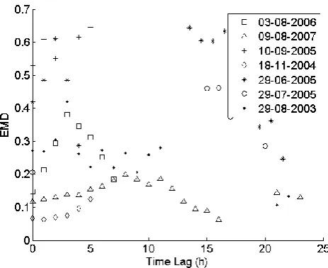
The copula is likely to be specific to a certain storm or im-age and the performance might be limited by the time lag between the image on which the copula is fitted and the im-age to be downscaled. To test this, the copula was fitted to the first image of a storm and was used to downscale all se-quential radar images within that same storm. For each of these images the EMD is calculated on a per pixel basis and all values are then averaged. In Fig. 12, these values are displayed for all storms in our dataset, ordered according to their time-lag. Note that at zero time-lag, i.e. the image from which the copula is constructed is the same as the image to be downscaled, the error is not zero. This is partially due to the empirical nature of the framework, and possibly due to the generalizations inherent to fitting a copula. Despite this, the curves do not appear to have an upward trend, suggesting that an increasing time-lag does not have a negative effect on the performance.

5.4.5 Storm dependence of the copula

Until now, the copula which was used was obtained from the same rain event. To investigate whether the storm used to construct the empirical copula is of importance, a copula was built from 10 different images picked at random from the en-tire dataset. This ensures that the dependence structure gen-erated by different storm types is mixed in order to provide a more general copula. This copula is then applied to several storms and the EMD is calculated for each coarse-scale pixel. The results are displayed in Fig. 11. As can be seen, using the general copula only slightly decreases the overall perfor-mance, but still outperforms the sub-pixel distribution based on scaled marginal distributions. Although more research in this respect is needed, this simple example demonstrates the potential of this scaling technique for downscaling rainfall images in an operational framework, as it may only require to once construct a copula based on a variety of storms.

6 Conclusions

In this paper, a novel technique is introduced which allows for downscaling coarse-scale rainfall images. This method is based on the simultaneous use of fractal-based scaling of the marginal probability distribution functions and a copula which describes the dependence between both scales. The introduction of the dependence allows for a better estimation of the actual shape of sub-pixel probability functions com-pared to the scaled marginal distribution function.

The proposed method can strengthen current downscaling methods which assume unrealistic sub-pixel distributions. This will require at least a moderate degree of temporal sta-bility of the copula, which has been tentatively shown in this study. Future research will focus on this temporal stabil-ity and it will be investigated whether different copulas are

Fig. 11. The EMD between the empirical sub-pixel distribution and the specifically fitted copula (gray dots), the more general copula (black dots), or the field-wide marginal distribution (black crosses).

Fig. 12. The EMD determined for every image of each storm (dates listed in the legend) with the copula used for all images in a single storm based on the first image of that storm.

needed for different storm types and whether the same scal-ing can be applied for different storm types. As such, fu-ture work should not only include a larger dataset, but also involve storm classification to investigate differences in de-pendence structure between storms.

1456 van den Berg et al.: Copula-based downscaling of spatial rainfall be known. Therefore, a function is needed that relates the

parameters of the parametrical copulas to the scales between which these are valid. Future research should also focus on whether a parametrical copula can be fitted such that prob-lems at the extremes of the copula, where little data is avail-able, are solved.

It was shown that the copula-based framework is suffi-ciently robust to be applied to different storms and time steps, demonstrating its large potential for statistical downscaling and hydrological modeling. Yet, more research is needed to further elaborate the proposed methodology.

Acknowledgements. The first author was supported by the Special

Research Fund of Ghent University, and the second author was funded by Research Foundation Flanders (FWO). The authors kindly thank the Royal Meteorological Institute of Belgium for providing the data.

Edited by: F. Pappenberger

References

Allcroft, D. and Glasbey, C.: A latent Gaussian Markov random-field model for spatiotemporal rainfall disaggregation, J. R. Stat. Soc. C-App., 52, 487–498, doi:10.1111/1467-9876.00419, 2003. Burton, A., Kilsby, C. G., Fowler, H. J., Cowpertwait, P. S. P., and Connell, P. E. O.: RainSim : A spatial temporal stochastic rain-fall modelling system, Environ. Modell. Softw., 23, 1356–1369, doi:10.1016/j.envsoft.2008.04.003, 2008.

Cha, S. H. and Srihari, S. N.: On measuring the dis-tance between histograms, Pattern Recogn., 35, 1355–1370, doi:10.1016/S0031-3203(01)00118-2, 2002.

Collison, A., Steven, W., Griffiths, J., and Dehn, M.: Mod-elling the impact of predicted climate change on landslide fre-quency and magnitude in SE England, Eng. Geol., 55, 205–218, doi:10.1016/S0013-7952(99)00121-0, 2000.

Cowpertwait, P. S. P., Kilsby, C. G., and O’Connell, P. E.: A space-time Neyman-Scott model of rainfall: Empiri-cal analysis of extremes, Water Resour. Res., 38, 1131, doi:10.1029/2001WR000709, 2002.

De Jongh, I. L. M., Verhoest, N. E. C., and De Troch, F. P.: Analy-sis of a 105-year time series of preceipitation observed at Uccle, Belgium, Int. J. Climatol., 26, 2023–2039, doi:10.1002/joc.1352, 2006.

De Michele, C. and Salvadori, G.: A generalized pareto intensity-duration model of storm rainfall exploiting 2-copulas, J. Geo-phys. Res., 108, 4067, doi:10.1029/2002JD002534, 2003. Deidda, R.: Rainfall downscaling in a space-time

multi-fractal framework, Water Resour. Res., 36, 1779 –1794, doi:10.1029/2000WR900038, 2000.

Deidda, R., Benzi, R., and Siccardi, F.: Multifractal modeling of anomalous scaling laws in rainfall, Water Resour. Res., 35, 1853–1867, doi:10.1029/1999WR900036, 1999.

Ferraris, L., Gabellani, S., Rebora, N., and Provenzale, A.: A comparison of stochastic models for spatial rainfall downscaling, Water Resour. Res., 39(12), 1368, doi:10.1029/2003WR002504, 2003a.

Ferraris, L., Gabellani, S., Parodi, U., Rebora, N., von Harden-berg, J., and Provenzale, A.: Revisiting multifractality in rain-fall fields, J. Hydrometeorol., 4, 544–551, doi:10.1175/1525-7541(2003)004<0544:RMIRF>2.0.CO;2, 2003b.

Gao, H., Wood, E. F., Drusch, M., and McCabe, M. F.: Copula-derived observation operators for assimilating TMI and AMSR-E retrieved soil moisture into land surface models, J. Hydrometeo-rol., 8, 413–429, doi:10.1175/JHM570.1, 2007.

Genest, C. and Favre, A.: Everything you always wanted to know about copula modeling but were afraid to ask, J. Hydrol. Eng., 12, 347–368, doi:10.1061/(ASCE)1084-0699(2007)12:4(347), 2007.

Gibbs, A. L. and Su, F. E.: On Choosing and Bounding Prob-ability Metrics, International Statistical Review, 70, 419–435, doi:10.1111/j.1751-5823.2002.tb00178.x, 2002.

Grimaldi, S. and Serinaldi, F.: Asymmetric copula in multivariate flood frequency analysis, Adv. Water Resour., 29, 1155–1167, doi:10.1016/j.advwatres.2005.09.005, 2006.

Gupta, V. K. and Waymire, E.: Multiscaling properties of spatial rainfall and river flow distribution, J. Geophys. Res., 95, 1999– 2009, doi:10.1029/JD095iD03p01999, 1990.

Heylen, R. and Maenhout, A.: Inleiding tot de radarmeteorologie, Koninklijk Meteorologisch instituut van Belgie, Brussels, 69 pp., 1994 (in Dutch).

Kao, S. and Govindaraju, R. S.: Trivariate statistical analysis of extreme rainfall events via the Plackett family of copulas, Water Resour. Res., 44, W02415, doi:10.1029/2007WR006261, 2008. Kuhn, H. W.: The Hungarian method for the assignment problem,

Nav. Res. Logist. Q., 2, 83–97, doi:10.1002/nav.3800020109, 1955.

Le Cam, L.: A stochastic description of precipitation, in: Proceed-ings of the Fourth Berkeley Symposium on Mathematical Statis-tics and Probability, vol. 3, 165–186, 1961.

Lovejoy, S. and Mandelbrot, B.: Fractal properties of rain and a fractal model, Tellus, 37, 209–232, doi:10.1111/j.1600-0870.1985.tb00423.x, 1985.

Mackay, N. G., Chandler, R. E., Onof, C., and Wheater, H. S.: Dis-aggregation of spatial rainfall fields for hydrological modelling, Hydrol. Earth Syst. Sci., 5, 165–173, doi:10.5194/hess-5-165-2001, 2001.

Marshall, J. and Palmer, W.: The distribution of raindrops with size, J. Atmos. Sci., 5, 165–166, doi:10.1175/1520-0469(1948)005<0165:TDORWS>2.0.CO;2, 1948.

Menabde, M., Seed, A., and Pegram, G.: A simple scaling model for extreme rainfall, Water Resour. Res., 35, 335–339, doi:10.1029/1998WR900012, 1999.

Nelsen, R. B.: An introduction to copulas, Springer Verlag, 2006. Onof, C., Mackay, N. G., Oh, L., and Wheater, H. S.: An improved

rainfall disaggregation technique for GCMs, J. Geophys. Res., 103, 19577–19586, doi:10.1029/98JD01147, 1998.

Onof, C., Chandler, R. E., Kakou, A., Northrop, P., Wheater, H. S., and Isham, V.: Rainfall modelling using Poisson-cluster pro-cesses: a review of developments, Stoch. Env. Res. Risk A., 14, 384–411, doi:10.1007/s004770000043, 2000.

Pegram, G. G. S. and Clothier, A. N.: Downscaling rainfields in space and time, using the String of Beads model in time series mode, Hydrol. Earth Syst. Sci., 5, 175–186, doi:10.5194/hess-5-175-2001, 2001.

Rebora, N., Ferraris, L., von Hardenberg, J., and Provenzale, A.:

RainFARM: rainfall downscaling by a filtered autoregressive model, J. Hydrometeorol., 7, 724-738, doi:10.1175/JHM517.1, 2006.

Rubner, Y., Tomasi, C., and Guibas, L.: A metric for distributions with applications to image databases, in: Computer Vision, Sixth International Conference on, 59–66, IEEE, 2002.

Salvadori, G. and De Michele, C.: Statistical characterization of temporal structure of storms, Adv. Water Resour., 29, 827–842, doi:10.1016/j.advwatres.2005.07.013, 2006.

Salvadori, G. and De Michele, C.: On the use of copulas in hy-drology: theory and practice, J. Hydrol. Eng., 12, 369–380, doi:10.1061/(ASCE)1084-0699(2007)12:4(369), 2007. Schertzer, D. and Lovejoy, S.: Physical modeling and analysis of

rain and clouds by anisotropic scaling multiplicative processes, J. Geophys. Res., 92, 9693–9714, doi:10.1029/JD092iD08p09693, 1987.

Sch¨olzel, C. and Friederichs, P.: Multivariate non-normally dis-tributed random variables in climate research – introduction to the copula approach, Nonlin. Processes Geophys., 15, 761–772, doi:10.5194/npg-15-761-2008, 2008.

Serinaldi, F.: Copula-based mixed models for bivariate rainfall data: an empirical study in regression perspective, Stoch. Env. Res. Risk A., 23, 677–693, doi:10.1007/s00477-008-0249-z, 2009. Vandenberghe, S., Verhoest, N. E. C., Buyse, E., and De Baets,

B.: A stochastic design rainfall generator based on copulas and mass curves, Hydrol. Earth Syst. Sci., 14, 2429–2442, doi:10.5194/hess-14-2429-2010, 2010.a.

Vandenberghe, S., Verhoest, N. E. C., and De Baets, B.: Fitting bi-variate copulas to the dependence structure between storm char-acteristics: A detailed analysis based on 105 year 10 min rainfall, Water Resour. Res., 46, W01512, doi:10.1029/2009WR007857, 2010b.

Varis, O., Kajander, T., and Lemmel¨a, R.: Climate and water: from climate models to water resources man-agement and vice versa, Climatic Change, 66, 321–344, doi:10.1023/B:CLIM.0000044622.42657.d4, 2004.

Veneziano, D., Langousis, A., and Furcolo, P.: Multifractality and rainfall extremes: A review, Water Resour. Res., 42, W06D15, doi:10.1029/2005WR004716, 2006.

Vrac, M. and Naveau, P.: Stochastic downscaling of precipita-tion: From dry events to heavy rainfalls, Water Resour. Res., 43, W07402, doi:10.1029/2006WR005308, 2007.

Wilks, D. S.: Multisite downscaling of daily precipitation with a stochastic weather generator, Clim. Res., 11, 125–136, doi:10.3354/cr011125, 1999.

Willems, P.: A spatial rainfall generator for small spatial scales, J. Hydrol., 252, 126–144, doi:10.1016/S0022-1694(01)00446-2, 2001.