Error Correction for Symbolic and Hybrid Symbolic-Numeric Sparse Interpolation Algorithms.

(1)

Abstract

COMER, MATTHEW T. Error Correction for Symbolic and Hybrid Symbolic-Numeric Sparse Interpolation Algorithms. (Under the direction of Erich L. Kaltofen.)

We introduce error correction to two problems of sparse polynomial interpolation. In the first problem, we recover at-sparse polynomial f(x) (in the power basis) from valuesf(ωi−1_),

i= 1,2, . . . ,2t(2E+ 1), whereω is a field element of our choice, and at most E values contain random/misleading errors. Our algorithm is adapted from the linear recurrence-based algorithm of [Prony III (1795),J. de l’ ´Ecole Polytechnique, 1:24-76]. In the exact setting, error correction is implemented directly in the computation of the minimal generator of the linearly recurrent sequence {f(ωi−1_{)}. In the numeric setting, where every evaluation is perturbed by a small}

relative “noise” error and at most E evaluations are perturbed by large “outlier” errors, we appeal to the results of [Kaltofen and Lee 2003, J. Symbolic Comput., 36(3-4):365-400] and [Kaltofen, Lee, and Yang 2011,Proc. 2011 Internat. Workshop on Symbolic-Numeric Comput., pages 130-136] for computation of the approximate minimal generator.

In the second problem, we compute a shift s that will yield the sparsest representation of a polynomial f(x) in the shifted power basis (x−s)k_{. To this end, two algorithms are} pre-sented. The first algorithm computes the representation from polynomialsf(ωi₊_z)_∈_F_{[z]. The} polynomials are interpolated densely, using Blahut’s decoding method for Reed-Solomon error-correction, then the shiftsand sparsitytare computed from the error-free “values”f(ωi−1_+z),

where now i = 1,2, . . . ,2t+ 1. The second step employs the results of [Giesbrecht, Kaltofen, and Lee 2003, J. Symbolic Comput., 36(3-4):401-424]. The second algorithm takes advantage of the representation f(x) = Pt_i₌₁ci(x−s)ei being the Taylor expansion of f(x) at x = s. Erroneous evaluations are detected by first interpolating f(x) densely, then comparing all eval-uations to their corresponding values of the interpolant. Both algorithms have adaptations for the numeric setting; the first algorithm relies on results of [Hutton, Kaltofen, and Zhi 2010, Proc. 2010 Internat. Symp. Symbolic Algebraic Comput., pages 227-234] to determine the shift and sparsity.

(2)

Error Correction for Symbolic and Hybrid Symbolic-Numeric Sparse Interpolation Algorithms

by

Matthew T. Comer

A dissertation submitted to the Graduate Faculty of North Carolina State University

in partial fulfillment of the requirements for the Degree of

Doctor of Philosophy

Applied Mathematics

Raleigh, North Carolina 2013

APPROVED BY:

Erich L. Kaltofen

North Carolina State University Chair of Advisory Committee

Irina A. Kogan

North Carolina State University

Wen-shin Lee University of Antwerp

Michael F. Singer

North Carolina State University

Ralph C. Smith

(3)

Dedication

(4)

Biography

(5)

Acknowledgements

First, I thank my advisor for his mentoring and support during productive times, his patience and understanding during the challenging times, and for sharing his original ideas, for which I will always be grateful. In addition, I thank him for his advice and guidance well after the defense, both in time and scope. Thank you, Erich.

I thank my Ph.D. committee for their time and consideration, and for their comments and suggestions during the preliminary and final oral exams. Thank you, Irina Kogan, Wen-shin Lee, Jon Rust, Michael Singer, Charles Smith, and Ralph Smith.

I thank our collaborators and friends for the opportunities to share the research process with them and to learn from them. Thank you, Brice Boyer, Feng Guo, and Cl´ement Pernet.

I thank everyone who supported me in each facet of my research experiences, which have taken me not only around the USA, but also China and France. From travel to mentoring to conversation to advice, thank you, all.

I thank the professors of my courses at North Carolina State University, who taught me not only the content and skills appropriate for each course, but also general skills and strategies that have helped me throughout all of the mathematics that I have encountered in my career thus far. Thank you, all.

I thank my fellow students at North Carolina State University for forming a support group beyond measure. I will always fondly reminisce our experiences together, both curricular and extracurricular. Thank you, friends.

I thank professors Keith Conrad and Joe McKenna at the University of Connecticut for their guidance and advice about upper-level math courses, undergraduate research, and graduate school. Thank you, both.

I thank all of my friends and professors at the University of Connecticut for inspiring my passion for mathematics, and further inspiring me to apply to graduate school. Thank you, all.

I thank my family for their love and support throughout all of my education, especially the graduate school years. Thank you, all.

(6)

List of Tables

(9)

List of Figures

(10)

Chapter One

Introduction

Error-correcting decoding is ubiquitous in modern computing. With polynomial interpolation being used as a key step for error-correcting decoding, it is a natural extension to account for errors in the process of polynomial interpolation itself. Without errors, the process of recovering a polynomial from a sampling of its points has been studied in various contexts. For example, to interpolate a polynomialf(x) of degree less than d, one could obtaindevaluations of f(x) (at distinctx-values) and then solve a Vandermonde system to produce a representation off(x). It is important to note that givenanyset ofdpoints (again, for distinctx-values), a Vandermonde system will yield a polynomial of degree less thandthat passes through each point: one cannot simply inspect the proposed interpolant to determine if some evaluations were faulty.

As with many schemes of error-correcting (de)coding, the introduction of redundancy en-ables the problem of error-correcting interpolation to become more tractable. Specifically, if we wish to interpolate a polynomial of degree less thand, but we have a boundE on the maximum number of erroneous evaluations in a given set, then obtaining d+ 2E evaluations guarantees that there can be only oneE-error interpolant (i.e., a polynomial that passes through all but k points, wherek≤E). For suppose there were twoE-error interpolants, f(x) and g(x), each of degree less than d. Then it must be that f and g agree for at least dpoints, which implies f = g (because the polynomial f −g, also of degree less than d, has at least d roots). As a counter-example ford=E= 1, consider thed+ 2E−1 = 2 points (x1, y1) and (x2, y2), where

x1 6=x2 andy1 6=y2. Thenf(x) =y1 and g(x) =y2 are each a 1-error interpolant for the set of

two points. One can generalize this example for arbitrary dand E (starting withd−1 points common to f and g, then including E points unique to each of f and g) to show that d+ 2E points are necessary and sufficient to guarantee uniqueness of the interpolant.

(11)

optimization problem of minimizing the number of evaluations needed to recover the unique interpolant. Knowing only that a polynomial is of degree less than d, one generally requires d points for interpolation. However, if we know that the polynomial has few terms compared to its degree – that is, the polynomial is sparse – then the minimum number of evaluations may be decreased, due to a phenomenon discovered by Prony during the French Revolution. In [Prony III (1795)], it is shown that one can interpolate a sum of t exponential functions, say, f(x) = Pt_i₌₁cibx

i, from only 2t evaluations. Here, Prony used not an arbitrary set of evaluations, but rather a sequence of evaluations at consecutive multiples of a single x-value: 0, α,2α, . . . ,(2t−1)α.

Prony showed that this sequence of evaluations satisfies a particular recurrence relation: if we denote the evaluations by ai=f(iα), then

γ0a0+i+γ1a1+i+. . .+γt−1at−1+i+at+i = 0, i= 0,1, . . . , t−1,

for some constantsγi. (More accurately, the sequence satisfies ahomogeneous linear recurrence relation with constant coefficients, which will continue to be called simply a recurrence relation, and such a sequence will be called simply a linearly recurrent sequence.) By examining the ratios a1/a0, a2/a0, . . . , a2t−1/a0, Prony derived explicit formulas for the γi and showed that

the polynomial Λ(λ) = Pt_i−1₌₀γiλi

+λt _{factors as Λ(λ) =}Qt

i=1(λ−bαi). Thus, from only the sequence of evaluations, one can determine (through formulas and polynomial factorization) all of the bases bi. Equivalently, if we re-write f(x) = Pt_i₌₁cibeix_{, where} _ei _{= log}

b(bi), then we have Λ(λ) =Qt_i₌₁(λ−be1α_{), so that we wish to recover the exponents}_e

i.

A special case ist= 1: the recurrence relation is given byγ0ai =ai+1, so that the sequence

is geometric. Indeed,

f (n+ 1)α

f(nα) =

c1b(n+1)αe1

c1bnαe1

= (b

αe1₎n+1 (bαe1₎n =b

αe1_,

from which one can recover e1 (knowing band α). Then the only unknown quantity inf(x) =

c1be1xisc1, which can be recovered immediately froma0 =c1. For generalt, one computes the

ex-ponentse1, e2, . . . , etfrom the 2tevaluations, then one can compute the coefficientsc1, c2, . . . , ct

from any subset of tevaluations (e.g., by solving a t×t Vandermonde system). To relate this result to polynomials, we note that if we substitute α= log_b(ω), then this becomes

f log_b(ωn+1₎

f logb(ωn)

=blogb(ω)e1 ₌_ωe1 ₌ g(ω

n+1₎

g(ωn₎ , forg(x) =c1x e1_.

(12)

sparse functions in an exponential or polynomial basis, the focus is the computation of the re-currence relation amonga0, a1, . . . , a2t−1. Furthermore, if some of the evaluations are erroneous,

then we must have some method of accounting for errors in the recovery of the recurrence re-lation. By introducing redundancy as in the general/dense polynomial example above, we are able to detect and correct errors, but we appeal to a more modern algorithm for computing a recurrence relation.

Seventeen decades after Prony’s discovery, Berlekamp introduced a decoding method for multiple-error-correcting binary Bose-Chaudhuri-Hocquenghem (BCH) codes; Algorithm 7.4 of [Berlekamp 1968] is presented for determining the shortest feedback-shift-register (i.e., minimal recurrence relation) of a sequence of digits representing the (possibly erroneous) transmission of a codeword. (Such a minimal recurrence relation exists due to the module structure of the space of all sequences being acted-on by the univariate polynomial ring; see, e.g., Section 12 of [von zur Gathen and Gerhard 1999].) In Berlekamp’s formulation, the recurrence relation gives the coefficients of the “error locator polynomial” (also called the generator of the sequence), whose roots are the reciprocals of Galois field elements that represent the locations where errors occurred.

One immediate advantage over Prony’s method is that Berlekamp’s algorithm iterates through the sequence, processing one entry at a time: for each n= 1,2, . . ., the minimal gen-erator is found for the first n entries of the sequence, using the computations that produced the generator for the first n−1 entries (where the generator for n= 0 is the polynomial 1 by convention). Berlekamp proved that the degree of the minimal generator (equivalently, length of the minimal recurrence relation) could be computed at the beginning of each iteration by testing if the generator for nentries continues to generate the (n+ 1)-st entry.

Whereas Berlekamp’s algorithm was intended for sequences that arise in BCH decoding, Massey generalized Berlekamp’s algorithm to the realm of arbitrary linearly generated se-quences, granting the name “Berlekamp Iterative Algorithm” (see Section III of [Massey 1969]), which later adopted the name Berlekamp/Massey Algorithm. Through direct manipulation of recurrence relations, Massey showed that the degree of the minimal generator follows a concise rule: if we denote by Ln(a) the degree of the minimal generator for the first n entries of the sequence a, then Ln+1(a) = max{Ln(a), n+ 1−Ln(a)}. This property allows the iterative

step of the Berlekamp/Massey Algorithm to depend on a simple switch: whether or not there is a length change (i.e., Ln+1 > Ln). It is the nature of this length change test that allows us to introduce error correction to the minimal generator computation: eventually in a linearly generated sequence, a single error will cause a large increase in the length of the generator.

In Chapter 2, we formally define the problem of error correction for linearly generated sequences: suppose that a sequencea0, a1, . . .of elements from a field,F, has a minimal generator

(13)

recover Λ (theintendedgenerator) and correct the errors in the sequence. (Counter-)examples1

and2show that one must haven≥2t(2E+1) for the problem to have a unique solution, at least when char(F₎ _{6= 2. Given this lower bound on} _{n, the determination of the intended generator} amounts to a “majority vote” of generator candidates obtained by executing the Berlekamp/ Massey algorithm on each contiguous subsequence of 2t entries; this follows from Lemma3.

After recovering the intended generator, detection and correction of errors is not as simple as applying the generator to the entire sequence {bi}, changing entries as necessary to fit the recurrence. Rather, it may be that an erroneous “block” of 2t entries yields the intended generator. For example, consider the two sequences

¯

0, 0, 1, ¯0, 0, 2 ¯

0, 1, 1, ¯0, 2, 2 , ¯ 0 =

t−2 times

z }| {

0, . . . ,0,

both of which yield−2+λt_{as minimal generator. Suppose the entire intended sequence}_{ai}_were a continuation of the first sequence (using−2+λt_{to generate further entries), but the erroneous} sequence {bi} were formed by substituting the first block as above. Testing the generator with the first block as initial input, the recurrence would fail at locations that agree with the intended sequence. We call such a block as above a “deceptive block”; Theorem4proves that a deceptive block will cause more than E such failure locations, so that one will know to use a different block as initial input to the generator test. It is also proven that the method works when only a boundT ≥tis known.

Thus having an error-correction strategy for linearly generated sequences, Prony’s method becomes part of an error-correcting algorithm for sparse interpolation. We describe the full algo-rithm as an adaptation of Ben-Or’s & Tiwari’s algoalgo-rithm for error-free sparse interpolation (see [Ben-Or and Tiwari 1988]), which applies Prony’s method to the multivariate case, substituting a distinct prime for each variable.

We also explore a numeric/approximate adaptation of the univariate case, where we choose ωto be an appropriate complex root of unity (for numerical stability); Section2.6describes the algorithm and presents some experiments where every evaluation is perturbed by a (relatively) small “noise” error, while only a few evaluations are perturbed by a (relatively) large “outlier” error. It should be noted that when the evaluations are only approximate, the Berlekamp/ Massey algorithm cannot be directly implemented, as it includes an explicit test for zero (when determining whether a recurrence relation holds); thus, we appeal to the results of [Kaltofen and Lee 2003] and [Kaltofen, Lee, and Yang 2011] to compute the approximate minimal generator. Also, it may be that the majority vote is inconclusive, so we appeal to oversampling: several sequences of evaluations are obtained, substituting different values for ω.

(14)

unity causes the sparse interpolation with errors problem to be dual to that of decoding Reed-Solomon codes, as shown in Section 2.3. With a result of [Blahut 1983], we present the sparse interpolation with errors problem from the perspective of error-correcting coding.

Whereas Chapter2addresses the problem of sparse polynomial interpolation with errors in the power basis (1, x, x2, . . .), Chapter 3 addresses a similar problem, but in the shiftedpower basis: 1,(x−s),(x−s)2_{, . . .}_{for some constant value} _{s, which is a priori unknown. This results}

in an optimization problem: find the value of s that yields the fewest terms in the shifted representationf(x) =Pt_i₌₁ci(x−s)ei_.

For a first interpolation algorithm, we appeal to the results of [Kaltofen and Lee 2003]. Consider that g(x) = f(x+s) is sparse in the (un-shifted) power basis, so the sequence of evaluationsa0=g(1), a1 =g(ω), a2=g(ω2), . . .is linearly generated by Λ(λ) =Qti=1(λ−ωei).

Equivalently, the Hankel matrix Hm = [ai+j−2]mi,j=1 is singular for m = t+ 1, with a column

relation given by the coefficients of Λ. Furthermore, Theorem 4 of [Kaltofen and Lee 2003] states that, with high probability, Hm is non-singular for 1 ≤ m ≤ t when ω is randomly sampled from a sufficiently large subset ofF_.

In [Giesbrecht, Kaltofen, and Lee 2003], by defining two sequences ai = f(ωi

1 +z) and

bi = f(ωi

2 +z) with z an indeterminate for s and ω1, ω2 each randomly sampled, it is shown

that (again, with high probability) if one computes the GCD of the determinants of them×m Hankel matrices formed by the two sequences, then z+s will be the first non-trivial GCD, exactly when m = t+ 1. To introduce error correction in the function evaluations, we pre-condition the evaluations by performing dense interpolation with errors (based on Blahut’s method for decoding Reed-Solomon codes) onf(ωi+z), as a dense polynomial inz.

If we view the representationf(x) =Pt_i₌₁ci(x−s)ei _{as the Taylor expansion of}_f _at_x₌_s,

then we see thats must be a root of all derivatives of f whose order is not some ei. Thus, we search for the root where the most derivatives vanish, which immediately gives all valuesei as well. If f has no more than half the possible number of terms, then Theorem 1 of [Lakshman Y. N. and Saunders 1996] guarantees that the value of sis unique and rational. We show that one need compute only the 2t highest-order derivatives (the highest being the (deg(f)−1)-st derivative in this context) to finds, with the possibility of early termination. To compute these derivatives without having knowledge ofs, one would need methods of dense interpolation with errors to compute the 2t highest-order terms of f. Due to the necessary division in Taylor coefficients, we restrict this algorithm to fields of characteristic zero.

(15)

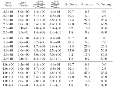
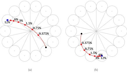
polynomial interpolation, where the exponents of the sparse polynomial correspond to the error locations in the sequence of dense polynomial evaluations. In particular for the numeric setting, we explore the relative difference between the magnitudes of noise and outlier in the 1-outlier case, giving a sufficient condition that will guarantee recovery of the error location. We show some experiments of what can happen when the magnitude of an outlier approaches that of general noise.

Chapter 4 addresses the problem of enumerating square singular Hankel matrices with entries from a finite field F_{q, specifically when some of the anti-diagonals may be fixed to} particular values. Though not directly related to sparse interpolation, the solution is intimately connected to the Berlekamp/Massey algorithm, as a Hankel matrix H = [ai+j−2]ni,j=1 can be

represented by the sequence a0, a1, . . . , a2n−2. By executing the Berlekamp/Massey algorithm

on the sequence, one can determine which leading principal submatrices ofH are non-singular, due to Lemma 2 of [Kaltofen and Yuhasz 2013a]: there will be a length change, Lm > Lm−1,

exactly when theLm×Lm leading principal submatrix is non-singular.

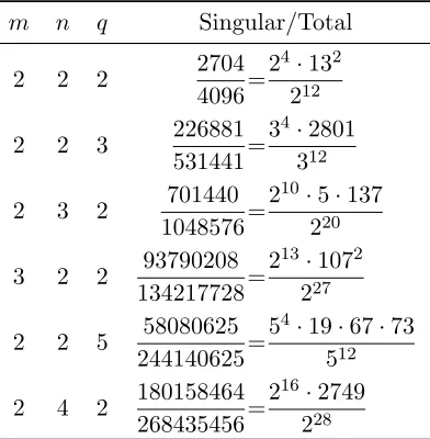
We use this property to determine, for any singular Hankel matrix, a unique anti-diagonal that, if changed to any of the otherq−1 values in F_{q, will cause the matrix to be non-singular.} This induces a map from the set of singular Hankel matrices to the power set of non-singular Hankel matrices (see Section4.3). By showing that the images of the map will partition the set of non-singular matrices, we can prove the already-established property that a fraction of 1/q of all Hankel matrices are singular. In addition, because the singularity-controlling anti-diagonal is found on or below the main diagonal, we can determine singularity when any of the anti-diagonals on or above the main anti-diagonal are fixed (while the other anti-anti-diagonals range overF_{q). Theorem}₅_{shows the three cases for counting square singular Hankel matrices, which} depend on the choice of fixed anti-diagonals and the values of those anti-diagonals. The result is analogous when some anti-diagonals are fixed on or below the main anti-diagonal, but not when anti-diagonals above and below the main anti-diagonal are fixed.

(16)

Chapter Two

Sparse Polynomial Interpolation

with Noise and Outliers (

SPINO

)

This chapter is [Comer, Kaltofen, and Pernet 2012], except for the modifications listed in Note2.

2.1 Introduction

The problem of reconstructing a sparse polynomial from its values stands at the nexus of symbolic and numeric computing. The astounding success of the numerical versions of the exact symbolic sparse interpolation algorithms [Grigoriev and Karpinski 1987; Ben-Or and Tiwari 1988;Kaltofen, Lakshman Y. N., and Wiley 1990;Kaltofen and Lee 2003], namely the “GLL”-algorithm [Giesbrecht, Labahn, and Lee 2009], in medical signal processing by Annie Cuyt, Wen-shin Lee, and others (see, e.g., http://smartcare.be) leads to a statistical problem variant: allow for outlier measurement errors in addition to noise.

2.1.1 Exact Sparse Interpolation With Errors

(17)

is based on Ben-Or’s and Tiwari’s (1988) algorithm, which computes the sparse support (the set of non-zero terms) via a linear recurrence. We compute the linear generators for multiple segments of the sequence to expose the faults in some of the segments.

We also study on its own the Berlekamp/Massey algorithm on input sequences with faulty elements, and show that uniqueness of a linear generator of degreetcannot be guaranteed from a sequence segment of <2t(2e+ 1) consecutive elements with eerrors. For sequence segments of ≥ 2T(2E+ 1) consecutive elements with e ≤ E errors, we not only can easily recover the unique linear generator of degreet≤T where the boundsT, E are input, but we can also locate and correct the errors. For sequences arising in sparse interpolation, fewer elements may suffice for a unique interpolant, as we do not have the corresponding counterexamples.

The exact dense interpolation problem with errors is studied in [Khonji, Pernet, Roch, Roche, and Stalinsky 2010]. The exact sparse problem is also investigated in [Saraf and Yekhanin 2011], where it is assumed, as we do not, that the support of the sparse polynomial is known. However, Saraf’s CCC ’11 talk has motivated our investigations.

2.1.2 The Nature of Noise

In numerical data, noise is a result of imprecise measurement or of floating point arithmetic. It is assumed that there is some accuracy in the data. In digital data, noise spoils several bits and accuracy is measured as having a small Hamming distance. When approximating a transcendental function by a Taylor series or Pad´e fraction, noise is the model error of the inexact representation. Hybrid symbolic-numeric algorithms have traditionally assumed that the input scalars have with some relative error been deformed. For instance, if one allows substantial oversampling, a sparse polynomial can be recovered from numerical noisy values, where each value has a relative error of 0.5 [Giesbrecht and Roche 2011], perhaps even 0.99, with still more oversampling. Here we consider errors in the Hamming distance sense, i.e., several incorrect values without assumption on any accuracy. But we can combine our model with that of numerical noise in all other values, hence we borrow the statistical termoutlierfor the nature of these errors.

(18)

2.1.3 Numeric Sparse Interpolation

Linear recurrence-based sparse interpolation goes back to the French revolution [Prony III (1795)]. In fact, Prony’s algorithm is Ben-Or’s/Tiwari’s if one replaces the polynomial variables

by exponential functions x = ey_{. For imaginary replacements} _x ₌ _ei_y

one obtains periodic sparse sinusoid (finite Fourier) signals (cf. [Cadzow 1988]). Prony’s algorithm disappeared from numerical analysis books for reason of conditioning [Wen-shin Lee, private communication]. The probabilistic analysis of the randomized early termination algorithm [Kaltofen and Lee 2003] together with analysis of the distribution of the corresponding condition numbers [Giesbrecht, Labahn, and Lee 2009; Kaltofen, Lee, and Yang 2011] now justifies its use, even numerically. Ill-conditioning arises precisely at the point of termination, and condition number estimation or stochastic input sensitivity analysis can be used to identify this point. Already Prony’s paper shows that the sparse terms can have negative, and possibly rational, exponents.

2.1.4 Numeric Outliers

Important variants of our algorithms can deal with numerical noise, from floating point or empirical input values, and outliers. We demonstrate that the Prony-GLL style algorithms [Giesbrecht, Labahn, and Lee 2009;Kaltofen, Lee, and Yang 2011] are applicable to our major-ity voting approach by describing our early-terminated numeric version of the Ben-Or/Tiwari Algorithm; some particular examples are given in Section 2.6.

2.1.5 The Ben-Or/Tiwari Algorithm

We briefly review Ben-Or’s/Tiwari’s algorithm in the setting of univariate sparse polynomial interpolation. Let f be a univariate polynomial, mj its distinct terms, t the number of terms, and cj the corresponding non-zero coefficients:

f(x) = t

X

j=1

cjxej = t

X

j=1

cjmj 6= 0, ej ∈Z.

Theorem 1. [Ben-Or and Tiwari 1988] Let bj = ωej, where ω is a value from the coefficient domain to be specified later, let ai = f(ωi_{) =} Pt

j=1cjbij, and let Λ(λ) =

Qt

j=1(λ−bj) =

λt+γt−1λt−1+· · ·+γ0. The sequence(a0, a1, . . .)is linearly generated by the minimal polynomial

Λ(z).

The Ben-Or/Tiwari algorithm then proceeds in the four following steps:

1. Find the minimal-degree generating polynomial Λ for (a0, a1, . . .), using the Berlekamp/

(19)

2. Compute the rootsbj of Λ, using univariate polynomial factorization. 3. Recover the exponents ej of f, by repeatedly dividingbj byω.

4. Recover the coefficients cj off, by solving the transposed t×t Vandermonde system

      

1 1 . . . 1

b1 b2 . . . bt ..

. ... . .. ... bt₁−1 bt₂−1 . . . bt_t−1

              c1 c2 .. . ct        =        a0 a1 .. . at−1

       .

By Blahut’s theorem [Blahut 1979;Massey and Schaub 1988], the sequence (ai)i≥0has linear

complexityt, hence only 2t coefficients suffice for the Berlekamp/Massey algorithm to recover the minimal polynomial Λ. In the presence of errors in some of the evaluations, this fails. Our work shows how to overcome that obstruction.

2.2 Length Bounds for Computing Linear Generators From

Se-quences with Error

2.2.1 Necessary Length of the Input Sequence

Example 1. Suppose the base field is F_{, where char(}F₎ _{6= 2. Given} _{e, t}_≥ _{1, let ¯}_{0 denote the} zero vector of lengtht−1. Consider the following sequence of length 4t:

(¯0,1,¯0,_|{z}1

−1

,¯0,1,¯0,

1

z}|{

−1 ) ⇒ −1 + λt ⇒1 +λt

.

Here, the underbrace and overbrace represent distinct “corrections” that would yield two different minimal linear generators (1 +λt _and _{−1 +}_λt_{, respectively). If we concatenate this} sequence with itselfe−1 times, then append the sequence (¯0,1,¯0), the result is a sequence of length 4et+ 2t−1 = 2t(2e+ 1)−1, where two sets of “corrections” would each yield a different minimal linear generator. Thus, at least 2t(2e+ 1) sequence entries are necessary to guarantee a unique solution.

Example 2. Suppose again that the base field isF_{, where char(}F₎_{6= 2. Let} _α _{be an}_{e-th root} of unity, for eeven, and consider the following sequence of 2(2e+ 1)−1 entries:

(20)

If the odd powers of −α are changed to odd powers of α, then −α+λis the minimal linear generator. However, if the odd powers ofαare changed to odd powers of −α, thenα+λis the minimal linear generator. Note that there are e changes made to the sequence in either case. Thus, at least 2(2e+ 1) entries are required to guarantee a unique solution whent= 1.

For the case t > 1, we place the zero-vector of length t−1 in between each entry above, and on each end of the sequence. Again, we see that at least 2t(2e+ 1) entries are required to guarantee a unique solution.

As an explicit example, let e= 4, t= 1, and consider the following sequence:

(1, i

|{z}

−i

,−1, −i

|{z}

i

,1,

i

z}|{

−i _,_−1, −i

z}|{

i _,_1, i

|{z}

−i

,−1, −i

|{z}

i

,1,

i

z}|{

−i _,_−1, −i

z}|{

i _,_1).

When eis odd, we can take the example for e+ 1, remove the last 4tentries, then change the last αe _to _−αe_{. The resulting sequence has 2t(2(e}_{+ 1) + 1)}₋₁₋_4t_{= 2t(2e}_{+ 1)}₋_{1 entries,} as in the case where e is even. As an explicit example, lett= 1 and e= 3. We start with the example fore= 4:

(1, α_|{z}

−α

, α2, α_|{z}3

−α3 ,1,

α

z}|{

−α , α2, α3

z}|{

−α3,1, α_|{z}

−α

, α2, α_|{z}3

−α3 ,1,

α

z}|{

−α , α2, α3

z}|{

−α3,1)

then modify it to

(1, α

|{z}

−α

, α2, α3

|{z}

−α3 ,1,

α

z}|{

−α , α2, α3

z}|{

−α3,1, α

|{z}

−α , α2,

α3

z}|{

−α3,1).

2.2.2 Bounds on Generator Degree and Location of Last Error

Lemma 1. Suppose the infinite sequence(a0, a1, . . .) has monic minimal linear generatorΛ(λ)

with Λ(0) 6= 0. If we introduce errors into the sequence, with the last error at entry k, then λk_Λ(λ) _{is the monic minimal linear generator of the infinite sequence} _(b

0, b1, . . ., bk−1, ak,

ak+1, . . .), where bk−1 6=ak−1.

Proof. Write the monic minimal linear generator of the erroneous sequence as λl_{Ξ(λ), where} Ξ(0)6= 0. The polynomial λk_{Λ will generate the erroneous sequence, which implies} _λl_Ξ_|_λk_Λ. Note that for m = max{l, k}, Λ and Ξ are both linear generators for (am, am+1, . . .), but Λ is

minimal by Lemma 3, so Λ|Ξ.

(21)

Γp =λk−l _{because Λ} _{6= 0, where}_l _≤_k _{due to the divisibility statements above. Thus, both Γ} and p are monomials inλ, but this forces Γ = 1, so Ξ = Λ.

To finish the proof, note that ifl < k, thenλl_{Ξ =}_λl_{Λ would fail to generate (b}

0, b1, . . . , bk−1,

ak, ak+1, . . . , ak+t−1), so we must havel=kand the minimal linear generator of the erroneous

sequence isλk_Λ.

Theorem 2. Suppose the infinite sequence (a0, a1, . . .) has monic minimal linear generator

Λ(λ) with Λ(0) 6= 0 and deg(Λ) =t, and suppose that errors are introduced into the sequence, with the last error occurring at entry k. If only bounds for t and k are known, say, t≤T and k≤K, then Algorithm 1 and Algorithm2 can be used to recover Λ and the intended sequence, if given min{K+ 2T, k+t+K+T} entries of the erroneous sequence.

Proof. If given K+ 2T entries, then calling Algorithm 1 on the sequence (aK+2T−1, aK+2T−2,

. . . , aK), which contains no error, will return Λsr (i.e., the scaled reciprocal polynomial of Λ) by

Lemma4. We can then call Algorithm2with Λsr,K, and (aK+T−1, aK+T−2, . . . , a0) as input.

However, if T ≫ t, then K+ 2T entries may be more than necessary, as we may be able to find Λ from an early-terminated Algorithm 1 running in the forward direction. Specifically, if a sequence has a monic minimal linear generator of unknown degree d and d ≤ δ, where δ is known, then Algorithm 1 will compute the (reciprocal polynomial of the) generator after processing 2d entries. After processing d+δ entries, any future discrepancy would cause the degree of the generator to exceed δ, so the algorithm may stop; see Theorem 5 of [Kaltofen and Yuhasz 2013a]. Here, we have d = k+t (by Lemma 1) and δ = K +T, so Algorithm 1

may stop after processingk+t+K+T entries, which will be fewer thanK+ 2T entries when T > k+t.

2.3 Reed-Solomon decoding

We show in this section that the problem of sparse interpolation with errors is dual with that of Reed-Solomon decoding. This rapid overview on error correcting codes is not comprehensive. The reader can refer to [Moon 2005] for a treatment of the subject in appropriate details.

2.3.1 Reed-Solomon as Evaluation Codes

The popular Reed-Solomon codes can be defined (as in their original presentation by [Reed and Solomon 1960]) as evaluation interpolation codes. Let K be the finite field F_q_{, set} _n ₌ _q₋₁ and letξ be a primitive n-th root of unity inK.

(22)

evaluations of f in the consecutive powers of ξ:

c= Ev(f) = (f(ξ0), f(ξ1), . . . , f(ξn−1)) =Vξf, whereVξ=

      

1 1 . . . 1

1 ξ . . . ξn−1

..

. ... . .. ... 1 ξn−1 _{. . . ξ}(n−1)2

      

is the Vandermonde matrix of the evaluation points 1, ξ, ξ2, . . . ξn−1_{. For simplicity, we equate}

a polynomial with the vector of its coefficients. This procedure defines the (n, k)-Reed-Solomon code as the set C of evaluations of all polynomials of degree at mostk−1:

C={(f(ξ0), f(ξ1), . . . , f(ξn−1))|f ∈F_q[X],_deg(f₎_≤_k}.

Decoding works by a simple interpolation. Suppose that a weight e error ε affects the communication, so that one receives the message c′ = c+ε, where e coefficients of ε are non zero. A consequence of the BCH theorem is that ifE =⌊n−k

2 ⌋and e≤E, thenc is the unique

codeword at distance no more than E to c′_{. This makes it possible to correct and decode a}

codeword affected by up to E errors.

Let I be the interpolation function associated to the points ξ, ξ2, . . . , ξn_{. As} _I _{is linear, it} satisfiesI(c′_{) =}_{I(c) +}_{I(ε) =}_f₊_{I(ε). In particular, the last}_n₋_k_{monomials of} _I(c′_{) are those}

of I(ε), which form a contiguous subsequence of the Discrete Fourier Transform of ε called the syndrome. Blahut’s Theorem [Blahut 1983] states that the D.F.T. of a vector of weighttis linearly generated by a polynomial of degree less thant. Hence applying the Berlekamp/Massey algorithm on these n−k≥2t coefficients will recover this generating polynomial, called error locator: it vanishes at theξi where errors occurred.

2.3.2 Relation with Sparse Interpolation with Errors

To summarize, the Reed-Solomon decoding problem is the following:

Given c′∈Fn_q_{, find} _f _{of degree less than} _k_and _ε _{of weight} _t_{such that} _c′ ₌_V_ξ_f ₊_ε. This problem has a unique solution provided t≤ n−k

2 . In comparison, the sparse interpolation

problem can be written as

Given c′ ∈Fn_q_{, find an error}_f _{and a sparse polynomial} _ε_{of weight} _t _{such that} _c′₌_f₊_V_ξ_ε. The Vandermonde matrixVξsatisfiesVξ−1=Vξ−1/n, hence its inverse is a (scaled) Vandermonde matrix and corresponds, up to sign, to the evaluation function in the powers of ξ−1. Left-multiplying c′ ₌ _f ₊_V

(23)

primitive rootξ−1_{). This problem has a unique solution provided that the 2t}_{trailing coefficients}

of the error vectorf are zeros. Hence, at-sparse polynomial can be recovered fromnevaluations provided that the last 2tof them are not erroneous.

Now as the location of a consecutive sub-sequence of 2t non-faulty evaluations is a priori unknown, one needs to inspect several segments of length 2t. In the Reed-Solomon decoding viewpoint, one tries to decode that same sequence with several Reed-Solomon codes (of varying length, dimension and set of evaluation points). This adaptive decoding is similar to the one proposed in [Khonji, Pernet, Roch, Roche, and Stalinsky 2010] for decoding CRT codes. In this context, the uniqueness of the solution is no longer guaranteed. In the following sections, we will propose two decoding algorithms: the first decodes with the shortest sequence of evaluation points, but can return a list a several candidates, and the second guarantees a unique solution, but a with a longer sequence of evaluations, however optimal, with respect to the lower bound proven in Section 2.2.

2.4 A Fault-Tolerant Berlekamp/Massey algorithm

We address the problem of recovering the minimal-degree monic polynomial that generates a sequence of n elements, where at most E entries have been modified by errors; we address this problem first by a heuristic: it returns a list of at most E candidates, but that necessarily contains the correct one.

We recall in Algorithm 1 the specification of the well-known Berlekamp/Massey algorithm to find the monic minimal generating polynomial of a sequence; this algorithm can recover the monic generating polynomial of least degree tfrom 2tconsecutive sequence entries.

Algorithm 1: Berlekamp/Massey

Input: (a0, a1, . . . , an−1), a sequence of field elements

Output: Λ(λ) = PLn

i=0γiλi, a monic polynomial of minimal degree Ln ≤ n such that

PLn

i=0γiai+j = 0 for j= 0,1, . . . , n−Ln−1

Lemma 2. Let S = (a0, a1, . . .) be an infinite sequence generated by a minimal linear relation

of degree t, so that ai+t= Pjt−1=0γjai+j for all i≥0 with γ0 6= 0. Let Λ(λ) =λt−Ptj=0γjλj. Then calling Algorithm 1 on any subsequence (ai, . . . , ai+2t−1) will return Λ.

(24)

generating polynomial that is not the original generating polynomial. We can discriminate against some of these false positive cases by checking the generating polynomial against the remaining elements in the sequence. This is done by Algorithm 2, which can then be used in Algorithm 3 to select only the polynomials of degree t that generate a sequence of Hamming distance less thanEto the input sequence. Unfortunately, some false positive may still generate the sequence with less thanE errors, as shown in Section2.2. Section2.5will address this issue with a stronger assumption on the length of the sequence: n≥2T(2E+ 1).

Algorithm 2: Sequence Clean-up (scu₎

Input: Λ(λ) =Pt_i₌₀γiλi, a monic polynomial of degree t, such that Λ(0)6= 0 Input: E, the maximum number of changes to the sequence allowed

Input: (a0, . . . , an−1) a sequence of field elements where n≥2t+ 1.

Input: k≤n−2t−1, the initial position for clean-up

Output: ((c0, . . . , cn−1), e), a sequence of field elements, such that either e > E or

(c0, . . . , cn−1) is a linearly recurrent sequence of field elements, generated by Λ, of

Hamming distance at most E to (a0, . . . , an−1), such that (ck, . . . , ck+2t−1) = (ak, . . .,ak+2t−1)

scu₁ _{Initialize (c}₀_{, . . . , cn}₋₁₎_←_(a₀_{, . . . , an}₋₁_).

If (c0, . . . , cn−1) is already linearly recurrent of length/degree tor less, then the output

will be ((a0, . . . , an−1,0).

scu₂ _Initialize _i_←_k_{+ 2t}_and _e_←_0.

scu₃ _While _i_≤_n₋_{1 and}_e_≤_{E, perform steps}scu₄_-scu₅_.

We re-write sequence entries to force a linear recurrence of length/degree tor less.

scu₄ _IfPt

j=0γjcj+i−t6= 0, then setci ← −Pjt−1=0γjci+j−t and e←e+ 1.

scu₅ _Increment_i_←_i_{+ 1.} scu₆ _Set_i_←_k₋_1.

scu₇ _While _i_≥_{0 and} _e_≤_{E, perform steps}scu₈_-scu₉_.

These steps are similar to steps scu₄_-scu₅_{, but process the sequence in the reverse}

direction.

scu₈ _IfPt

j=0γjcj+i 6= 0, then setci ← −Pt_j₌₁_γ0γjci+j and e←e+ 1.

(25)

Algorithm 3: Fault Tolerant Berlekamp/Massey (ftbm₎

Input: (a0, . . . , an−1), a sequence of field elements

Input: T, an upper bound fort, the degree of the monic minimal generator Input: E, an uppper bound on the number of errors

Output: L, a list of pairs ((c0, . . . , cn−1),Λ) formed by a sequence of distance less than E

to (a0, . . . , an−1) and its minimal degree monic generating polynomial. We require

Λ(0)6= 0.

ftbm₁ _Initialize_L_←_{[ ] (the empty list) and}_i_←_0. ftbm₂ _While_i_≤n

2T

−1, perform Steps ftbm₃_-ftbm₆_.

ftbm₃ _{Call Algorithm}₁ _{on (a}₂_{T i, . . . , a}₂_{T i}₊₂_T₋₁_{); store the output as Λ.} ftbm₄ _{If Λ(0)}_{6= 0, then call Algorithm}₂ _{on (Λ, E,}_(a₀_{, . . . , a}_n₋₁_),_{2T i);}

store the output as ((c0, . . . , cn−1), e).

ftbm₅ _If_e_≤_E_{, then append ((c}₀_{, . . . , c}_n₋₁_),_{Λ) to the list} _L. ftbm₆ _Increment_i_←_i_{+ 1.}

ftbm₇ _Return_L.

Theorem 3. If n ≥ 2T(E+ 1), Algorithm 3 run on a sequence altered by at most E errors returns a list of less thanE polynomials containing the generating polynomial of the initial clean sequence. It runs in O(T2E) arithmetic operations.

Proof. Asn≥2T(E+ 1), there has to be an iteration where the segment (a2T i, . . . , a2T i+2T−1)

has no error, and for which the Berlekamp/Massey algorithm will return the correct polynomial and the call to Algorithm 2will fix the sequence with less than E corrections. The complexity is that of E applications of the Berlekamp-Massey algorithm on 2T elements.

Note that the condition on the length of the sequencen≥2T(E+ 1) is the tightest possible in order to apply a syndrome decoding. Indeed if n < 2T(E + 1) some errors of weight E, e.g. e = P⌊

n

2T⌋

i=1 e2T i where ei denotes the i-th canonical vector, are such that no length 2T consecutive sub-sequence of evaluations is error-free, and Ben-Or/Tiwari’s algorithm can not be applied on any part of such a sequence.

(26)

2.5 The Majority Rule Berlekamp/Massey algorithm

If one has e errors in a sequence of 2t(2e+ 1) linearly generated elements by a generator of degree t, thene+ 1 “blocks” of 2telements must have the same correct generator. However, it is not so clear that with the correct generator one can locate and correct the errors, because an erroneous block could still have the same correct generator. Here, we show that location and correction of errors are always possible, and that one only needs upper bounds T ≥t and E ≥e.

Algorithm 4: Majority Rule Berlekamp/Massey (mrbm₎

Input: (a0, . . . , a2T(2E+1)−1) +~ε, where (ai) is a linearly recurrent sequence (of degree

t≤T) of field elements, and~ε is a vector of Hamming weight e≤E. Denote this sequence as (bi).

Input: T, an upper bound fort, the degree of the monic minimal linear generator Input: E, an upper bound for the number of errors in the above sequence

Output: (a0, . . . , a2T(2E+1)−1), the intended sequence

Output: Λ, the monic minimal linear generator of the intended sequence

mrbm₁ _For_i_{= 0, . . . ,}_{2E, call Algorithm} ₁_{on (b}₀₊₂_{T i}_{, . . . , b}₂_T₋₁₊₂_{T i}_);

store the outputs as Λi, respectively.

mrbm₂ _Initialize_L_←_[0,_{1, . . . ,}_{2E] and}_m_←_0. mrbm₃ _For_i_∈_{L, perform Steps}mrbm₄_-mrbm₇_.

We perform a majority vote on the candidates Λ0, . . . ,Λ2E.

mrbm₄ _Initialize_Li _←_{[ ] (the empty list).} mrbm₅ _For_j_∈_{L, perform Step}mrbm₆_.

mrbm₆ _{If Λi} _{= Λj}_{, then set} _Li _←_Li_{∪ {j}}_and _L_←_L_{\ {j}.} mrbm₇ _{If card(L}_i₎_>_card(L_m_{), then set}_m_←_i.

mrbm₈ _{Set Λ}_←_Λm.

mrbm₉ _For_i_∈_{Lm, perform Steps}mrbm₁₀_-mrbm₁₁_.

mrbm_{10 Call Algorithm} ₂_{on (Λ, E,}_(b₀_{, . . . , b}₂_T₍₂_E₊₁₎₋₁_),_{2T i);}

store the output as ((c0, . . . , c2T(2E+1)−1), e).

mrbm_{11 If}_e_≤_{E, then} break_{(i.e., proceed immediately to Step}mrbm₁₂_).

(27)

2.5.1 Properties and Correctness

For convenience, we first assume thatT =t. By supplying Algorithm4with 2t(2E+1) sequence entries, we guarantee that during Step mrbm₁_{, at least} _E _{+ 1 of the Λi} _{will be the correct}

(“intended”) generator, Λ, by Lemma3. Ifexactly E+ 1 of the Λ agree, then every block with Λ as a generator is “clean”, while every other block contains exactly one error.

Lemma 3. Suppose the infinite sequence(a0, a1, . . .) has monic minimal linear generatorΛ(λ)

with Λ(0) 6= 0 and deg(Λ) = t. Then Λ is also the minimal linear generator of (ak, ak+1, . . .),

for any integer k≥0.

Proof. First, consider k = 1. Let Γ(λ) be the minimal linear generator for the sequence (a1, a2, . . .). This sequence is generated by Λ as well, so we have Γ|Λ, which implies deg(Γ)≤

deg(Λ). Suppose that deg(Γ) < deg(Λ). We have that λΓ generates the sequence (a0, a1,

. . .), so we must have Λ | λΓ as well, so deg(Λ) ≤ deg(λΓ). But deg(λΓ) ≤ deg(Λ) because deg(Γ) < deg(Λ), thus we have deg(λΓ) = deg(Λ). Both of these polynomials are monic, so Λ | λΓ implies that Λ = λΓ, which implies Λ(0) = 0, contradiction. Thus, deg(Γ) = deg(Λ), so that Γ| Λ implies Γ = Λ (again because both polynomials are monic). We can inductively repeat this argument to show that Λ is the monic minimal linear generator for any k > 1 as well.

Lemma 4. Suppose the sequence (a0, a1, . . . , a2t−1) has monic minimal linear generator Λ(λ)

with Λ(0)6= 0and deg(Λ) =t, where Λ =−γ0−γ1λ− · · · −γt−1λt−1+λt. Then the sequence

(a2t−1, a2t−2, . . . , a0)has monic minimal linear generatorΛsr = (1/γ0)(−1+γt−1λ+· · ·+γ1λ t−1₊

γ0λt), called the (scaled) reciprocal polynomial of Λ (see, e.g., [Imamura and Yoshida 1987,

Section V]).

Lemma 5. Suppose the sequence (a0, a1, . . . , a2t−1) has monic minimal linear generator Λ(λ)

with Λ(0)6= 0 and deg(Λ) =t, where Λ =−γ0−γ1λ− · · · −γt−1λt−1+λt. If we introduce at

most t errors into the sequence, with the last error no later than entry t, or equivalently the first error no earlier than entryt+ 1, then the erroneous sequence cannot also haveΛ as monic minimal linear generator.

Proof. First, we consider the case of the last error no later than entry t. Suppose that Λ also generated the erroneous sequence. Let the last error be located at entry k and denote the erroneous sequence by

(b0, b1, . . . , bk−1, ak, ak+1, . . . , at, . . . , a2t−1),

(28)

2t−1 entries of the original and erroneous sequences, respectively, and denote by ~xthe vector (γ0, γ1, . . . , γt−1)T. ThenH~x=H′~x= (at, at+1, . . . , a2t−1)T, so that (H−H′)~x=~0.

Note that row kof H−H′ _{is (a}

k−bk,0,0, . . . ,0), so that entry kof (H−H′)~xis (ak−1−

bk−1)γ06= 0, contradiction. Thus, the erroneous sequence cannot havef as monic minimal linear

generator.

For the case of the first error no earlier than entry t+ 1, let the first error be located at entry kand consider the reversed sequences (a2t−1, . . . , a0) and

(b2t−1, b2t−2, . . . , bk−1, ak−2, ak−3, . . . , at−1, . . . , a0),

noting by Lemma 4 that the former sequence has Λ_sr as monic minimal linear generator. The original erroneous sequence has Λ as monic minimal linear generator if and only if the reversed erroneous sequence has Λsr as monic minimal linear generator, again by Lemma 4. We then

repeat the argument above to show that the reversed erroneous sequence cannot have Λsr as

monic minimal linear generator. Therefore, the original erroneous sequence cannot have Λ as its monic minimal linear generator.

Corollary 1. Suppose the sequence(a0, a1, . . . , a2t−1)has monic minimal linear generatorΛ(λ)

with Λ(0) 6= 0 and deg(Λ) = t. Then the one-error sequence (a0, a1, . . ., ak−2, bk−1, ak, . . ., a2t−1), bk−16=ak−1 cannot also have monic minimal linear generator Λ.

As stated earlier, if exactlyE+1 of the Λiagree in Stepmrbm₁_{, then each of the}_E_remaining

blocks of 2tentries must contain exactly one error. In this case, we can run Algorithm2 during Stepsmrbm₁₀_-mrbm₁₁_{in parallel, correcting each erroneous block with the nearest clean block.}

Ifmore than E+ 1 of the Λi agree in Stepmrbm₁_{, then there may be an erroneous block of}

of 2t entries that falsely yields the correct generator; call this a “deceptive block”. This block must contain at least one error in both its first tentries and its last tentries, by Lemma 5. In this case, we show that Algorithm2 must return e > E if it is seeded in Stepmrbm₁₀ _{with a}

deceptive block.

Theorem 4. If Algorithm 2 is called in Step mrbm₁₀ _{of Algorithm} ₄ _{with a deceptive block,}

then Algorithm 2 will return e > E.

Proof. For convenience, assume the deceptive block is first, i.e., (b0, . . . , b2t−1). Suppose the last

error in the deceptive block is bk−1 6=ak−1, where t+ 1 ≤k≤ 2t. If (b2t, b2t+1, . . . , bk+t−1) =

(a2t, a2t+1, . . . , ak+t−1), then there must be a (non-zero) discrepancy in Stepscu4in Algorithm2

fori=k+t−1 becausebk−1is the only erroneous value in the test of the linear recurrence, and

is multiplied by Λ(0)6= 0. In this case, an “erroneous correction” will occur (i.e., Algorithm 2

(29)

If there is at least one error in entriesb2t, b2t+1, . . . , bk+t−1, then it is possible for Algorithm2

to make no change before entry bk+t−1, in which case there was at least one “deceptive error”

in the second block. If Algorithm 2 does make a correction before entrybk+t−1, then it is not

necessarily erroneous.

Denote by (c2t, c2t+1, . . . , ck+t−1) the output of Algorithm 2when run on entries b2t, b2t+1,

. . . , bk+t−1 (whether or not there is an error). Let cs be the last entry such that cs 6=as; note that this must exist because bk−1 6= ak−1, so that Algorithm 2 cannot return (c2t, c2t+1, . . . ,

ck+t−1) = (a2t, a2t+1, . . . , ak+t−1). Considering entries bs+1, bs+2, . . . , bs+t, we can repeat the

above arguments to show that there will be at least one correction (erroneous or not) or deceptive error during the execution of Algorithm 2.

Continuing this process, we see that after entry k, there will be at least one correction or deceptive error in every block of lengtht. At least two errors occurred in the first block of length 2t, so there may be at mostE−2 deceptive errors. At the (E+ 1)-st correction, the first block of length 2tmust have been deceptive.

To prove why we will see the (E+ 1)-st correction, note that in Stepmrbm₁_{of Algorithm}₄_,

there must be a clean block no later than the (E+ 1)-st block. At this point, we relax the assumption that the deceptive block is first. The deceptive block must occur before the (E+ 1)-st block in order to be used for seeding in Step mrbm₁₀ _{of Algorithm} ₄_{. To see the (E}_{+ 1)-st}

correction in Algorithm 2, we need at most 2t+t(E−2) +t(E+ 1) = t(2E+ 1) consecutive entries (including the seeded 2t block), but we are guaranteed at least 2t(E+ 2) consecutive entries. Thus, Algorithm 2will returne > E.

It follows immediately from Theorem 4that deceptive blocks will be exposed until the first clean block is found (Stepsmrbm₉_-mrbm₁₁_{of Algorithm}₄_{), at which point all remaining errors}

will be found and corrected.

Now suppose that T > t. If the first block of 2T entries that yields Λ is clean, then the intended generator Λ will be found in Stepmrbm₈_{of Algorithm}₄_{and all errors will be detected}

and corrected thereafter. If the first block of 2T entries that yields Λ is deceptive, then we look to the properties of the corresponding block of 2t entries.

If entries 1,2, . . . ,2t are clean, then there must be an error before entry 2T, but the first non-zero discrepancy after entry 2t, say at entryr >2T, will cause

Lr= max{Lr−1, r−Lr−1}= max{t, r−t}> t

by [Massey 1969]. This contradicts the deceptive 2T-block yielding Λ.

(30)

If the block of entries 1,2, . . . ,2t is itself erroneous, i.e., yields generator Γ 6= Λ, then we must have deg(Γ)≤t, elseL2T > t, contradiction. If deg(Γ) =t′ < t, i.e., if L2t =t′ < t, then there must be a degree jump before entry 2T, say at entry r >2t; at this jump, we will have

Lr= max{Lr−1, r−Lr−1}=r−Lr−1 =r−t′ >2t−t′ > t,

again by [Massey 1969], so in factL2T > t, hence the deceptive block of 2T entries cannot yield Λ, contradiction.

If deg(Γ) = t, then there must be a non-zero discrepancy before entry 2T, say at entry r >2t, else the deceptive block yields Γ6= Λ, contradiction. But then

Lr= max{Lr−1, r−Lr−1}= max{t, r−t}> t,

which again contradicts the deceptive 2T-block yielding Λ.

Therefore, even in the case of T > t, Algorithm 4 will return the intended sequence and generator.

2.6 Implementation and Experiments of

SPINO

We now adopt the strategy of Majority Rule to account for outlier errors in an early-terminated numeric version of the sparse polynomial interpolation algorithm in [Ben-Or and Tiwari 1988], which is recalled in the algorithm that follows Theorem1. Here, we assume only upper bounds T ≥tand D≥d= deg(f); early termination follows from the algorithm detailed in [Kaltofen, Lee, and Yang 2011]: instead of executing the Berlekamp/Massey algorithm to determine t, we compute the 2-norm relative condition number of the leading principal submatrices of the Hankel matrix H = [ui+j−2]2i,jT=1, where uk = f(ωk+1). Note that by [Rump 2003], for any Hankel matrix ¯H, the reciprocal of kH¯−1k2 is the distance from ¯H to the nearest singular

Hankel matrix.

In the numeric setting, we choose for ω a complex root of unity, with prime order p > D. The algorithm also works for interpolation of sparse Laurent polynomials, in which case we choose p > D−Dlow, where Dlow is a lower bound on the low degree off. We implement noise

as a (randomly positive or negative) scaling factor on a random floating-point number between 1 and 5 times kfk2, which is added to each evaluation. Outliers simply multiply a random

position by 5. All computations are done in double floating point precision.

Note 1. Wen-shin Lee has told us that the algorithm will work even when f is a polynomial and Dlow >0: the condition p > D−Dlow is still sufficient when determining a value for p. In

(31)

Substituting the (complex) 2-nd root of unityω =−1 allows recovery ofcin the exact case by Majority Rule.

As noted in Section 1 of [Kaltofen, Lee, and Yang 2011], the leading principal submatrices of Hare (with high probability) well-conditioned up to and including dimensiont; the (t+1)×(t+1) leading principal submatrix will be ill-conditioned unless substantial noise (and/or an outlier) interferes. Thus, we set a threshold for ill-conditionedness, then obtain an estimatet′ fort. We then determine Λ by obtaining a least squares solution to a well-conditioned t′ ×t′ Hankel system. (In the exact case, the coefficients of Λ form the solution to the non-singular Hankel system.)

After finding the rootsbj of Λ, we take advantage of the fact thatω is a prime-order root of unity, by comparing the arguments ofωandbj to determineej (modulop, but there is a unique representative in the set{0,1, . . . , D} becausep > D). Finally, we determine the coefficients ci of f by obtaining a least squares solution to a transposed Vandermonde system.

For Majority Rule to expose outliers, we require 2E+1 segments of 2T+1 evaluations, where again we assume there are e≤E outlier errors in the evaluations. As suggested in Section 3 of [Kaltofen, Lee, and Yang 2011], our implementation allows the use of several roots of unity as (initial) evaluation points in a single execution of the algorithm; in this case, we set t′ to the

maximum of all sparsity estimates.

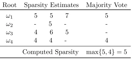
In contrast to the symbolic case, a majority is not guaranteed in the numeric case, because the numeric algorithm can under- and even overestimate tdue to unlucky randomization and noise, respectively. Similarly, wrong majorities may arise. In the cases where a majority does not exist, segments with outliers are indistinguishable from faulty noisy ones, so the algorithm returns FAIL if there is no majority for any root of unity. A hypothetical example of Majority Rule with four roots of unity and E = 1 (i.e., three segments per root) is shown in Table 1

below.

Table 1: Majority Rule example Root Sparsity Estimates Majority Vote

ω1 5 5 7 5

ω2 - 5 -

-ω3 4 6 5

-ω4 4 4 - 4

(32)

When substantial/unlucky noise does interfere, we still may be able to recover some accurate information. For example, given the 10-term Laurent polynomial

f = 48x32+ 24x25−53x22+ 67x−1−69x−7−5x−10−63x−16−37x−28−25x−35+ 16x−43

withDlow=−100,D= 100,T = 15, a noise scaling factor of 10−7, ill-conditionedness threshold

of 103, and three random roots of unity, a particular randomization (of random floating point noise distribution and choice of roots of unity) yields an interpolantf9 that has only nine terms

and is a poor fit to the noisy evaluations (compared to f itself). However, the nine exponents off9 are found in f, andkf9k2 has a relative error (with respect tokfk2, ignoring the dropped

monomial) of 0.036.

Another randomization yields an interpolant f10 that has ten terms and is a slightlybetter

fit to the noisy data than f itself; in this case, kf10k2 has a relative error (with respect to

kfk2) on the order of 10−7. Yet another randomization yields an interpolantf11that has eleven

terms and is also a slightly better fit to the noisy data than f itself, though a worse fit than f10. However, kf11k2 has a smaller relative error (with respect to kfk2, ignoring the extra

monomial) thankf10k, which suggests that the behavior of the noise is partially encoded in the

extra monomial off11, where the coefficient has absolute value on the order of 10−6.

2.7 Future Work

Our problem formulation, smoothing over incorrect values during the process of sparse recon-struction, applies to all such inverse problems, e.g., supersparse polynomial interpolation [Garg and Schost 2009] and [Kaltofen 2010, Section 2.1], computing the sparsest shift [Grigoriev and Karpinski 1993;Giesbrecht, Kaltofen, and Lee 2003] and the supersparsest shift [Giesbrecht and Roche 2010], or the more difficult exact and numeric sparse and supersparse rational function recovery [Kaltofen, Yang, and Zhi 2007;Kaltofen and Nehring 2011]. Our methods immediately apply to algorithms that are based on computing a linear recurrence, such as the supersparse interpolation algorithms in [Kaltofen 2010] and [Garg and Schost 2009]. The former needs no modification, and for the latter, one uses the majority rule algorithm for the sparse recovery with errors of the modular images f(x) mod (xp₋_{1), where}_p _{is chosen sufficiently large (and} random). The sparse interpolation with errors is at ω = (xrmod (xp−1+· · ·+ 1)), where r is random for early termination. One may assume that some polynomial residues f(ωi_{) mod} (xp−1 ₊ _{· · ·} _{+ 1) are faulty. The Chinese remaindering of the term exponents with several}

(33)

Algorithms for the supersparsest shift and sparse and supersparse rational function recovery with outliers in the values are subjects of current research.

(34)

Note 2. The following modifications have been made from [Comer, Kaltofen, and Pernet 2012]. 1. Page 7: “interpolations algorithms” has been changed to “interpolation algorithms”. 2. Page 9: “is Ben-Or/Tiwari’s” has been changed to “is Ben-Or’s/Tiwari’s”.

3. Page 12: the citation in the proof of Theorem2 has been updated.

4. Page 13: “Berlekamp-Massey” has been changed to “Berlekamp/Massey”.

5. Page 14: “and the second guaranties” has been changed to “and the second guarantees”. 6. Algorithms1,2,3, and4 have been reformatted.

7. The input (c0, . . . , cn−1) of Algorithm3 has been changed to (a0, . . . , an−1).

8. Page 16: “are error-free” has been changed to “is error-free”.

9. Page 17: “errors in a t of ” has been changed to “errors in a sequence of”

10. Page17: “generator of degreet,e+ 1 ‘blocks’ ” has been changed to “generator of degree t, thene+ 1 ‘blocks’ ”.

11. The title of Section2.5.1has been changed.

12. Page 18: “with bands given by” has been changed to “generated by”. 13. The title of Section2.6has been changed.

14. Note1 has been added.

(35)

Chapter Three

Sparse Polynomial Interpolation

by Variable Shift

This chapter is [Boyer, Comer, and Kaltofen 2012], except for the modifications listed in Note3.

3.1 Introduction

(36)

and rational function recovery via Zippel’s variable-by-variable sparse interpolation [Kaltofen, Yang, and Zhi 2007].

Already in the beginning days of symbolic computation, the choice of polynomial basis was recognized: (x−2)100+ 1 is a concise representation of a polynomial with 101 terms in power basis representation. The discrete-continuous optimization problem of computing the sparsest shift of an exact univariate polynomial surprisingly has a polynomial-time solution [Grigoriev and Karpinski 1993;Grigoriev and Lakshman 2000; Giesbrecht, Kaltofen, and Lee 2003]. Our subject is the computation of an approximate interpolant that is sparsified through a shift. One can interpret our algorithm as a numerical version of the exact sparsest shift algorithms. As in least squares fitting, noise can be controlled by oversampling (cf. [Giesbrecht and Roche 2011]). The main difficulty is that the shift is unknown. Our numerical algorithm adapts Algorithm UniSparsestShiftshone proj, two seqiin [Giesbrecht, Kaltofen, and Lee 2003] to compute the shift: UniSparsestShiftshone proj, two seqi carries the shift as a symbolic variable z throughout the sparse interpolation algorithm. Since the coefficients of the polynomials in the shift variable zare spoiled by noise, the GCD step becomes an approximate polynomial GCD. A main question answered here is whether the arising non-linear optimization problems remain well-conditioned. Our answer is a conditional yes: an optimal approximate shift is found among the arguments of all local minima, but the number of local minima is high, preventing the application of standard approximate GCD algorithms. Instead, we perform global optimization, as a fallback, by computing all zeros of the gradient ideal. In addition, our algorithm requires high precision floating point arithmetic.

In [Comer, Kaltofen, and Pernet 2012], we have introduced outlier values to the sparse inter-polation problem. There, outlier removal requires high oversampling, as the worst case ofk-error linear complexity is 2t(2k+ 1), wheretis the generator degree. However, ours is only an upper bound for sparse interpolation. The situation is different for AlgorithmUniSparsestShiftshone proj, two seqi. Outliers can be removed at the construction stage of the values containing the shift variablez, by a numeric version of Blahut’s decoding algorithm for interpolation with errors. The algorithm, numerical interpolation with outliers, is interesting in its own right. As we will show in Section3.3, the analysis in [Giesbrecht, Labahn, and Lee 2009;Comer, Kaltofen, and Pernet 2012] does not directly apply, as randomization can only be applied with a limited choice of random evaluation points. We have successfully tested it as a subroutine of our nu-merical sparsest shift algorithm. Note that a few outliers per interpolation lead to a very small sparse interpolation problem for error location, which can be handled successfully by sparse interpolation with noisy values.

(37)

with a weighted least squares fit for removing outliers and tolerating noise, we manage to compare favorably to the main algorithm.

In Section 3.4, we present the preliminary experimental results that our algorithms can recover sparse models even in the presence of substantial noise and outliers. See Section 3.4.3

for our conclusions.

3.2 Computing Sparse Shifts

We introduce in this subsection an algorithm to compute a shifted sparse interpolant in a numerical setting. The exact algorithm accepts outliers and uses early termination; we adapt it to a numerical setting, considering noisy and erroneous data. It is based on a numerical version of Blahut’s decoding algorithm.

3.2.1 Main Algorithm with Early Termination.

The Early Termination Theorem in [Kaltofen and Lee 2003] is at the heart of computing a sparsest shift. Let

g(x) = t

X

j=1

cjxej_, _cj _{6= 0 for all 1}_≤_j_≤_t,

be a t-sparse polynomial with coefficients in an integral domainD. Furthermore, let

αi(y) =g(yi)∈D[y], fori= 1,2, . . .

be evaluations ofg at powers of an indeterminate y. Prony’s/Blahut’s theorem states that the sequence of theαi is linearly generated by

Qt

j=1(λ−yej). Therefore, if one considers the Hankel

matrices

Hi(y) =

      

α1 α2 . . . αi

α2 α3 . . . αi+1

..

. ... . .. ... αi αi+1 . . . α2i−1

      

∈D[y]i×i_, _for_i_{= 1,}_{2, . . .}

one must have det(Ht+1) = 0. Theorem 4 in [Kaltofen and Lee 2003] simply states that

det(Hi) 6= 0 for all 1 ≤ i ≤ t. One can replace the indeterminate y by a randomly sam-pled coefficient domain element to have det(Hi) 6= 0 for all 1 ≤ i ≤ t with high probability (w.h.p.).

Error Correction for Symbolic and Hybrid Symbolic-Numeric Sparse Interpolation Algorithms.

Abstract

Dedication

Biography

Acknowledgements

Table of Contents

List of Tables

List of Figures

Chapter One

Introduction

Chapter Two

Sparse Polynomial Interpolation

with Noise and Outliers (

SPINO

)

2.1

Introduction

2.2

Length Bounds for Computing Linear Generators From

Se-quences with Error

2.3

Reed-Solomon decoding

2.4

A Fault-Tolerant Berlekamp/Massey algorithm

2.5

The Majority Rule Berlekamp/Massey algorithm

2.6

Implementation and Experiments of

SPINO

2.7

Future Work

Chapter Three

Sparse Polynomial Interpolation

by Variable Shift

3.1

Introduction

3.2

Computing Sparse Shifts