University of Windsor University of Windsor
Scholarship at UWindsor
Scholarship at UWindsor
Electronic Theses and Dissertations Theses, Dissertations, and Major Papers
2019
A Voting Algorithm for Dynamic Object Identification and Pose
A Voting Algorithm for Dynamic Object Identification and Pose
Estimation
Estimation
Chandini Ravindranathan Nair University of Windsor
Follow this and additional works at: https://scholar.uwindsor.ca/etd
Recommended Citation Recommended Citation
Nair, Chandini Ravindranathan, "A Voting Algorithm for Dynamic Object Identification and Pose Estimation" (2019). Electronic Theses and Dissertations. 7724.
https://scholar.uwindsor.ca/etd/7724
This online database contains the full-text of PhD dissertations and Masters’ theses of University of Windsor students from 1954 forward. These documents are made available for personal study and research purposes only, in accordance with the Canadian Copyright Act and the Creative Commons license—CC BY-NC-ND (Attribution, Non-Commercial, No Derivative Works). Under this license, works must always be attributed to the copyright holder (original author), cannot be used for any commercial purposes, and may not be altered. Any other use would require the permission of the copyright holder. Students may inquire about withdrawing their dissertation and/or thesis from this database. For additional inquiries, please contact the repository administrator via email
A Voting Algorithm for Dynamic Object Identification and Pose Estimation
byCHANDINI RAVINDRANATHAN NAIR
A THESIS
Submitted to the Faculty of Graduate Studies Through Computer Science
In Partial Fulfilment of the Requirements for The Degree of Master of Science at the
University of Windsor
Windsor, Ontario, Canada 2019
A Voting Algorithm for Dynamic Object Identification and Pose Estimation
byChandini Ravindranathan Nair
APPROVED BY:
_______________________________________ G.Lan
Odette School of Business
_______________________________________ A.Ngom
School of Computer Science
_______________________________________ X.Yuan, Advisor
School of Computer Science
iii
Declaration of Originality
I confirm here that I am the sole creator of this thesis and no piece of this proposition has been
distributed or submitted for production.
I affirm to the best of my insight, my proposition does not encroach upon anybody's copyright nor
damage any restrictive rights and their thoughts, methods, citations, or some other material crafted
by other individuals incorporated into my postulation, circulation or something else, and are
entirely recognized as per the standard referencing hone. Moreover, I have included copyrighted
material that outperforms the limits of reasonable managing inside the significance of the Canada
Copyright Act. I affirm to acquire a composed consent from the copyright owner(s) to incorporate
such material(s) in my postulation and have included duplicates of such copyright clearances in
my reference section.
I pronounce this is a genuine copy of my thesis including any last updates, as affirmed by my thesis
advisory group and the Graduate Studies office, and this theory has not been submitted for a higher
iv
Abstract
While object identification enables autonomous vehicles to detect and recognize objects from
real-time images, pose estimation further enhances their capability of navigating in a dynamically
changing environment. This thesis proposes an approach which makes use of keypoint features
from 3D object models for recognition and pose estimation of dynamic objects in the context of
self-driving vehicles. A voting technique is developed to vote out a suitable model from the
repository of 3D models that offers the best match with the dynamic objects in the input image.
The matching is done based on the identified keypoints on the image and the keypoints
corresponding to each template model stored in the repository. A confidence score value is then
assigned to measure the confidence with which the system can confirm the presence of the matched
object in the input image. Being dynamic objects with complex structure, human models in the
"COCO-DensePose" dataset, along with the DensePose deep-learning model developed by the
Facebook research team, have been adopted and integrated into the system for 3D pose estimation
of pedestrians on the road. Additionally, object tracking is performed to find the speed and location
details for each of the recognized dynamic objects from consecutive image frames of the input
video. This research demonstrates with experimental results that the use of 3D object models
enhances the confidence of recognition and pose estimation of dynamic objects in the real-time
input image. The 3D pose information of the recognized dynamic objects along with their
corresponding speed and location information would help the autonomous navigation system of
the self-driving cars to take appropriate navigation decisions, thus ensuring smooth and safe
v
Dedication
I dedicate this thesis work to God Almighty, my dear husband Mr. Navaneeth Narayanan, my
beloved parents Mr. Ravindranathan Nair and Mrs. Hemalatha R Nair, my loving brother Mr.
vi
Acknowledgements
First and foremost, I would like to express profound thankfulness to my supervisor, Dr. Xiaobu Yuan, who has supported me throughout my thesis with his knowledge and expertise on this
exciting field of research. His ideas and suggestions have helped me become more creative, without which I would not have been able to complete this research.
I would like to offer my sincere gratitude to the advisory group members, Dr. Alioune Ngom and
Dr. George Lan for their significant remarks and recommendations for my research.
I want to thank, my friend, Mr. Jonathan Ketel, Full Stack Developer, UNI3T, Montreal, for proof
reading this thesis book and providing his valuable suggestions.
I would like to thank all my friends, who have supported and helped me throughout my studies, here in Canada. I also thank my parents, husband and family for their blessings and financial
vii
Table of Contents
Declaration of Originality ... iii
Abstract ... iv
Dedication ... v
Acknowledgements ... vi
List of Figures ... ix
List of Abbreviations/Symbols ... xii
List of Tables ...xiii
Chapter 1: Introduction ... 1
1.1 Google’s Self Driving Car ... 3
1.2 Object Recognition – How do self-driving cars see? ... 4
1.3 Pose Estimation ... 5
Chapter 2: Literature Review ... 6
2.1 Object Recognition and Pose Estimation of Objects ... 6
2.2 Semantic Segmentation Techniques ... 8
2.2.1 Region Based Semantic Segmentation ... 10
2.2.2 Fully Convolutional Network Based Semantic Segmentation ... 13
2.2.3 Weakly Supervised Semantic Segmentation ... 13
2.3 Object Detection via Bounding Boxes ... 14
2.4 3D Object Recognition... 15
2.5 Object Recognition and Pose Estimation of Cars using 3D Models ... 24
2.6 Object Recognition and Pose Estimation of Humans using 3D Models ... 31
2.7 Related Works ... 39
2.8 Thesis Statement ... 49
2.8.1 Problem Statement ... 49
2.8.2 Thesis Contribution ... 49
Chapter 3: Proposed System ... 52
3.1 Motivation ... 52
3.2 Relation of the thesis to other components of the overall system ... 53
3.2.1 Modules of the overall system directly related to the thesis research ... 55
3.3 Proposed Techniques for Dynamic Object Recognition and Pose Estimation ... 57
viii
3.3.2 Object Recognition and Pose Estimation of Humans ... 62
3.4 Proposed Technique for Dynamic Object Tracking ... 64
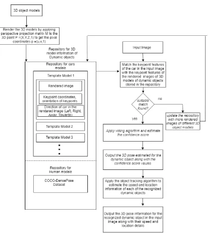
3.5 Design of the Flowchart and Algorithms ... 67
3.5.1 The Proposed Algorithm for Recognition, Pose Estimation and Tracking of Dynamic Objects in the Real-Time Input Image ... 70
3.5.2 The Proposed Voting Algorithm for Cars ... 71
3.5.3 The Proposed Object Tracking Algorithm ... 74
3.6 Time Complexity of the Proposed Algorithm ... 75
Chapter 4: Implementation and Experiments ... 77
4.1 Software Information ... 77
4.2 Experiments and Results of Object Recognition and Pose Estimation of Cars ... 78
4.2.1 Simulated input image with a single car ... 78
4.2.2 Real-time input image with a single car ... 84
4.2.3 Real-time input image with a car partially occluded by another car ... 88
4.2.4 Real-time input image with part of the vehicle missing... 90
4.2.5 Real-time input image with objects other than cars or pedestrians ... 92
4.3 Experiments and Results of Object Recognition and Pose Estimation of Pedestrians ... 93
4.3.1 Input image with an adult on the road ... 93
4.3.2 Input image with an adult and child on the road ... 95
4.3.3 Real-time input image with pedestrians running across the road ... 97
4.3.4 Real-time input image with multiple people on road (Occluded humans) ... 98
4.4 Results of the Tracking of Dynamic Objects ... 100
4.5 Comparison and Discussions ... 102
4.5.1 Mean Average Precision ... 102
4.5.2 Estimation of Mean Average Precision using the proposed method ... 103
4.5.3 Results Comparison and Discussion: Cars ... 105
4.5.4 Results Comparison and Discussion: Humans ... 108
4.6 Observation and Limitations ... 110
Chapter 5: Conclusion and Future Work ... 112
References ... 114
ix
List of Figures
Figure 1: Google’s Self-Driving Car prototype ... 4
Figure 2: Object recognition to identify different objects ... 6
Figure 3: Pose estimation in humans and cars ... 7
Figure 4: Object recognition in the context of autonomous cars ... 8
Figure 5: Semantic segmentation of objects on the road ... 9
Figure 6: The architecture of R-CNN (Image source: Girshick et al., 2014) ... 10
Figure 7: The architecture of Fast R-CNN. (Image source: Girshick, 2015) ... 11
Figure 8: An illustration of Faster R-CNN model. (Image source: Ren et al.,2016) ... 12
Figure 9: FCN Architecture ... 13
Figure 10: Weakly supervised semantic segmentation ... 14
Figure 11: Illustration of YOLO ... 15
Figure 12: Illustration of strategy suggested by Schmid and Mohr ... 19
Figure 13: A general 3D object recognition system... 21
Figure 14: Graphical representation of SIFT algorithm ... 22
Figure 15: Process for Bag of Features Image Representation ... 23
Figure 16: Sample 3D car model (.obj) ... 24
Figure 17: Image Formation: Pinhole model (Perspective model) ... 25
Figure 18: Different views of 3D car model ... 26
Figure 19: Rendered images of 3D car models ... 27
Figure 20: Training and Inference stages of KeypointNet ... 28
Figure 21: SMPL model (orange) fit to ground truth 3D meshes (gray) ... 32
Figure 22: Representation of Standard Skinning ... 33
Figure 23: SMPL Model Pipeline ... 34
Figure 24: Part segmentation, Marking Correspondences and Surface Correspondence illustrative representation ... 35
Figure 25: Left: The image and the regressed correspondence by DensePose-RCNN, Middle: DensePose COCO Dataset annotations, Right: Partitioning and UV parametrization of the body surface ... 36
Figure 26: The user interface for collecting per-part correspondence annotations ... 36
Figure 27: The classification and regression steps of DensePose architecture ... 37
Figure 28: DensePose R-CNN architecture ... 38
Figure 29: Cross-cascading architecture ... 39
Figure 30: Flowchart of the overall system ... 53
Figure 31: Snippet of the repository ... 58
Figure 32: Object center candidates ... 60
Figure 33: Flowchart representing the proposed technique for object recognition and pose estimation of dynamic objects ... 68
Figure 34: Flowchart depicting the proposed technique for object tracking from input video ... 69
Figure 35: Input image ... 78
Figure 36: Keypoints detected using KeypointNet ... 79
Figure 37: Matched model from the repository ... 80
Figure 38: Image centre coordinates ... 80
x
Figure 40: Representation of results in each step... 81
Figure 41: Car detected with confidence score = 1.0 ... 82
Figure 42: Step-wise results for the image of a car moving in the "Towards" direction ... 83
Figure 43: Step-wise results for the image of a car moving in the "Left" direction ... 83
Figure 44: A real time road scene with a single car ... 84
Figure 45: Cropping the detected car using ImageAI python library ... 85
Figure 46: Keypoint features identified using KeypointNet ... 85
Figure 47: Matched model from the repository ... 86
Figure 48: Object centre and object centre candidates ... 86
Figure 49: Step-wise representation of results for real time single car scenario ... 87
Figure 50: Car detected with confidence score = 1.0 in real time image ... 87
Figure 51: Real time road scene with multiple cars ... 88
Figure 52: Cars Detected and cropped using the ImageAI library and the Resnet model ... 89
Figure 53: Step-wise results for the image of a car partly occluded by the tyre of another car ... 89
Figure 54: Tractor unit without a trailer on the road ... 90
Figure 55: Step-wise results for vehicle with a missing part ... 91
Figure 56: Input images with no car or pedestrians ... 92
Figure 57: Keypoint features detected on images without cars or pedestrians ... 92
Figure 58: Input image with an adult on the road ... 94
Figure 59: Visualization of the isocontours of the UV fields in the image with an adult on the road ... 94
Figure 60: Textures mapped on the isocontours of the UV fields in an image with an adult on the road .. 95
Figure 61: Input image with an adult and a child crossing the road ... 95
Figure 62: Visualization of the isocontours of the UV fields in the image with an adult and a child crossing the road ... 96
Figure 63: Textures mapped on the isocontours of the UV fields for an image with an adult and a child crossing the road ... 96
Figure 64: Input image with two men running across the road ... 97
Figure 65: Visualization of the isocontours of the UV fields in an image with two men running across the road ... 97
Figure 66: Textures mapped on the isocontours of the UV fields for an image with two men running across the road... 98
Figure 67: Input image with multiple pedestrians (few partly occluded) crossing the road ... 98
Figure 68:Visualization of the isocontours of the UV fields in the image with multiple pedestrians (few partly occluded) crossing the road ... 99
Figure 69: Textures mapped on the isocontours of the UV fields for an image with multiple pedestrians (few partly occluded) crossing the road ... 99
Figure 70: Different frames of the input video tracking the car with the estimated speeds displayed on it ... 100
Figure 71: Different frames of the input video tracking the humans with the estimated speeds displayed on it ... 101
Figure 72: Object recognition with Resnet model ... 106
Figure 73: Pictorial representation of how the proposed approach improves prediction confidence ... 107
Figure 74: Step-wise representation of results for input image of car with partial occlusion ... 107
Figure 75: Objects detected incorrectly instead of cars (Source: Tangruamsub et al.,2011) ... 108
xi
Figure 77: Pose estimation results after applying DensePose model ... 110
Figure 78: Two cars in two opposite directions with keypoints at similar coordinate positions ... 111
xii
List of Abbreviations/Symbols
HPE Human Pose Estimation
CNN Convolutional Neural Network
R-CNN Region Based Convolutional Neural Network
SMPL Skinned Multi-Person Linear Model
YOLO You Only Load Once
SURREAL Synthetic hUmans foR REAL tasks
LiDAR Light Detection and Ranging
ROI Region of Interest
FCN Fully Convolutional Network
SIFT Scale Invariant Feature Transformation
SOA Service Oriented Architecture
xiii
List of Tables
Table 1: Review of object recognition and pose estimation methods ... 44
Table 2: Time complexity of the algorithm ... 76
Table 3: List of tools used for implementation of the proposed system ... 77
Table 4: Confusion Matrix ... 103
1
Chapter 1: Introduction
Human society is moving towards a future where cars will be able to drive by themselves and
travelers can just sit back and relax. Apart from the major players like Tesla, Google and Uber, there are many other companies who have invested billions of dollars towards research in this area to make the dream of a fully autonomous car a reality. With so much investment and interest in
driverless technology, it is easy to assume that self-operating cars are imminent, but they are still far from being viable. Creation of such a sophisticated machine requires great expertise to ensure
smooth and safe driving. Object recognition and pose estimation of recognized objects are the two most important tasks in the application of vehicle surveillance [91]. An accurate solution to these problems will help with automatically analyzing a traffic scene. This includes the analysis of
crucial information for vehicle navigation like determining the vehicle speed, traffic frequency, driver behaviour, or the shape and style of traffic participants. It is a known fact that there would
be a variety of objects on the road at any given time. These objects can be either moving or stationary objects. In the context of self-driving vehicles, it is important to distinguish between the moving and stationary objects in order to take the correct navigation decisions. Kolski et al. [74]
describes the objects like pedestrians and other vehicles which move on the road as dynamic obstacles. Darms et al. [75] clearly defines static obstacles as objects which are assumed not to
move during the observation period, such as, buildings, traffic cones or parked cars which do not participate actively in traffic. In contrast, Darms et al. [75] define dynamic obstacles as objects which potentially move during the observation periods. Darms et al. [76] and Hu et al. [77]
categorize the moving objects as "dynamic objects" and the objects which do not move as "static objects" in their works. Hu et al. [77] include blockages such as stones and construction signs into
2
estimation of moving objects like cars and pedestrians, on the road. More formally, this thesis
deals with object recognition and pose estimation of “dynamic objects” on the road.
A system with very high obstacle detection accuracy is required for a self-driving car, as lower
accuracies can lead to errors which can be dangerous and cost human lives [78]. Most of the previous researches [1, 28, 84] use the mean average precision(mAP) (Section 4.5.1) as the
measure of the accuracy in the object detection and pose estimation predictions. For example, the current state-of-the-art technique YOLOv2 has achieved a mAP of 78.6 [28]. Janai et al. [81] discuss the importance of reliable object detection in the context of self-driving vehicles, in order
to avoid accidents that might be life-threatening. The work also discusses the difficulties in object detection due to the wide variety of object appearances and occlusions caused by other objects. Gao et al. [79] mention the bottlenecks in accuracy, efficiency, and timeliness of detection,
recognition, tracking, and segmentation techniques based on traditional RGB images due to insufficient depth information. Gene Lewis [80] discusses the challenges in the object detection
problem ported to the self-driving vehicles, such as the optimization problems and the speed issues of the object detection pipeline. Hence, even though 100% accuracy is almost impossible, there is a need for continuous improvement in the confidence level with which an object is identified, until
it is safe to put self-driving vehicles on the road.
The aim of this research is to improve the confidence with which the system can confirm the
presence of an object or obstacle at a location in the input image. An object is identified, and its 3D pose is determined by making use of keypoint information from the 3D object models. A voting
3
object in the input image. The term “voting” was adopted for this algorithm from a similar work
done by Tangruamsub et al. [1], where the authors used keypoint features from 2D images (instead of 3D models used in this thesis) to vote out the best candidates for object recognition and pose
estimation. The identified object is then tracked to get its speed and location information. The estimated pose information along with the speed and location information is then used to update the recognized dynamic object on to a virtual city which acts as a repository of both the static and
dynamic objects on the road in real-time.
1.1Google’s Self Driving Car
Many companies like Tesla, Mercedes, Uber, Google, BMW, and Volvo already have their semi-autonomous cars on the market. However, all of these require expensive hardware support and are
still far from being fully autonomous vehicles. Among them is Google’s Self Driving Car. Google was the first company to make customer oriented driverless cars, but it is still far from viability. The car uses many highly advanced pieces of hardware for obstacle detection and therefore the
overall cost of the vehicle is a major problem. However, this cannot be avoided as the vehicle needs to be able to detect and avoid obstacles like other cars, pedestrians, cyclists and animals. Google’s Self-Driving Car uses an array of detection technologies including sonar devices, stereo
cameras, lasers, and radar. The LiDAR on top of the car is considered the heart of object detection. Google’s LiDAR system is great for generating an accurate map of the area surrounding the
vehicle, but it is not ideal for monitoring the speed of other cars in real time. Therefore, the front and back bumper of the driverless car include radar. Hence, it is clear that many expensive
4
Figure 1: Google’s Self-Driving Car prototype
1.2Object Recognition – How do self-driving cars see?
In addition to reducing human effort on the road, it is anticipated that self-driving cars will make driving safer and therefore reduce the number of traffic accidents and fatalities. This will require these vehicles to have highly accurate object recognition techniques. A large amount of machine
learning and computer vision research is currently focused on this area. Basically, there are two categories of object recognition in the context of autonomous driving: - Semantic Segmentation
and Object Detection using rectangular bounding boxes [11]. However, these methods are mostly done with 2D images. The novel idea used by the proposed system of this research makes use of the keypoint feature information from 3D object models to identify the dynamic objects from a
5 1.3Pose Estimation
In the context of self-driving vehicles, the pose estimation of objects on the road is very significant in the autonomous navigation of the vehicle [12]. Pose estimation of recognized objects can be classified into two:
a. Pose estimation of objects which do not change its structure significantly. b. Pose estimation of objects whose structure may change.
Examples of objects whose structure does not significantly change include vehicles such as cars and trucks. Whereas examples of objects whose structure does change significantly include people, animals, and birds. This research also focuses on the pose estimation of identified objects on the
road, which will provide additional information for the autonomous navigation systems of the self-driving vehicles, to take good navigation decisions.
In this thesis, Chapter 2 contains a detailed review of the previous work done on object recognition and pose estimation in autonomous vehicles. It also includes the prerequisite techniques for the proposed approach. Chapter 3 explains the proposed system in depth. Chapter 4 discusses the
different scenarios that were considered during the implementation of the proposed idea along with the results obtained. Chapter 4 also compares and discusses the results obtained using the proposed
6
Chapter 2: Literature Review
This chapter discusses the relevant background of recent works in object recognition and pose
estimation in the context of self-driving vehicles. This section also covers the technical background of object recognition and pose estimation using 2D and 3D images and how it can be extended with the proposed approach of using 3D object models to improve object recognition and pose
estimation tasks.
2.1Object Recognition and Pose Estimation of Objects
Object recognition is a computer vision technique that identifies objects in images or videos. Humans can easily spot people, objects, and other visual details when they view a photograph or
watch a video. The goal of machine learning is to teach a computer to do what comes naturally to humans, specifically to gain a level of understanding of what objects an image contains. Figure 2 below shows an illustration of using an object recognition algorithm to identify if an object is a cat
or a dog [11].
7
Object recognition is one of the most important technologies used in autonomous vehicle
navigation. It allows the recognition of vehicles and pedestrians on the road or other objects such as a lamppost or a stop sign.
Pose estimation is a general problem in computer vision where the position and orientation of an object are detected [12]. It detects the keypoint locations that describe the object. Many prior works
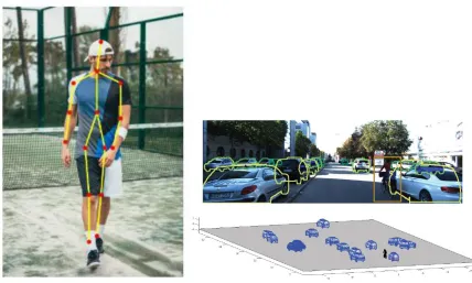
have been done on pose estimation of objects having skeletal structures such as humans, birds or animals, as well as on objects whose structure does not significantly change like that of cars. Figure 3 below depicts pose estimation in humans and cars [12].
Figure 3: Pose estimation in humans and cars
8
to make driving safer and reduce the number of road accidents. This motive requires that these
cars need exemplary object recognition techniques. Plenty of different machine learning and computer vision researches are happening in this area every day.
Figure 4: Object recognition in the context of autonomous cars
There are two major categories of object recognition in the context of autonomous driving:
a. Semantic Segmentation Technique b. Object Detection via bounding boxes
The different approaches adopted so far in both the categories are discussed in detail in the below sections.
2.2Semantic Segmentation Techniques
The semantic segmentation technique is understanding an image at the pixel level. In semantic
9
Many of the existing advanced deep learning networks for self-driving vehicles are based on
semantic segmentation and objects are detected based on edge detection. Also, many pieces of research like the works done by Teichmann et al. [14] and Ros et al. [15] deal with autonomous
driving technology based on the semantic segmentation technique.
Figure 5: Semantic segmentation of objects on the road
Some standard deep networks which are used as the basis of semantic segmentation systems are
AlexNet (Krizhevsky et al. [15]), VGG-16 (Simonyan et al. [16]), GooLeNet (Szegedy1 et al. [17]), ResNet (He et al. [18]).
Basically, a semantic segmentation architecture can be broadly considered as an encoder
followed by a decoder.
There are three main approaches which are currently adopted:
a. Region Based Semantic Segmentation
10 2.2.1 Region Based Semantic Segmentation
The region-based methods generally follow the “segmentation using recognition” pipeline, which first extracts free-form regions from an image and describes them, followed by region-based classification. There are three main region based deep learning segmentation approaches which
were once state-of-the-art before the YOLO: R-CNN, Fast R-CNN and Faster R-CNN.
2014: R-CNN – An early application of CNN to object detection – The goal of R-CNN is to take
an image, and then correctly identify where the specific objects are within that image. The main idea of R-CNN is composed of two steps. First, using selective search, it extracts about 2000 regions from the image. These are called the region proposals.
Figure 6: The architecture of R-CNN (Image source: Girshick et al., 2014)
These region proposals are wrapped into a square and fed into a convolutional neural network that
produces a 4096-dimensional feature vector as output. The convolutional neural network acts as a feature extractor and the output dense layer consists of features extracted from the image. These extracted features are then fed into a support vector machine, to classify the object present within
that candidate region proposal. However, the R-CNN has some issues. The training time of the network is very high, as 2000 region proposals per image need to be classified. It is not easy to
11
since the selective search algorithm is a fixed algorithm, no learning happens at that stage. This
could lead to bad candidate region proposals.
2015: Fast R-CNN – Speeding up and Simplifying R-CNN – In Fast R-CNN instead of feeding
the region proposals to the CNN, the input image is fed to the CNN to generate a convolutional feature map. The region of proposals is identified from the convolutional feature map and are then
wrapped into squares.
Figure 7: The architecture of Fast R-CNN. (Image source: Girshick, 2015)
By using a RoI pooling layer, it is reshaped into a fixed size so that it can be fed into a fully connected layer. From the RoI feature vector, a softmax layer is used to predict the class of the
proposed region and the offset values for the bounding box. Fast R-CNN is faster than R-CNN as there is no need to feed the 2000 region proposals to the convolutional neural network every time.
12
2016: Faster R-CNN – Speeding up Region Proposal
Both R-CNN and Fast R-CNN uses selective search to find out the region proposals, which is a slow and time-consuming process affecting the performance of the network. Faster R-CNN is an
object detection algorithm that eliminates the selective search algorithm and lets the network learn the region proposals. Just like the approach in Fast R-CNN, the image is provided as an input to
the convolutional network which provides a convolutional feature map.
Figure 8: An illustration of Faster R-CNN model. (Image source: Ren et al.,2016)
Instead of using the selective search algorithm on the feature map to identify the region proposals,
13 2.2.2 Fully Convolutional Network Based Semantic Segmentation
The original Fully Convolutional Network (FCN) learns the mapping from pixels to pixels, without extracting the region proposals. The main idea of FCN is to make the classical CNN take arbitrary-sized images as input. CNNs have fixed fully connected layers which restricts them to accept and
produce labels for specifically sized inputs only. However, the FCNs have only convolutional and pooling layers which give them the ability to make predictions on arbitrary-sized inputs. Figure 9
below shows the FCN architecture [46].
Figure 9: FCN Architecture
2.2.3 Weakly Supervised Semantic Segmentation
Most of the relevant methods in semantic segmentation rely on many images with pixel-wise
14
Figure 10: Weakly supervised semantic segmentation
2.3Object Detection via Bounding Boxes
This technique bounds the location of an object in the frame with a rectangular box. There are many high performing object detection models which detect multiple objects in a scene
simultaneously in a very short time. The bounding boxes are a simpler way to describe the location of an object when compared to the segmentation technique. The CNNs could usually only classify
images with a single object that take a sizable portion of it. This issue was solved using the sliding window approach. However, to identify the different object with various sizes, multiple window sizes are required which needs to be slide over the image. However, this is computationally very
expensive and hence the YOLO was introduced. In case of the YOLO network, the image is split up into a grid and the entire image is run through a convolutional neural network.
YOLO – You Only Load Once
You only load once (YOLO) is a state-of-the-art, real-time object detection system. YOLO applies
15
by the predicted probabilities. One of the advantages of YOLO is that it looks at the whole image
during the test time. Unlike R-CNN, which requires thousands of networks for a single image, YOLO makes predictions with a single network. This makes the algorithm extremely fast, over
1000 times faster than R-CNN and 100 times faster than Fast R-CNN. Figure 11 shows the illustration of the YOLO [28].
Figure 11: Illustration of YOLO
2.43D Object Recognition
With the increased availability of 3D data and the 3D sensors popularization, the 3D object
classification and recognition area have had a growing boost in the last few years. There are various applications for the methods developed in this area which range from the field of robotics, directed to robot movement in environments and object manipulation by robotic arms, to the security
16
vehicles which deals with lives of people on the road, it seemed to be a good idea to make use of
the 3D model information of the different objects on the road for recognizing them in the real-time images.
Object recognition is one of the basic application domains in computer vision. Extensive research has been and is still being done in this area, especially in 3D. 3D object recognition can be defined
as the task of finding and identifying objects in the real world from an image or a video sequence. Object recognition is still a hot research topic in computer vision because it has many challenges such as viewpoint variations, scaling, illumination changes, partial occlusion, and background
clutter. Many approaches and algorithms are proposed and implemented to overcome these challenges.
The object recognition research community can be split into two: Those who deal with 2D images
and those who deal with 3D point clouds or meshes. By projecting the scene onto a plane by capturing the light intensity detected at each pixel, the 2D images can be created. Alternatively,
3D point clouds capture the 3D coordinates of points in the scene. The main difference between two dimensional and three-dimensional data is that 3D data includes depth information whereas 2D data does not. Cheaper sensors have been developed to acquire the 3D data from the real
environments, such as RGB-D cameras. Mustafa et al. [47] and Krystof et al. [48] proposes works which make use of RGB-D cameras for object recognition. RGB-D cameras, such as the Microsoft
Kinect, capture a regular color image (RGB) along with the depth (D) associated with each pixel in the image. Since the approach is being applied to the self-driving vehicle domain, it is important
17
a) Evaluation Time: In most of the industrial applications, the data need to be processed in
real-time. In the case of self-driving vehicles, evaluation time is crucial to determine the correct navigation of the car in real time. The evaluation time depends strongly upon the
number of pixels covered by the object as well as the size of the image area to be examined. b) Accuracy: In the autonomous driving application, the object position needs to be determined very accurately. The error bounds cannot exceed more than a fraction of a pixel,
else it might result in disastrous events.
c) Recognition ability: In the scenario of autonomous driving, it is required that the rate of
false detection must be almost zero to ensure safe driving.
d) Invariance: In the autonomous driving scenario, it is worthwhile to achieve invariance with
respect to illumination, scale, rotation, background clutter, occlusion, and viewpoint changes.
The 3D object recognition techniques can be categorized into four groups: geometry-based
methods, appearance-based methods, three-dimensional object recognition schemes, and descriptor-based methods [29, 49,50,51,52]. In geometry- or model-based object recognition, the knowledge of an object's appearance is provided by the user as an explicit CAD-like model. Only
the 3D shape is described and properties such as color and texture are not included. In contrast, the Appearance-based methods do not require an explicit user-provided model for object
recognition. The object representations are usually acquired through an automatic learning phase, and the model typically relies on surface reflectance properties.
18
and the 3D keypoints are determined by selecting the feature points that are invariant to viewpoint
position. This explained in detail in the next section.
Geometry – or – model-based object recognition techniques have many advantages like invariance
to viewpoint and illumination. Also, they have a well-developed theory as many effective algorithms exist for analyzing and manipulating geometric structures. In contrast, most recent
research efforts have been centered on appearance-based techniques such as advanced feature descriptors and pattern recognition algorithms. They typically include two phases. In the first phase, from the set of reference images, a model is constructed. The set includes the appearance
of the object under different orientations, different illuminants and potentially multiple instances of a class of objects, for example, cars. In the second phase, parts of the input image (sub-images of the same size as the training images) are extracted, possibly by segmentation (by texture, color,
motion) or by exhaustive enumeration of image windows over the whole image. The recognition system then compares an extracted part of the input image with the reference images. However,
the major limitation of the appearance-based approaches is that they require isolation of the complete object of interest from the background and is hence sensitive to occlusion and require good segmentation.
The three-dimensional object recognition schemes are used by some applications that require a position estimate in 3D space and not just in the 2D image plane. Such systems make use of sensors
which generates 3D data and perform matching in 3D space. Another way to determine the 3D pose of an object is to estimate the projection of the object location in 3D space onto a 2D camera image. Such a data representation is not “full” 3D yet and therefore is often called 2.5D.
19
heavy background clutter and occlusion. Schmid and Mohr [53] suggested a two-way method for
image-content description. In the first step, the keypoints are detected, i.e. points that exhibit salient characteristic like the corner of a building. Subsequently, for each interest point, a feature
vector called region descriptor is calculated. Each region descriptor characterizes the image information available in a local neighborhood around one interest point. Figure 12 illustrates the strategy suggested by Schmid and Mohr [53].
Figure 12: Illustration of strategy suggested by Schmid and Mohr
Object recognition can then be performed by comparing the information of region descriptors detected in a scene image to the information of region descriptors in a model database. A similar
technique is being adopted in the proposed method. However, the proposed approach extracts keypoint features from the 3D object models and stores them in a repository.
The 3D data are obtained using different methods which makes use of extra hardware, for e.g.
sensors. Most of the semi-autonomous cars now in the market, use a variety of expensive sensors for this purpose. Cost is hence one of the drawbacks of the autonomous cars today. Stereo
20
approach for 3D mapping and object reconstruction using 2D images. Acquisition from acquired
sensor data is done using a variety of sensors, including stereo cameras, time of fight laser scanners such as LiDARs, as well as infrared sensors such as the Microsoft Kinect or Panasonic DI-Imager.
All these sensors can only capture a single view of the object with a single scan. This view is referred to as a 2½D scan of the object. Therefore, to capture the entire 3D shape of the object, the sensor captures multiple instances of the object from different viewpoints. The process of
determining the similarity between the scene object and the model stored in a repository is one of the important tasks in 3D object recognition. This is done by computing the distance between
feature vectors. In general, the recognition must search among the possible candidate features for identification of the best match and then assign the label to the matched object in the scene [54].
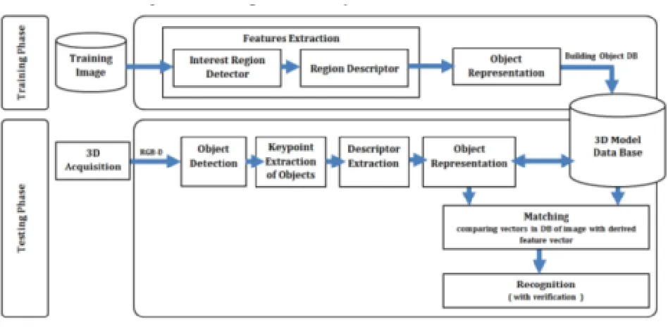
Based on the characteristics of the shape descriptor, the 3D object recognition methods can be divided into two main categories: global feature methods and local feature methods [54]. Figure 13 below shows a general 3D object recognition system [29]. Points from an image which gives
the best definition for an object are called the keypoint features and they are very important and valuable in applications of image processing like object detection, object and shape recognition,
21
Figure 13: A general 3D object recognition system
Some of the important feature extraction techniques are discussed briefly below:
A. Harris Corner Detector: Harris and Stephens [55] developed an approach to extract corners and infer the contents of an image. In the context of the autonomous vehicles, it requires
that the car recognizes static objects like buildings on the roadside. The detection of corner points of buildings will give more information regarding the pose and shape of the
buildings. A corner is so special because, as it is the intersection of two edges and represents a point in which the directions of these two edges change. The Harris corner detector is popular because it is independent of rotation, scale, and illumination variations.
B. The SIFT Algorithm: Lowe [56] developed a feature detection and description technique called SIFT (Scale Invariant Feature Transformation). The keypoints are extracted and
22
keypoints are described as 128 vectors. Finally, the last step is the matching stage. This is
depicted in Figure 14 below [29].
Figure 14: Graphical representation of SIFT algorithm
C. The SURF Algorithm: Bay et al. [57] developed the SURF Algorithm which is based on the SIFT algorithm [56]. It achieves higher speed than SIFT using integral images and
approximations. These integral images are used for convolution. Like SIFT, SURF also works in three main stages: extraction, description, and matching. The difference between
SIFT and SURF is that SURF extracts the features from an image using integral images and box filters.
D. The ORB Algorithm: The ORB algorithm has several advantages over the more established
vector-based descriptors such as SIFT and SURF. ORB [58] is scale and rotation invariant, robust to noise and affine transformations. The algorithm is a combination of the FAST
keypoint detection with oriented keypoints added to the algorithm.
23
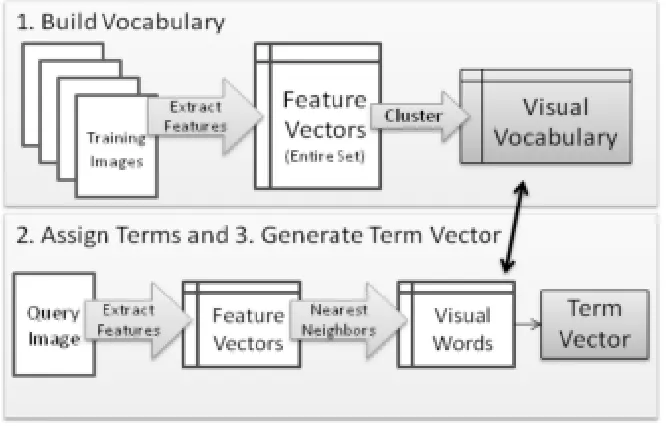
procedure for generating a Bag of Features image representation is illustrated in Fig 15 and
summarized as follows [59]:
1) Build Vocabulary: Extract features from all images in a training set. Vector quantize, or cluster, these features into a “visual vocabulary,” where each cluster represents a “visual
word” or “term.” In some works, the vocabulary is called the “visual codebook.” Terms in the vocabulary are the codes in the codebook.
2) Assign Terms: Extract features from a novel image. Use Nearest Neighbors or a related strategy to assign the features to the closest terms in the vocabulary.
3) Generate Term Vector: Record the counts of each term that appears in the image to create a normalized histogram representing a “term vector.” This term vector is the Bag of
Features representation of the image. Figure 15 below represents the Process for Bag of Features Image Representation [29].
24
All the previous works have done 3D object recognition from three different aspects: 3D object
recognition from range images, 3D local descriptors, and 3D object recognition based on stereo vision. The method proposed in this research aims to use similar keypoint feature extraction
technique followed by feature matching approach, using 3D object models. The KeypointNet [23] model is used for extracting the keypoint features from the 3D models after rendering it which serves as input to the proposed system which will be discussed in detail in Chapter 3.
2.5Object Recognition and Pose Estimation of Cars using 3D Models
The proposed system uses 3D models in the .obj file format for building up the input repository
with the keypoint features extracted from these models. Figure 16 below shows a sample 3D car model (.obj). The OBJ file extension is known as Wavefront 3D Object File which was developed
by Wavefront Technologies. The .obj is a file format used for a three-dimensional object containing 3D coordinates (polygon lines and points), texture maps, and another object information [61].
Figure 16: Sample 3D car model (.obj)
The .obj images need to be rendered to extract the optimal set of keypoints for recovering the
25 Rendering of the 3D model
The image formation is the process by which a 3D representation of a scene is reduced to a 2D representation of that same scene, an image.
3D scene → transformation → 2D image
Figure 17 below illustrates the Image Formation: Pinhole model [62].
Figure 17: Image Formation: Pinhole model (Perspective model)
An image point (pixel), given by its image coordinates, is the result of a three-step transformation of a physical point defined in a scene reference frame.
The following three steps are applied in sequential order: 3D Euclidean Transformation, 3D-2D transformation, 2D-2D transformation.
a. A 3D Euclidean Transformation – 3D rigid displacement where a scene point, initially
26
camera reference frame. This transformation has 6 parameters corresponding to a 3D
rotation and 3D translation.
b. A 3D-2D Transformation – 3D points defined in the camera reference frame are projected
onto the image plane. These new points are called normalized coordinates.
c. A 2D-2D Transformation – The normalized coordinates expressed in the scene metrics,
undergo a 2D affine transformation to become defined in pixels in the image plane
reference frame.
After the three steps, a perspective projection of the 3D point, P = (X, Y, Z, 1) onto the pixel p = (u, v, 1) is done using the projection matrix information. u and v can be defined using below
equations [62]:
𝑢 = 𝑚11𝑋+𝑚12𝑌+𝑚13𝑍+𝑚14
𝑚31𝑋+𝑚32𝑌+𝑚33𝑍+𝑚34
𝑣 = 𝑚21𝑋+𝑚22𝑌+𝑚23𝑍+𝑚24
𝑚31𝑋+𝑚32𝑌+𝑚33𝑍+𝑚34
It is clear from the above equation of u and v that, u and v coordinates make use of the X, Y, Z
information of the image plane onto the pixel, thus saving the depth information.
Results of rendering a car model (.obj)
Consider the 3D car model from ShapeNet [60] dataset, shown in Figure 18 below.
27
Blender tool along with python scripting is used to render the 3D object model to 2D images with
different possible orientations. The script also generates the rigid relative transformations of the different 3D object views onto the camera reference frame as discussed before.
For the 3D car model shown in Figure 18, below are some of the rendered images in different views.
Figure 19: Rendered images of 3D car models
The next task is to extract keypoints from these rendered images which would serve as input into the proposed algorithm of this research. The approach by Suwajanakorn et al. [23], presents “KeypointNet” which is an end-to-end geometric reasoning framework to learn an optimal set of
category-specific 3D keypoints, along with their detectors. This architecture is being used by the proposed system to extract the keypoint features from the 3D models. The details of KeypointNet
are discussed below.
KeypointNet
All the prior works used supervised task for finding keypoints from 3D objects, where a list of
keypoints is given, and the goal is to proximate to those keypoints. However, selection and consistent annotation of keypoints in images of an object category are expensive and ill-defined.
28
The network focuses on the task of relative pose estimation at training time, were given two views
of the same object with a known rigid transformation T, the aim is to predict optimal lists of 3D keypoints, P1 and P2 in the two views that best match one view to the other as depicted in Fig 20
below [23].
Figure 20: Training and Inference stages of KeypointNet
An objective function O (P1, P2) is formulated, based on which one can optimize a parametric
mapping from an image to a list of keypoints. The objective consists of two primary components:
• A multi-view consistency loss that measures the discrepancy between the two sets of points under
the ground truth transformation.
• A relative pose estimation loss, which penalizes the angular difference between the ground truth
rotation R vs. the rotation 𝑅̂ recovered from P1 and P2 using orthogonal procrustes.
There is a pair of images (I, I') of the same object from different viewpoints in each training tuple, along with their relative rigid transformation T ϵ SE (3) which transforms the underlying 3D shape
from I to I'. T has the following matrix form:
𝑇 = [𝑅3 𝑥 3 𝑡3 𝑥 1
29
The goal of the multi-view consistency loss is to ensure that the keypoints track consistent parts
across different views. To ensure that a 3D keypoint in one image projects onto the same pixel location as the corresponding keypoint in the second image, the approach assumes a perspective
camera model with a known global focal length f. [x, y, z] denotes 3D coordinates, and [u, v] denotes pixel coordinates. The projection of a keypoint [u, v, z] from the image I into the image I' (and vice versa) is given by the projection operators:
[𝑢̂, 𝑣̂, 𝑧̂, 1]𝑇 ~ 𝜋𝑇𝜋−1([𝑢, 𝑣, 𝑧, 1]𝑇)
[𝑢′̂ , 𝑣′̂ , 𝑧′̂, 1]𝑇 ~ 𝜋𝑇−1𝜋−1([𝑢′, 𝑣′, 𝑧′, 1]𝑇) [23]
where, for instance, 𝑢̂ denotes the projection of u to the second view, and 𝑢̂' denotes the projection
of u' to the first view. Here, π: R4 ⟶ R4 represents the perspective projection operation that maps
an input homogeneous 3D coordinate [x, y, z, 1] T in camera coordinates to a pixel position plus depth:
𝜋([𝑥, 𝑦, 𝑧, 1]𝑇) = [𝑓𝑥 𝑧 ,
𝑓𝑦 𝑧 , 𝑧, 1]
𝑇 = [𝑢, 𝑣, 𝑧, 1]𝑇
The symmetric multi-view consistency loss is defined as [23]:
Lcon =
1
2𝑁∑ ||[𝑢𝑖, 𝑣𝑖, 𝑢𝑖 ′, 𝑣𝑖′] 𝑁
𝑖=1 T – [û𝑖′, ṽ𝑖′, û𝑖, ṽ𝑖]T||2
The pose estimation objective is a differentiable objective that measures the misfit between the
estimated relative rotation 𝑅̂ (computed via Procrustes’ alignment of the two sets of key points)
and the ground truth R. The pose estimation objective is defined as [23]:
Lpose = 2 arcsin(
1
30
Empirically, the pose estimation objective helps significantly in producing a reasonable and natural
selection of latent keypoints, leading to the automatic discovery of interesting parts such as the wheels of a car. This is because these parts of the car are geometrically consistent within an object
class (e.g., circular wheels appear in all cars), easy to track, and spatially varied, all of which improve the performance of the downstream task. Hence, this approach for keypoint detection seemed very appropriate for the proposed system.
KeypointNet Architecture
In order to ensure the translation equivariance for the mapping from images to keypoints, the
network outputs a probability distribution map gi(u; v) that represents how likely keypoint i is to occur at pixel (u, v), with Σu,v gi(u, v) = 1. A spatial softmax layer is used to produce such a
distribution over image pixels. Then the expected values of these spatial distributions are computed
to recover a pixel coordinate as [23]:
[ui, vi]T = ∑𝑢,𝑣[𝑢 . 𝑔𝑖(𝑢, 𝑣), 𝑣 . 𝑔𝑖(𝑢, 𝑣)]T
For the z coordinates, a depth value is predicted at every pixel, denoted di (u, v), and computed as
[23]:
zi = ∑𝑢,𝑣𝑑𝑖(𝑢, 𝑣)𝑔𝑖(𝑢, 𝑣)
All kernels for all layers are 3×3, and 13 layers of dilated convolutions is stacked with dilation
rates of 1, 1, 2, 4, 8, 16, 1, 2, 4, 8, 16, 1, 1, all with 64 output channels except for the last layer which has 2N output channels, split between gi and di. LeakyRelu and Batch Normalization is used
for all layers except the last layer. The output layers for di have no activation function, and the channels are passed through a spatial softmax to produce gi. Finally, gi and di are then converted
31
2.6 Object Recognition and Pose Estimation of Humans using 3D Models
In the context of autonomous driving, there are a variety of objects to consider on the road. In the scope of this research, only dynamic objects on the road are considered. As discussed earlier, this
can be mainly classified into two groups: 1) The objects whose structure does not change significantly, for e.g. cars, trucks, cycle and 2) Objects whose structure changes significantly, for e.g. humans, animals, and birds. Once the object recognition is done and the keypoints are detected
and matched, it gives the coordinate information of the keypoints and the matched 3D model of the recognized object from the repository along with the pose information.
The pose estimation in case of objects whose structure doesn’t change much is straight forward.
As discussed in section 2.5, KeypointNet uses the pose estimation objective which helps
significantly in producing a reasonable and natural selection of latent keypoints, leading to the automatic discovery of interesting parts of the object, such as the wheels of a car. Hence the keypoint coordinate information itself gives the pose of the car on the road. In the proposed system,
the direction of car movement (Left, Right, Towards, Away) is retrieved from the annotation file of the matched model. This information is then used by our virtual city module (discussed in
chapter 3) for updating the recognized object information in the virtual city.
The pose estimation for the objects whose structure changes, like that of humans is not this easy. A good literature survey was done in this area due to the complexity of determining the 3D pose
and shape of the humans on road. Since most of the approaches only dealt with single humans in an image, it didn’t seem convenient for use in the proposed system of autonomous driving as there
would be always multiple people on the road. However, the approach by Guler et al. [40], called the “DensePose”, establishes dense correspondences between an RGB imageand a surface-based
32
introduces the first manually-collected ground truth dataset for the task, by gathering dense
correspondences between the SMPL model [41] and the person appearing in COCO dataset. The SMPL model is briefly explained below, before diving deep into the approach and implementation
details of the DensePose.
SMPL: A Skinned Multi-Person Linear Model
Realistic human body models are important for many graphics, economics and computer vision applications. Many of the realistic models are from data but are not compatible with the existing
rendering engines. In contrast, the SMPL model accurately represents a wide variety of body shapes in natural human poses. The parameters of the model are learned from data including the
rest pose template, blend weights, pose-dependent blend shapes, identity-dependent blend shapes, and a regressor from vertices to joint locations. Figure 21 below shows the SMPL model(orange) fit to ground truth 3D meshes(gray) [41].
Figure 21: SMPL model (orange) fit to ground truth 3D meshes (gray)
33
Figure 22: Representation of Standard Skinning
A skinned body model defines the vertices of a template T and a rest pose, joint positions J and blend weights W. Given the pose of the skeleton 𝜃, skinning computes the vertex locations of the
mesh using a linear blending of the vertices based on rotations of different parts. SMPL contains
template mesh T in an initial pose and sets to the template to represent the new body shapes and pose-dependent shape changes. From training scans the shape blend shapes are learned, that
capture the variation in human shape. Adding different combinations of shape blend shapes produces different body shapes. SMPL predicts the joint positions for a given body shape as the function of mesh vertices. These are shown in white dots in Fig 23 below. From training scans of
people in many poses, the pose blend shapes are learned that capture how real bodies differ from blend skin bodies. Given a pose, SMPL computes the linear contribution of these blend shapes,
the correct skinning errors and produce realistic pose-dependent deformations. Finally, SMPL uses standard blend skinning to transform the deformed template shape to the desired pose. The shape blend shapes are learned from approximately 4000 body scans from US and European CEASAR
34
Figure 23: SMPL Model Pipeline
This SMPL models are used in the “DensePose” for 3D human pose estimation.
DensePose: Dense Human Pose Estimation in the Wild
The DensePose basically establishes dense correspondences between an RGB image and
surface-based representation of the human body. The authors (Guler et al. [40]) mapped out every single pixel of a human body in the video/image. Any human in an image or video is a 2D grid of pixels,
which humans can indeed tell is a 3D object represented by a 2D grid. The same must be achievable by the machine, i.e. transform the 2D human into a 3D model. DensePose tries to create a “correspondence”, which is a computer vision term that is a measure of how well the pixels in one
image correspond to pixels in another image. Here it is a 2D to 3D image correspondence. Since it requires that all the pixels be as close together as possible it is called dense correspondence. This
method would require some object detection, object segmentation and pose estimation. As shown in Figure 24 below, in the first stage the annotators were asked to delineate regions corresponding
35
Legs, Hands, and Feet. Figure 24 below shows Part segmentation, Marking Correspondences and
Surface Correspondence [40].
Figure 24: Part segmentation, Marking Correspondences and Surface Correspondence illustrative representation
In Figure 24, the red cross indicates the currently annotated point. The surface coordinates of the rendered views localize the collected 2D points on the 3D model.
For heads, hands, and feet, the annotators used the manually obtained UV fields provided in the SMPL model [41]. For rest of the parts, the annotators obtained the unwrapping via multi-dimensional scaling applied to pairwise geodesic distances. The UV fields for the resulting 24
parts are visualized in Figure 25 below. All these annotations where labelled with their corresponding 3D body part which acted as the label. This was done for 50K human images of the
COCO dataset which summed up to be a total of 5 million manually annotated correspondences yielding the new DensePose-COCO dataset. The annotators estimated the body part behind the clothes so that for instance wearing a large skirt would not complicate the subsequent annotation
of correspondences. In the second stage, every part region is sampled with a set of roughly equidistant points obtained via k-means. In order to simplify this task, the part surface is 'unfolded'
36
of them (Figure 26). In Figure 25, the picture in left shows the image and the regressed
correspondence by DensePose-RCNN. The middle image shows the DensePose COCO Dataset annotations and the picture in the right shows Partitioning and UV parametrization of the body
surface [40].
Figure 25: Left: The image and the regressed correspondence by DensePose-RCNN, Middle: DensePose COCO Dataset annotations, Right: Partitioning and UV parametrization of the body
surface
This allows the annotator to choose the most convenient point of view by selecting one among six options instead of manually rotating the surface. As a point is indicated on any of the rendered part
views, its surface coordinates are used to simultaneously show its position on the remaining views – this gives a global overview of the correspondence. Figure 26 below shows the user interface for
collecting per-part correspondence annotations [40].
37
The next task is to train a deep network that predicts dense correspondences between image pixels
and surface points. The authors of DensePose [40], introduce improved architectures by combining the DenseReg [65] approach with the Mask-RCNN architecture [66], yielding the ‘DensePose-R-CNN’ system. Cascaded extensions of DensePose-RCNN are developed that further improve
accuracy. In the first step, a network classifies a pixel as belonging to either the background or one of the several region parts that give a rough estimate of the surface coordinates. This is essentially
a labeling task that can be trained using gradient descent. In the second step, a regression model would indicate the exact coordinates of the pixel within the region part. Formally, in the first stage
it will assign position L to the body part C that has the highest likelihood as calculated by the classification branch and in the 2nd stage it would use the regressor to place the point L in the
continuous coordinate pair (u, v) as shown in Figure 27 below [67].
Figure 27: The classification and regression steps of DensePose architecture
38
Region of Interest pooling is used to create regions and feed the resulting features into region-
specific branches. This decomposes the complexity of the task into controllable modules, all of which could be trained jointly in an end to end approach. Therefore, it is a fully convolutional
network on top of ROI pooling, that is, entirely devoted to two tasks. That is generating a classification and regression head that provide part assignment and part coordinate predictions. DensePose-R-CNN architecture is shown in Figure 28.
Figure 28: DensePose R-CNN architecture
To improve the accuracy of the model a technique called cascading is used. Cascading means using a collection of models with all the collected information from the output of one model as additional
39
Figure 29: Cross-cascading architecture
The output of the ROI aligns module feeds into the dense network as well as network for masking and keypoint tasks. The first stage predictions from all tasks are then combined and fed into a
second stage refinement unit of each branch.
‘DensePose’ predicts the pose of multiple humans and humans occluded by other humans or
objects even in situations with a lot of distractions. It also predicts body parts behind the clothing. This makes it the best approach to be adopted into the overall proposed system.
2.7Related Works
40
Title Author Year Accomplishments Scope of
Improvement Discovery of latent 3D keypoints via end-to-end geometric reasoning S. Suwajanakorn,
N. Snavely, J. Tompson, and M. Norouzi.
2018 An end-to-end geometric reasoning
framework based on deep learning architecture, to learn an
optimal set of category-specific 3D keypoints
from rendered 3D models of cars, that are optimized for the
downstream pose estimation task.
No confidence measures of the
detected keypoints on the real-time input images are estimated to
evaluate the
performance of pose
estimation.
YOLO9000: Better, Faster,
Stronger
Joseph Redmon, Ali Farhadi
2016 A state-of-the-art, real-time object detection
system using deep learning architecture, that can detect over
9000 object categories with high accuracies.
Uses the normal 2D image COCO dataset
for the deep learning network and still has scope to improve the
accuracy when used for sophisticated systems
41
vehicles which deals
with human lives on the road.
3D YOLO:
end-to-end 3D object detection using point clouds
Ezeddin Al
Hakim
2018 A LiDAR based 3D
object detection model that operates in real-time, with emphasis on
autonomous driving scenarios.
The proposed model takes point cloud data as input and outputs 3D
bounding boxes with class scores in
real-time.
Less accurate, when
compared to YOLOv2, which is currently the state-of-the-art.
3D object recognition
using a voting algorithm in a real-world
environment
S.
Tangruamsub,
K. Takada, and O. Hasegawa
2011 An object detection and pose estimation
method based on a voting technique, using keypoint features
extracted from images giving improved
Uses normal 2D images and an existing feature
extraction technique like SIFT or SURF and does not exploit the 3D
42
average precision and
detection time.
Towards 3D Human Pose
Estimation in the Wild: a
Weakly-supervised Approach
Xingyi Zhou, Qixing Huang,
Xiao Sun, Xiangyang Xue, Yichen Wei
2017 A weakly-supervised transfer learning
method that uses mixed 2D and 3D labels in a unified deep neural
network which gives the 3D pose of the
human in the image with good results.
Even though the 3D poses with (x, y, z)
coordinates are determined a complete reconstruction of the
human 3D model for the pose in the real-time
input image is not done.
Deeply Learned Compositional
Models for Human Pose
Estimation
Wei Tang, Pei Yu and Ying
Wu
2018 Exploits deep neural networks with a
hierarchical compositional
architecture and bottom-up/top-down
inference stages to
learn the
compositionality of
human bodies. In addition, the approach
proposes a novel
bone-Uses 2D images and manual annotations for
all images which is labour intensive. Does
not necessarily give the 3D information of the

![Figure 17 below illustrates the Image Formation: Pinhole model [62].](https://thumb-us.123doks.com/thumbv2/123dok_us/1341907.1167096/39.612.180.427.253.474/figure-illustrates-image-formation-pinhole-model.webp)