ABSTRACT
SHENDE, KETAN VISHWANATH. Evaluation of Statistical Energy Analysis as a Design Methodology for Fluid Structure Coupling in Thin Sheet Metal Tanks by Experimental and Simulation studies. (Under the direction of Dr. Richard Keltie.)
Previous studies [1], [2] have shown that the vibration and acoustic characteristics of thin sheet metal tanks vary with the presence of enclosed volume of fluid which can lead to unacceptable impacts on the noise signature of automobiles. The usual deterministic approach of Finite Element Analysis was unable to account for the irregularities in the manufacturing processes and variability of the surface responses. Application of Finite Element Analysis in the higher frequency domain is restricted by high computational costs and low modal assurance criteria values. The purpose of this thesis is to study this fluid structure coupling in thin sheet metal tanks by experimentation and to utilize Statistical Energy Analysis to simulate this phenomenon. The experimental and simulation responses are correlated and the applicability of SEA as a simulation tool to aid the design process is discussed.
correlation purposes, parameters like damping loss factor and power input are measured experimentally and used as inputs for the simulation techniques.
Simulation of the experimental setup was carried out using the FEA and SEA modules of commercially available Vibro-Acoustics software suite developed by ESI group (ESI VA One). Finite Element Analysis code for fluid structure coupling simulation was chosen for reference due to its widespread use. Certain simplifying assumptions were made for simulation purposes and the results were compared. Comparison was made between the simulation techniques for their accuracy, computational costs and applicability to the given problem. At low frequencies, it was observed that the modal density was low, resulting in large deviations from FEA results for vibration response. It was also observed that the computation time for SEA is a fraction of that for FEA, and the computation time increases rapidly for FEA simulation as the frequency increases. The response comparison also showed that the SEA results approach the FEA results as the frequency is increased. Comparison with experimental results demonstrated the ability of SEA to simulate the fluid structure coupling effectively.
Evaluation of Statistical Energy Analysis as a Design Methodology for Fluid Structure Coupling in Thin Sheet Metal Tanks by Experimental and Simulation studies
by
Ketan Vishwanath Shende
A thesis submitted to the Graduate Faculty of North Carolina State University
in partial fulfillment of the requirements for the Degree of
Master of Science
Mechanical Engineering
Raleigh, North Carolina 2015
APPROVED BY:
_______________________________ _______________________________
Dr. Lawrence Silverberg Dr. Yun Jing
BIOGRAPHY
Ketan Shende was born in Pune, India on 22nd December, 1988 to Mr. Vishwanath Shende and
Mrs. Vaijayanti Shende. He completed his Bachelor of Technology in Mechanical Engineering from College of Engineering Pune, an autonomous university affiliated with Pune University India. After graduation, he worked as CAE engineer in Research & Development (R&D) Dept. of Bajaj Auto Ltd., the third largest automobile company in India, for almost three years. During this period, he worked on different projects spanning the areas of Noise Vibration Harshness (NVH), vehicle dynamics and multi body dynamics.
He was accepted to the Master of Science degree program in the Mechanical and Aerospace Engineering Department of the North Carolina State University and joined the graduate school in August 2013. During this period he was also a teaching assistant for a couple of undergraduate courses.
ACKNOWLEDGMENTS
I would like to thank Dr. Keltie for giving me an opportunity to work on my thesis project under his guidance and mentorship. It was a great learning experience and I appreciate your commitment and patience during this entire period. I would also like to thank Dr. Silverberg and Dr. Jing for being a part of my defense committee.
This project proposal is partly inspired by some research carried out in my previous job and I would like to thank Bajaj Auto Ltd. and my former colleagues for their frank discussions and knowledge sharing.
I am grateful for the lab facilities in the Mechanical and Aerospace Engineering Department of NC State University. I would also like to take this opportunity to thank all the faculty and the staff, especially Ms. Annie, for their help and support through this process.
I would like to thank my parents and my brother for their unwavering support and belief. It was because of all your hard work that I have been able to achieve success in my life. My siblings and my friends have always been a source of comfort and have helped my gain some priceless memories over the years. Special thanks to my roommates during graduate school for their support as well.
TABLE OF CONTENTS
LIST OF TABLES... vi
LIST OF FIGURES ... vii
CHAPTER 1 ... 1
1.1. Introduction ...1
1.2. Motivation...3
CHAPTER 2 ... 6
2.1. Background ...6
2.2. Parameter Definition ...8
2.3. Formulation ... 11
2.4. Summary ... 13
CHAPTER 3 ...14
3.1. Thesis Scope ... 14
3.2. Design Parameters ... 15
3.3. Preliminary Testing ... 17
3.4. Summary ... 23
CHAPTER 4 ...24
4.1. Experimental Setup ... 24
4.2. Experimental Apparatus ... 25
4.3. Signal Generation ... 26
4.4. Data Acquisition Parameters ... 28
4.5. Experiment Description ... 30
4.7. Observations – Vibration Response ... 36
4.8. Experimental Results: Acoustic Measurements ... 37
4.9. Observations – Acoustic Response ... 40
4.10. Conclusions ... 40
CHAPTER 5 ...42
5.1. Introduction ... 42
5.2. SEA Simulation model ... 42
5.5. Results ... 47
5.6. Observations ... 52
5.7. Experimental SEA ... 53
CHAPTER 6 ...57
6.1. Introduction ... 57
6.2. Comparison Summary ... 60
6.3. Results - Vibration Measurements ... 62
6.4. Observations – Vibration Measurements ... 65
6.5. Results – Acoustic Response ... 67
6.6. Observations - Acoustic Measurements... 69
6.7. Variance Study ... 70
Chapter 7 ...73
7.1. Project Summary... 73
7.2. Conclusions ... 73
7.3. Future Work ... 75
APPENDICES ...79
Appendix A ...80
A1) Verification of VA One SEA results with theoretical results ... 80
Appendix B ...85
B1) Experimental Setup Component Drawings ... 85
B2) Transducer technical specifications ... 88
B3) LabVIEW data acquisition VI’s ... 90
B4) Signal Generation ... 91
B5) Frequency Averaging of Experimental Data ... 94
Appendix C ...97
C1) Damping Loss Factor Calculation ... 97
LIST OF TABLES
Table 4.5-1: Experiment Description ... 31
LIST OF FIGURES
Figure 1.2:1: FSI simulation: Tank Model ...4
Figure 1.2:2: Fluid Mesh Model ...4
Figure 2.2:1: Plate - Mode subsystem ...8
Figure 2.3:1: Three Subsystem SEA model ... 11
Figure 3.1:1: Gas Tank (JP cycles) ... 14
Figure 3.2:1: CAD Tank Model ... 17
Figure 3.3:1: Preliminary Test Setup ... 18
Figure 3.3:2: Reciprocity Top Side ... 19
Figure 3.3:3: Symmetry: Front Face: Longitudinal Direction ... 20
Figure 3.3:4: Symmetry: Front Face: Lateral Direction ... 20
Figure 3.3:5: X excitation: Top Face response ... 21
Figure 3.3:6: Y excitation: Top Face ... 22
Figure 3.3:7: Z excitation: Top Face ... 22
Figure 4.1:1: CAD Model: Tank Structure ... 24
Figure 4.1:2: Experimental Setup ... 25
Figure 4.3:1: Input Signal PSD ... 27
Figure 4.4:1: Near Field Experimental Setup ... 29
Figure 4.5:1: Tank Nomenclature ... 30
Figure 4.5:2:Expt.: Empty tank vs 40% Filled tank: Force Response: Base ... 33
Figure 4.5:3:Expt.: Empty Tank vs 40% Filled Tank: Force Response: Front ... 33
Figure 4.5:4: Expt.: Empty tank vs 40% Filled tank: Acceleration Response: Base ... 34
Figure 4.5:5: Expt.: Empty tank vs 40% Filled tank: Acceleration Response: Front ... 34
Figure 4.5:6: Expt.: Empty tank vs 40% Filled tank: Acceleration Response: Right... 35
Figure 4.8:3: Expt.: 40% Filled tank: Acoustic Response: Back: near field vs far field ... 39
Figure 5.2:1: SEA Model Setup ... 43
Figure 5.3:1: FEA Model Setup ... 45
Figure 5.5:1: FEA vs SEA: Empty Tank... 48
Figure 5.5:2: FEA vs SEA: Filled Tank ... 49
Figure 5.5:3: FEA: Empty Tank vs Filled Tank ... 50
Figure 5.5:4: SEA: Empty Tank vs Filled Tank ... 51
Figure 5.7:1: Damping Loss Factor Plot ... 54
Figure 5.7:2: Input Power ... 56
Figure 6.1:1: Comparison: SEA vs Expt.: Base Model ... 57
Figure 6.1:2: SEA: Refined model ... 59
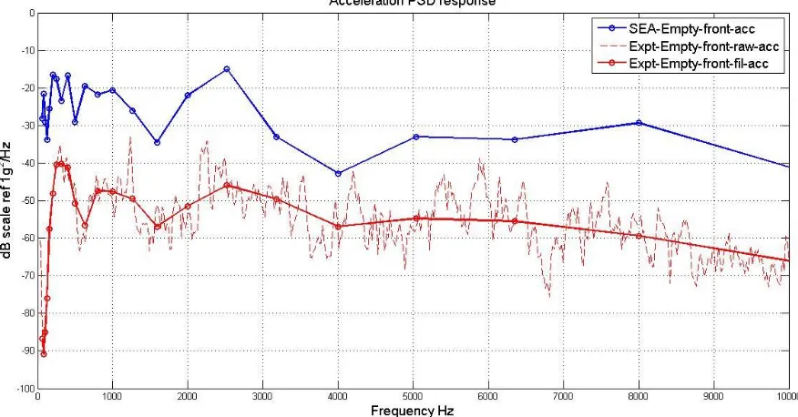
Figure 6.3:1: SEA vs Expt.: Empty Tank: Front: Acc. Response ... 62
Figure 6.3:2: SEA vs Expt.: 40% Filled Tank: Front ... 62
Figure 6.3:3: SEA vs Expt.: Empty Tank: Base ... 63
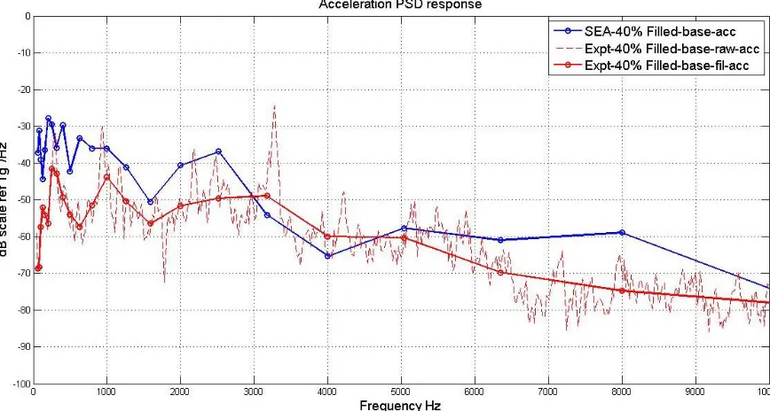
Figure 6.3:4: SEA vs Expt.: 40% Filled Tank: Base... 63
Figure 6.3:5: SEA: Empty vs 40% Filled Tank: Front ... 64
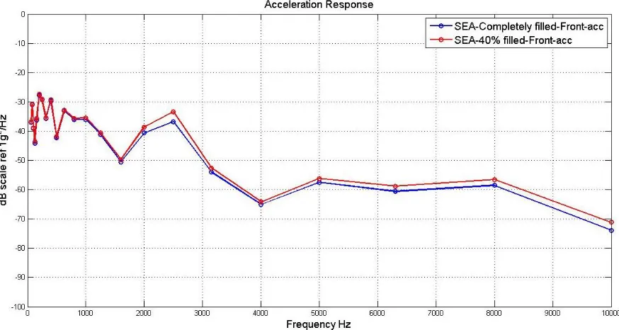
Figure 6.3:6: SEA: Completely Filled Tank vs 40% Filled Tank: Front ... 64
Figure 6.5:1: SEA vs Expt.: Far Field: Empty tank: Back face SPL ... 67
Figure 6.5:2: SEA vs Expt.: Far Field: 40% Filled Tank: Back face SPL... 67
Figure 6.5:3: SEA vs Expt.: Empty Tank: Near Field: Back face SPL ... 68
Figure 6.5:4: SEA: Empty tank: Far Field vs Near Field: Back face... 68
Figure 6.7:1: Variance study: Empty Tank: Base ... 71
Figure 6.7:2: Variance study: Filled Tank: Base ... 72
Figure A1:1: Two Plate System ... 80
Figure A1:2: Modal density Comparison: VA One & Theoretical Results ... 81
Figure A1:3: Coupling Loss Factor Comparison: VA One vs Theoretical Results ... 82
Figure A1:4: RMS Velocity Comparison: VA One vs Theoretical Results ... 82
Figure B1:3: Support mount: Expt. setup... 86
Figure B1:4: Elastic cord support: Expt. Setup ... 86
Figure B1:5: Base support bracket: Expt. Setup ... 87
Figure B1:6: Stinger & Connector: Expt. Setup ... 87
Figure B2:1: Accelerometer Specification ... 88
Figure B2:2: Microphone & Preamplifier specifications ... 89
Figure B2:3: Electromagnetic shaker specifications ... 89
Figure B3:1: 4 channel DAQ VI: Block Diagram ... 90
Figure B3:2: 4 channel DAQ: Front Panel ... 91
Figure B4:1: white noise VI: Block Diagram ... 92
Figure B4:2: white noise VI: Front Panel ... 93
Figure C1:1: Damping Calculation: Curve Fit ... 97
CHAPTER 1 1.1.Introduction
The interaction of solids with the interior or exterior fluid media plays a significant role in many engineering applications from civil [3] to aerospace [4] to automobile engineering [5]. For many such fluid structure coupling applications the closed form or analytical solutions are highly complex and difficult to obtain which led to greater emphasis on experimental testing and development of numerical techniques. The realistic limitations of testing and advancement of computational capabilities have contributed to considerable development of these simulation techniques.
The type of coupling between the solid and the fluid media determines the applicability of the numerical technique to simulate that coupling[6], [7]. If the fluid motion causes a significant deformation of the solid body leading to a change of boundary conditions for the fluid, then this coupling is called as a strong coupling or a 2 way coupling. A monolithic formulation in which a single system equation is solved can be applied for such type of coupling. If only the solid body vibrations cause a change in the fluid behavior then it is called as a weak coupling or a 1 way coupling for which a partitioned approach in which the structural and fluid system equations are solved separately can be applied.
For fluids enclosed within a container, the strength of coupling depends on the frequency range of interest along with fluid characteristics. The strong coupling between fluid and structure at low frequencies causes the phenomenon of ‘sloshing’ which can induce considerable dynamic stresses on the structure and can lead to component failures. Considerable research has been carried out to develop analytical and numerical techniques to model sloshing and has been experimentally verified to some extent as well [2], [8], [9].
At high frequencies this coupling is weak in nature, and affects only the surface vibrations of the structure. As a result, a partitioned approach can be used to compute the surface vibration response. The numerical techniques discussed above are deterministic in nature (i.e. for a given system, there will always be only one solution available). Thus, to account for geometric irregularities, a design of experiment approach is required to obtain an envelope of possible responses. This approach becomes cumbersome for high frequency applications as the computation time is dependent on the mesh quality. The modal assurance criteria (MAC) reduces with the increase in frequency and the contribution of the off diagonal terms increase significantly[10]. A study for experimental correlation and optimization by Marburg et al[11] showed that FEA process could be reliably used only up to a certain frequency limit.
1.2.Motivation
This phenomenon of fluid structure coupling was encountered during my stint as a computer aided engineering (CAE) analyst, in the Noise, Vibration and Harshness (NVH) group of the Research & Development (R&D) Dept. of Bajaj Auto Ltd. an automotive company in India. One of the persistent field complaints was regarding the jarring/rattling noise heard from the motorcycle during high speed use. Some standard tests were carried out such as the Pass-By-Noise (PBN) and Pass-By-Noise Source Identification (NSI) and the tank region was highlighted as the problem region. The gas tank of the motorcycle is a thin sheet metal structure with thickness approximately in the range of 0.8mm-1mm as shown in Figure 1.2:1. This tank was manufactured by the stamping process which led to thinning of the material near the curvatures. Seam welding along the flange and manual spot welding for mounting the required accessories resulted in a component with varying thickness and geometric irregularities. The gas tank weighed around 2-3 kg and has a capacity to contain 10-14 L of gasoline or approximately 8.5-12 kg of fuel with specific gravity of 0.8, depending on the make and model of the motorcycle. Static load tests revealed the ability of the gas tank to carry the weight of the fluid. However, impact tests and frequency response measurements with varying levels of liquid showed the variation of the tank surface response due to the fluid present in the tank.
The FEA simulation which was carried out using the partitioned approach is shown in Figure 1.2:2. For this simulation, the fluid chosen was water as its specific density is close to the
Figure 1.2:1: FSI simulation: Tank Model
Figure 1.2:2: Fluid Mesh Model
CHAPTER 2 2.1.Background
The development of Statistical Energy Analysis is credited to independent research on resonator vibrations carried out by R.H Lyon and P. W. Smith in the early 1960’s[12]. This method developed from the need of an approach which used as little system information as possible to predict a response which would be consistent with the results with some degree of variation, especially for problems which deterministic approaches couldn’t handle efficiently and effectively at that time. Statistical Energy Analysis is a method to calculate the flow and storage of dynamical energy in subsystems of a complex structure. Energy is provided to the system by external sources like acoustic pressure or mechanical excitation which is then dissipated in the components and transferred between different storage subsystems. As relative phase and amplitude of frequency response at individual points is unpredictable in nature, it was considered as a random variable, and hence the statistical response variables as the ensemble mean square value over space and frequency were considered[13]. Thus, the statistical nature of the input and response variables meant an undetailed model could be used for this analysis. There are different methods to formulate the energy transfer equations of Statistical Energy Analysis[12], [13] which have been briefly described below:
1. Mode Based Approach:
𝑃12 = 𝑔 ∗ [𝐸1− 𝐸2] ( 1 )
This method requires the strength of coupling to be weak, so that there is negligible intra subsystem interaction due to the other subsystem and hence is suited for vibro-acoustic problems which involve acoustic interactions between structures and enclosed fluid volumes.
2. Wave Based Approach:
In this method, the subsystems are expressed in terms of the superposition of travelling waves, and the interaction between the subsystems is evaluated from the wave transmission and reflection considerations at the junctions. Thus, the power transferred is a function of the wave impedances of the uncoupled systems at the junction.
This approach is used when there is a greater modal overlap causing many waves to contribute to the response at a frequency. As the waves are independent of the boundary conditions and depend only on the wave carrying medium, this method is used in case of strong coupling as those between structures especially if they are not isotropic.
While the approaches are different, the concept of mode-wave duality ensures the equivalency of the methods and hence at least theoretically it is possible to arrive at the same results using either of the methods mentioned above. The SEA module of ESI VA-One software suite makes use of the wave approach to calculate SEA parameters.
resulted in the development of experimental SEA[14], hybrid SEA (a combination of FEA and SEA)[15] and many parameter testing methods[16]–[19].
2.2.Parameter Definition
The basic principles of Statistical Energy Analysis are explained briefly in this section and the general form of the system equation is derived.
Subsystem
Mode Count
The mode count represents the number of resonant modes available to exchange energy between interacting subsystems and is dependent on the geometric and material properties of the system. It can be expressed as
Number of modes in a frequency range (ΔN) Modal density 𝑛(𝜔) = 𝑑𝑁
𝑑𝜔 𝑟𝑎𝑑/𝑠 or
Average frequency spacing between modes 𝛿𝑓 ={2∗𝑝𝑖∗𝑛(𝜔)}1 Subsystem Energy 𝐸𝑖
The total energy associated with all the modes in the given bandwidth of a subsystem is called as the energy of that subsystem. Hence, for a subsystem mass 𝑚𝑖 and mean square surface velocity, 〈𝑣𝑖2〉 the total subsystem energy is related to the spatially averaged surfaces responses as shown in equation ( 2 )
𝐸𝑖 = 𝑚𝑖〈𝑣𝑖2〉 ( 2 )
The assumption of equal distribution of energy among all the modes of the subsystem means that the total energy of the subsystem is the product of number of modes of the subsystem and the energy associated with each mode.
𝐸𝑖 = 𝑁𝑖 ∗ 𝜖 ( 3 )
Damping Loss Factor (𝜂𝑖𝑖)
The power dissipated in the subsystem is proportional to the average energy lost to the mechanical vibrations in the subsystem and is only dependent on the modal energy of that subsystem.
For an ith subsystem with damping loss factor (𝜂𝑖𝑖) the total modal energy (𝐸𝑖) the power dissipated is given as follows.
𝜋𝑖,𝑑𝑖𝑠𝑠 = 2𝜋𝑓𝜂𝑖𝑖𝐸𝑖 ( 4 )
Coupling Loss Factor (𝜂𝑖𝑗)
The coupling loss factor is associated with the average power flow between the coupled subsystems and thus is proportional to the difference in the modal energies of the subsystems. The CLF is dependent on the two coupled media as well as the geometric description of coupling (i.e. point, line or area coupled).
The power transferred between the ith and jth subsystem with coupling loss factors 𝜂𝑖𝑗and 𝜂𝑗𝑖 is given as
𝜋𝑖𝑗 = 2𝜋𝑓(𝜂𝑖𝑗𝐸𝑖 − 𝜂𝑗𝑖𝐸𝑗) ( 5 )
As the total energy of a subsystem is just the mode count times the modal energy, the coupling loss factor is subject to the reciprocity relation.
𝜂𝑖𝑗∗ 𝑁𝑖 = 𝜂𝑗𝑖 ∗ 𝑁𝑗 ( 6 )
External Excitation (Π𝑖)
2.3.Formulation
As statistical energy analysis is based on the theory of power flow and energy transfer, a common representation of SEA model can be shown as in the following figure.
Figure 2.3:1: Three Subsystem SEA model
The input power is an external user defined excitation for each subsystem of the model and thus for a ‘N’ subsystem model, it is a N x 1 column matrix
𝜋𝑖𝑛 = [𝜋1 𝜋2… 𝜋𝑁]𝑇 ( 7 )
𝜋𝑖 = 2𝜋𝑓𝜂𝑖𝑖𝐸𝑖 + 2𝜋𝑓 ∑ 𝜂𝑖𝑗𝐸𝑖 − 𝜂𝑗𝑖𝐸𝑗
𝑁
𝑗=1 𝑗≠𝑖
( 8 )
For the N=3 subsystem model shown, the above system of equations can be expressed in the matrix form as shown in equation ( 9 )
{ 𝜋1
𝜋2
𝜋3} = 2𝜋𝑓 [
𝜂11+ 𝜂12+ 𝜂13 −𝜂21 −𝜂31
−𝜂12 𝜂21+ 𝜂22+ 𝜂23 −𝜂32
−𝜂13 −𝜂23 𝜂31 + 𝜂32+ 𝜂33] {
𝐸1 𝐸2
𝐸3} ( 9 )
Or in simplified form
{𝜋𝑖𝑛} = 2𝜋𝑓[𝑇]{𝐸} ( 10 )
[𝑇] is called as the loss factor matrix as it is composed of the damping and coupling loss factors. This formulation is known as the unsymmetrical form of equations as T is not symmetrical. The T matrix can be made symmetrical using the reciprocity relation and the symmetric form, which is used for experimental SEA as well as for VA One SEA formulation. The symmetric system of equations is given as shown in equation ( 11 )
{ 𝜋1 𝜋2
𝜋3} = 2𝜋𝑓 [
(𝜂11+ 𝜂12+ 𝜂13)𝑁1 −𝜂21𝑁1 −𝜂31𝑁1
−𝜂12𝑁2 (𝜂21+ 𝜂22+ 𝜂23)𝑁2 −𝜂32𝑁2
−𝜂13𝑁3 −𝜂23𝑁3 (𝜂31+ 𝜂32+ 𝜂33)𝑁3
] { 𝐸1 𝑁1 𝐸2 𝑁2 𝐸3 𝑁3}
( 11 )
With
𝜂12𝑁1 = 𝜂21𝑁2 & 𝜂13𝑁1 = 𝜂31𝑁3 & 𝜂23𝑁2 = 𝜂32𝑁3 ( 12 )
2.4.Summary
To summarize, in this chapter, the formulation of Statistical Energy Analysis system of equation is studied and the significant model parameters are described. SEA uses a statistical approach to dynamical system and hence this method requires only a coarse description of the system to provide an initial idea about the trend of the system response.
As it is a power flow method, it provides the designer an idea about power transmission through the system and thus the contribution of different components to the system response can be identified.
CHAPTER 3 3.1.Thesis Scope
The scope and extent of this thesis project is defined in this chapter after reviewing the basic concepts earlier. As stated, the study of noise and vibration characteristics of the motorcycle gas tank was the motivation for this project. While the shape and capacity of the tank depends on the automobile type, it is usual for motorcycles to have a fuel capacity of 4-5 US gallons with an additional reserve of 0.6-1 gallon. The specific gravity of gasoline is in the range of 0.71-0.77 which means approximately 14-15kg of fuel mass. The shape of the tank is highly dependent on the packaging constraints and aesthetic requirements as shown in Figure 3.1:1.
Figure 3.1:1: Gas Tank (JP cycles)
3.2.Design Parameters
In this project, the tank dimensions were dependent on the design requirements, manufacturing process and the experimental testing limitations.
Design Requirements
While the tank used in real applications has curvatures and complicated shapes, the design was simplified to produce a simple parallelepiped tank model. It was decided to make one dimension of the tank significantly larger than other similar to the actual gas tank. Water was used as fluid instead of gasoline to avoid any potential conflagration issues. The acoustic pressure modes for water were dependent on the tank dimensions. After some initial calculations of fluid volume, the tank dimensions were chosen to be 18 in X8 in X8 in with a thickness of 0.036 in.
Manufacturing Constraints
The simple tank design and decision to manufacture the tank using standard welding technique of gas welding reduced the manufacturing time. However, it was found that there was too much distortion during the welding process for sheet metal with thickness 0.036 in. In order to this thickness of sheet metal, it would have been necessary to use dedicated fixtures for supporting tank surfaces during welding.
Experimental Testing Constraints
As the thickness of the tank increases, the excitation frequency required for fluid structure interaction increases. The accelerometers used have an operable frequency range of 5-10000 Hz which though lowest among all the testing equipment used was still sufficient for testing purposes. As Statistical Energy Analysis assumes that resonant frequencies and modal behavior is unknown, simply increasing the frequency range of testing could lead to measuring the fluid structure interaction effects on the tank surfaces. To avoid the necessity to use some lifting mechanism for tank testing, the dimensions of the tank were not altered significantly. Instead, it was decided to increase the frequency of excitation up to 10,000 Hz which is the limit of the test setup.
Figure 3.2:1: CAD Tank Model
3.3.Preliminary Testing
Figure 3.3:1: Preliminary Test Setup
Reciprocity theorem
Figure 3.3:2: Reciprocity Top Side
Symmetry
Figure 3.3:3: Symmetry: Front Face: Longitudinal Direction
In Plane Vibrations:
This measurement was carried out to check the contribution of different modal subsystems to the vibration response of the plate. Theoretically, it is proven that the flexural modes dominate the surface responses. A tri axial accelerometer was used and each face was excited in the three orthogonal directions. The accelerometer was mounted in such a way that the Z direction was always perpendicular to the plane of the face. For excitation along the in plane directions, the impact was made at the boundary normal to that direction. As can be seen from Figure 3.3:5 and Figure 3.3:6, the flexural response does dominate the vibration response of the plate even if the excitation is provided to the in plane vibration modes. This is useful, as further measurements can be made with a uniaxial accelerometer which can measure only out of plane responses.
Figure 3.3:6: Y excitation: Top Face
3.4.Summary
In this chapter the scope of this thesis project was discussed. It was decided to experimentally determine the surface vibration and acoustic responses of the tank and use the FEA and SEA software modules of the ESI Vibro-Acoustics software suite to simulate the experiment. The design and manufacturing considerations for determination of the tank dimensions were explained. To mimic the application, it was decided to excite the tank only from its mounting points. It was decided to measure responses over a frequency range from 0 Hz – 11220 Hz using one-third octave frequency bands to see the effects of fluid structure interactions. The testing procedures and results are explained in detail in the next chapter.
CHAPTER 4 4.1.Experimental Setup
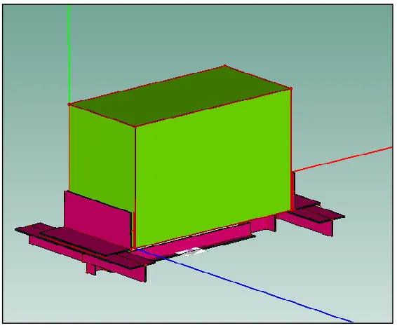
The experimental setup and testing procedures are explained and the results are discussed in this chapter. It was decided to replicate the boundary conditions and the excitation experienced during the real life use of the gas tank. To achieve this, a base structure was designed from Aluminum T shaped and L shaped channels and the tank was mounted on this structure as shown in Figure 4.1:1. The details of this model are attached in Appendix B. This arrangement allowed for simulation of the tank excitation via its connections to the vehicle frame.
Figure 4.1:1: CAD Model: Tank Structure
Figure 4.1:2: Experimental Setup
4.2.Experimental Apparatus
In this thesis, vibration and acoustic measurements were carried out to measure the tank responses for varying liquid levels. The following transducers were used for experimentation. Accelerometers
PCB ICP uniaxial shear accelerometers of the model type 352C33 are used for measuring the flexural vibrations of the tank surfaces. With a sensitivity of 100mV/g and a frequency range of 0.5Hz to 10,000Hz, these accelerometers were suitable for the testing purposes.
Microphones & Pre-amplifiers
Electromagnetic Shaker & Amplifier
B&K LDS V203 low force range shaker with a frequency range of 5-13,000Hz was used along with PA 25E power amplifier to excite the test setup.
A slender cylindrical steel rod of 12 in was manufactured to connect the shaker to the test component. The purpose of this rod called ‘stinger’ is to transmit only the axial force from the shaker to the tank and to decouple the shaker mass from the lateral and transverse fluctuations of the tank.
Force Transducer
PCB ICP force transducer of model type 221A05 with a sensitivity of 2.25 mV/N was used to measure the force. The force transducer is connected between the stinger and tank and is used to measure the net dynamic force on the tank.
The complete specifications of these instruments are attached in Appendix B. 4.3.Signal Generation
There are various deterministic or random signals[20] which can be used to excite the test structure for the measurement of the vibration responses. Deterministic signals like swept sine, saw tooth waveform or sine chirp can be described by mathematical functions. Sinusoidal or sine sweep excitation can provide a very good response spectrum and is used for modal analysis. However, it is the slowest technique for signal excitation, as each spectral frequency is excited individually and there is some delay time for system stability.
density varies inversely with frequency. Random signals excite the structure with varying amplitudes and frequencies and tends to average out the responses over time. While there are some leakages due to side lobes of window functions, this type of input signal characterizes most of the real life excitations and hence, a uniform white random noise was selected for system excitation.
National Instruments (NI) LabVIEW was used to generate the uniform white random noise in different frequency bandwidth. The Figure 4.3:1 shows the power spectral density (PSD) (ref 1V2/Hz) of a uniform white random signal within a frequency range of 0-11360 Hz with a maximum amplitude of 0.5V rms.
Figure 4.3:1: Input Signal PSD
accounting for the difference in sampling frequencies of these two systems is explained in Appendix B.
It was decided to excite the tank over a large frequency range as the modal information of the system was unknown. Hence, input signals up to 11,360 Hz were generated in different frequency bandwidths which just reached the limit of the functional range of the accelerometers.
4.4.Data Acquisition Parameters
General purpose coaxial cables were used to connect the transducers to BNC cables. No separate signal conditioning unit was required as the transducers used were integrated piezoelectric transducers. National Instruments PXI chassis 1031 with a 4 channel 24 bit analog input data acquisition card PXI 4462 was used for acquiring and processing the response signals. The inbuilt analog to digital convertor of NI was used for processing the data. NI LabVIEW, a system design platform and development environment using graphical language was used for specifying the important data acquisition parameters and carrying out data manipulation and post processing.
experimental studies [14] mention measuring responses at 3-5 locations for good spatial averaging. In order to account for the geometric irregularities, it was decided to measure the 15 responses each on 16 in X 10 in side and 16 in X 8 in side. The measured acceleration response was spatially averaged and its power spectral density with ref to 1𝑔2
𝐻𝑧 was calculated. In order to study the influence of fluid on the overall tank response, it was decided to measure the sound pressure level around the tank in the anechoic chamber. For the acoustic response measurement, the microphones were mounted along the normal direction to the tank surface. Near field acoustic response (~ 2 in away) and Far field acoustic response (~ 40 in away) was measured for the four vertical sides for both the experimental conditions. The near field experiment setup is shown in Figure 4.4:1.
Figure 4.4:1: Near Field Experimental Setup
4.5.Experiment Description
In this section the results of the experiments are explained and some observations are made regarding the behavior of the fluid tank system. The tank surfaces are named as shown in Figure 4.5:1. The L shaped mounts are welded to the left and the right face of the tank. These mounts
are used for suspending the tank in the anechoic chamber.
Figure 4.5:1: Tank Nomenclature
The vibration and acoustic measurements are performed on both the empty and fluid filled tank. While many experiments were carried out, some of the representative tests are discussed and the results plotted in this chapter.
Table 4.5-1: Experiment Description Experiment Type Tank Setup Description Transducer mounting Measurement Location Measurement Parameter Vibration
Empty Tank On Tank
Front Face Base Face Right Face
Acceleration Force 40% Filled Tank On Tank
Front Face Base Face Right Face
Acceleration Force 70% Filled Tank On Tank
Front Face Base Face Right Face Acceleration Force Acoustic
Empty Tank Near Field (~ 2’’) Front Face Back Face Right Face Left Face Sound Pressure Level
40% Filled Tank Far Field (~40’’)
Front Face Back Face Right Face Left Face Sound Pressure Level
Based on the sampling rate and the number of samples, the frequency step size in the power spectral density plot is almost 20Hz. This data was averaged over the one-third octave frequency bandwidths and the raw PSD data along with the bandwidth averaged PSD data is plotted in this section. This is done as the bandwidth average data would be enable a better understanding of the vibration trends of the tank. The raw PSD data is plotted with dotted line and its one-third frequency bandwidth averaged response curve is plotted as a bold dashed line in the following plots for comparison.
tank experiment to verify the similarity of the input for both testing conditions as shown for the base in Figure 4.5:2 and the front face in Figure 4.5:3.
The power spectral density of the acceleration response for the tank faces for the different setup conditions is compared to show the influence of the fluid on the vibration response of the surface. The response for base (Figure 4.5:4), front (Figure 4.5:5) and the right face (Figure 4.5:6) are attached. The response for the front face for different fluid levels is also studied as
shown in Figure 4.5:7.
Experimental Results: Vibration Testing
Net Dynamic Force Response
Acceleration Response
Acceleration Response
4.7.Observations – Vibration Response
The comparison of net dynamic input forces for the empty tank and 40% fluid filled tank in Figure 4.5:2and Figure 4.5:3 show a good similarity. The fluctuations can be attributed to the additional inertial mass of fluid and the change of the elastic cord stiffness. This fluctuation isn’t large enough to cause non-linear or indirect coupling and hence the two experimental conditions shouldn’t violate the basic assumption of small displacements.
The general effect of addition of fluid has been to reduce the amplitude of the vibration response especially in the high frequency region. This is seen explicitly in the response of the front face (Figure 4.5:5), while the base face response (Figure 4.5:4) shows some interactions at lower frequencies as well. It is expected that the base response would be affected the most by the addition of fluid, due to the inertial effects and the damping of the fluid.
The acceleration response of the right side doesn’t indicate such a significant fluctuation in Figure 4.5:6. This could be due to the additional stiffness of the face by welding of the thicker mount. This could reduce the influence of the fluid on the vibration response of the face as the face isn’t a thin enough sheet metal surface. The front face response due to varying fluid volume in the tank shown in Figure 4.5:7
4.8.Experimental Results: Acoustic Measurements
Sound Pressure Level Response
Sound Pressure Level Response
4.9.Observations – Acoustic Response
The far field acoustic response for the front and back faces of the tank is similar as shown in Figure 4.8:1. This similarity is expected due to similar dimensions and properties of the faces. The small variations can be attributed to the geometric irregularities and the effect of the surrounding structures on the measured response. Due to this type of behavior, only the responses of the back surfaces were shown in this chapter. The observations about the experimental trends should be valid for other faces. The far field acoustic response for the back face for empty and 40% fluid filled tank (Figure 4.8:2) shows the reduction in acoustic sound pressure level at high frequencies due to the presence of fluids. This is consistent with the acceleration response of the faces which reduce due to addition of fluid volume. The variation of acoustic response in the low range up to 3000 Hz was unexpected and may be due to acoustic inputs from the base structures and the surrounding bodies in the anechoic chamber.
The near field and far field comparison of the acoustic response (Figure 4.8:3) indicates that the near field sound pressure is higher than the far field response. This is expected, as the sound pressure decreases with the increase in distance from the sound source.
4.10. Conclusions
the empty tank is to reduce the amplitude of the response. Increase in the fluid volume from 40% to 70% of the tank volume did not have a significant effect on the vibration response. The experimental results show influence of some external parameters as seen from the fluctuations in the input force responses and acoustic responses. The acoustic responses measure the contribution of all the participating components and hence is more sensitive to the experimental setup conditions.
CHAPTER 5 5.1.Introduction
It was found that the commercial use of Statistical Energy Analysis as a simulation tool was not as wide spread as other Finite Element Analysis formulation codes. While there were some basic standalone software codes for SEA modeling and simulation, only a couple of well-established software modules were found. The Vibro-Acoustics software suite of ESI group contained both the SEA and FEA modules for simulation purposes. The advantage of using the same software suite for both simulation methods is in the compatibility of the modeling and system parameters. It was easy to define the entire model for SEA simulation and simply convert it into a FEA model without redefining a lot of the system parameters. The same NASTRAN solver was used and hence the solver parameters and solver efficiency were the same for both the modules.
In this chapter, modelling and simulation of the test setup is described with an explanation of the underlying assumptions and the results are compared for the simulation methods. The appropriate use of the SEA module for a simple two plate system is verified by comparison with theoretical results in Appendix A.
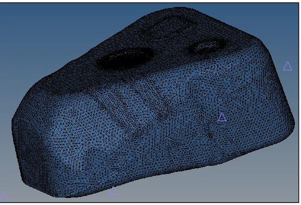
5.2.SEA Simulation model
Figure 5.2:1: SEA Model Setup
The tank faces are assigned a steel material with thickness 0.06 in and the L mounts are assigned the same steel material and have a thickness 0.12 in. The seam welding along the face edges is defined by a line junction between the faces. Line mass is added to the junction to account for additional filler material mass. The welding connection between the L mount and tank surface is along the vertical edge as shown and not across the upper edge of the plate. In order to model welding along the same edges as the manufactured tank, the coincident node technique was used. Hence, two separate nodes were created close to each other and were defined in the face subsystem and the mount subsystem. Thus, it was possible to define the line connection along this edge, without specifying any other contact region.
To measure the sound pressure level at a fixed distance from the model, a semi-infinite fluid region was created at distances specified from the experimental testing. This acted like an energy sink, and stored the energy transmitted from tank without reflecting it back or interacting with the system.
A NASTRAN internal solver is used for calculation and the frequency was chosen from100 Hz to 16000 Hz in one-third octave frequency bandwidths and acceleration responses were computed along with other parameters for comparison.
5.3.FEA Simulation Model
Figure 5.3:1: FEA Model Setup
The response was measured in the normal direction to the tank faces and in order to compare the FEA responses with the spatially averaged SEA responses, approximately 30 locations were used for response measurement in the simulation and the averaged response was used.
5.4.Assumptions
As explained in the previous chapter, the free-free boundary condition is used to isolate the tank from the surroundings. This boundary condition can be simulated by not applying any constraints to the model.
high frequencies this assumption may not hold and hence, as will be explained in the next chapter, a more detailed model of the test setup was created for correlation purposes.
As SEA responses are not affected significantly by minor geometric irregularities of holes and plate warping, it was decided to model the tank faces as simple rectangular plates. As the L mounts are bolted to the T beams, the influence of mounting holes on vibration response is reduced, and hence L mounts are also modeled without the mounting holes.
While the damping loss factor for the tank surfaces was calculated, the damping loss factor for water was assumed to be 20%. [21] The damping loss factor of air is taken as 1%.
The theoretically calculated modal density and coupling loss factors were used for simulation as these are not user dependent but geometry and material dependent. For a simple plate, the out of plane flexural vibrations were observed to be more
5.5.Results
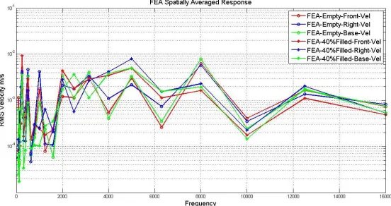
With these assumptions in place, it was decided to compare the responses of the SEA and FEA simulation models for a unit force excitation and a constant damping loss factor of 0.1% as these parameters are unknown and assumed constant during the initial design process. Usually in such cases, simulation tools are used to compute the response trend lines and study the behavior of the system. For this reason, the results of both the models for an empty tank and a completely filled fluid tank were compared for initial estimation of computational time and accuracy. The flexural or out of plane RMS velocity responses of three sides of the tank are plotted for the above mentioned input conditions. A large frequency range was chosen for this study and the responses are calculated in one-third octave frequency bandwidths.
RMS Velocity Response: SEA: Completely Filled vs Empty Tank
5.6.Observations
It can be seen from Figure 5.5:1 and Figure 5.5:2 that at low frequencies the SEA velocity RMS response is significantly larger than the FEA velocity response. As the frequency increases, the FEA and SEA responses start to converge. One of the possible reasons for this could be the increase of the number of modes participating in the energy transfer with frequency. At low modal densities the SEA assumption of equal distribution of energies for all the subsystem modes might be violated and hence, the response might be a bit on the higher side.
The FEA response comparison for a completely filled tank vs an empty tank exhibits more fluctuations over the frequency range than the SEA response comparison for the same case as seen in Figure 5.5:3 and Figure 5.5:4. This is to be expected as SEA is an averaged response over the entire surface and while the FEA response is measured at 20 locations, it is still not ideally spatially averaged.
It can be seen that the fluid filled tank response is higher than the empty tank response in some frequency bandwidths for FEA simulation method (Figure 5.5:3) while the response decreases almost uniformly for all the surfaces for the SEA method. (Figure 5.5:4). One of the reasons for this could be the difference in the method used for the
computation of the fluid structure coupling for these simulation tools
filled tank, it took approximately 3.5 hrs. for the software to complete all calculations for FEA simulation. In comparison, SEA computation took only a couple of minutes to complete its calculations. All the simulations were carried out on the same DELL Precision T5610 workstation with no programs running in the background.
The power flow plots for SEA method provided insights into the contributions of different components to the overall response of a surface similar to the transfer path analysis approach for FEA studies. However, this being an inherent part of computation required no extra setup which was an added advantage.
Thus, SEA is a valid alternative to FEA for simulation purposes, especially in the high modal density applications. With this validity established, it was decided to check the correlation of SEA results with experimental data in the next chapter.
5.7.Experimental SEA
As explained before, out of the four critical parameters of SEA methodology, the specification of the damping loss factor of the components and power input to the system are user dependent, while computation of modal densities and coupling loss factors are geometry and material dependent.
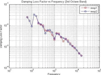
Damping Loss Factor
There are several methods to measure the damping factor of lightly damped materials such as the half power method and decay method[12], [14], [16]. In this project, the decay rate method was used for experimental measurement of the damping loss factor.
𝐶~𝐴𝑒−𝜔𝜂𝑡 ( 13 )
Thus, once the peaks in the response are identified, a curve fitting method can be used to fit an exponential curve with the constant 𝐴 and the damping loss factor 𝜂 as the variables.
A transient excitation was applied with a modal impact hammer and the acceleration frequency response was measured on the tank face at 2 response points. The damping loss factor was computed over the entire frequency range as well as for one third octave bandwidth limited frequency range.
The average damping loss factor over the entire frequency range is 𝜂𝑖𝑖~ 0.14% which is consistent with the defined values of damping for steel. The damping loss factor was measured for two faces and as it is a function of the material type the same damping loss factor was used as an input for the tank faces for both the simulation techniques.
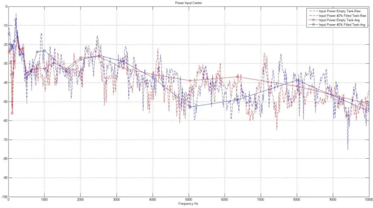
Input Power
Input power is usually computed with an impedance head using the mobility and point force data to compute the power. However it is possible to derive the input power using accelerometer and force transducer data[22], mounted at different locations if the data acquisition starts simultaneously for good phase matching. The input power can be computed as the cross correlation at 𝜏 = 0 of the force and accelerometer signals by the formula below.
𝑅(𝑓, 𝑣, 0) = − ∫ 𝐼𝑚𝑎𝑔 {−∞∞ 𝐺(𝑓,𝑎,𝜔)𝜔 } 𝑑𝜔[22] ( 14 )
Where 𝐺(𝑓, 𝑎, 𝜔) is the cross spectral density of force and acceleration.
Figure 5.7:2: Input Power
The modal density of a plate is a property of the geometrical dimensions and material properties. Considerable work has already been carried out to experimentally verify the modal density [18], [23] by measuring the frequency response function for the plates.
CHAPTER 6 6.1.Introduction
A significant difference in the amplitudes of the SEA response and the experimental results can be seen. A similarity in the trend of the vibration response between the two methods is seen as well. This difference is observed in the vibration responses for the other tank faces as well. Thus, it can be said that this response behavior is characteristic of the SEA simulation model and hence factors which could affect the entire tank responses were considered for refinement of the SEA model. As a result, minor details like holes on the top and bottom face for water inlets and outlets, or on the L mounts for bolts are not considered significant. This difference could be attributed to several structural factors which could affect the results in varying degrees. The coupling loss factors used are theoretically derived and there may be some variation in the behavior of the experimental coupling loss factors especially with varying modal densities. However, this has been verified to some extent [16], [17] and as explained before, as this should be a geometrical factor, it was decided to use the theoretical values. The use of elastic cords to simulate free-free conditions is an approximation which isn’t considered during the SEA simulation. This assumption is shown to affect the lower frequencies much more[24] and hence isn’t considered for the model refinement.
Figure 6.1:2: SEA: Refined model
Some simplifying assumptions were made when this refinement was carried out to reduce the SEA modelling time. The L mounts of the tank were bolted to the support structure. As the L mounts were bolted at 3 locations over the surface, this bolting connected was modelled as a line junction in SEA simulation. Similarly, the bolting connections between the different brackets were also modelled as line junctions, with the lines extending for approximately the projected bolt head length. The brackets connecting the tank structure to the elastic cords were not modelled as these don’t affect the tank vibration response directly.
As the tank support structure is now modelled, the input power was calculated and applied at the excitation point, which is approximately the center of the structure as seen in the Figure 6.1:2. It was expected that as the accelerometer is mounted almost exactly on top of the force
The vibration and acoustic responses for the SEA simulation model were computed again after these refinements and are used for comparison with the experimental results as shown in the next section.
6.2.Comparison Summary
In this section, the SEA simulation and experimental testing results are compared for different tests as mentioned in Table 6.2-1.
Table 6.2-1: SEA vs Experimental Results: Comparison
Experiment Type Tank Setup Condition Results Plotted Measurement Location Measurement Parameter Vibration
Empty Tank SEA
Expt.
Front Face
Base Face Acceleration Filled Tank SEA
Expt.
Front Face
Base Face Acceleration Empty Tank
Filled Tank SEA Front Face Acceleration
40% Filled Tank SEA Front Face Acceleration
Acoustic
Empty Tank Far Field
(~ 40 in)
SEA
Expt. Back Face
Sound Pressure Level Filled Tank Far Field (~40 in) SEA Expt.
Back Face Sound Pressure Level Empty Tank
Near Field (~ 2 in)
SEA
Expt. Back Face
Sound Pressure Level Empty Tank
Near Field Far Field
SEA Back Face Sound Pressure
Vibration Response:
The spatially and frequency averaged acceleration response for the front face is shown in Figure 6.3:1 for the empty tank case to study the effect of model refinement on the simulation results
as compared with the experimental test results. The response for the filled tank is also compared with the test results for the front face in Figure 6.3:2. Similar comparison for the bottom surface of the tank is made in Figure 6.3:3 and Figure 6.3:4 to highlight the similarity of the response trends for SEA and experimental correlation. The SEA response for the empty tank and the fluid filled tank is plotted for the front face to show the influence of the fluid structure coupling on the SEA simulation results. The SEA simulation results for the front face with different fluid levels is shown in Figure 6.3:6.These results are compared with the similar plot for experimental testing and some conclusions are made regarding the validity of observations made from the simulation responses.
Acoustic Response:
6.3.Results - Vibration Measurements
SEA vs Experimental Results: Front Face
SEA vs Experimental Results: Base Face
Figure 6.3:3: SEA vs Expt.: Empty Tank: Base
SEA Results: Front Face
6.4.Observations – Vibration Measurements
It can be seen from Figure 6.3:1 that the SEA model refinement has increased the accuracy of the model to simulate the experimental results as compared to the results shown in Figure 6.1:1 As with any correlation case, some differences are expected between the test data and the simulation data which is visible in these plots.
The comparison of the acceleration response for the front face empty tank in Figure 6.3:1 indicates that the SEA response is higher than the experimental results in the low frequency region. This is expected as the modal density is low in this frequency region which would cause violation of the assumption of the equipartition of energy in every frequency bandwidth. This was observed in the previous chapter when the SEA and FEA responses were compared over similar frequency ranges. A better correlation is seen between 3000 Hz – 6000 Hz with some deviation after that frequency. As the high frequency vibrations are sensitive to the accelerometer mounting and setup conditions, there is some uncertainty associated with the measured test data as well.
The response comparison for the front face indicates greater correlation for the empty tank case than the 40% filled condition as seen from Figure 6.3:1 and Figure 6.3:2 which may be due to the influence of the fluid structure coupling effect. As the tank is partially filled during experimental testing, the coupling during experimental testing for the front face is complex and may not be captured accurately by the SEA simulation method.
behavior can be attributed to the simulation parameters rather than some local factors. In case of the base face, it can be seen that the acceleration response from SEA simulations for the empty tank case as well as the filled tank case correlates well with the test data. This is expected as the entire base face is the wetted area for the fluid structure coupling. Thus, the entire flexural subsystem of the base plate participates in the energy transfer with the fluid body and hence, this effect is simulated by SEA much more effectively.
The SEA simulation trend lines of the spatially averaged surface responses for the empty tank and filled tank condition in Figure 6.3:5 indicate negligible influence of the fluid on the response at low frequencies, but considerable damping at high frequencies. It indicates the increasing influence of the fluid coupling on the surface vibration response which is due to the increase in the participating fluid modes. Comparison with experimental testing for the same conditions show similar effect of the fluid coupling. However, the experimental testing results indicated a fluctuation in the vibration response in the low frequency range (below 2000 Hz) due the fluid structure coupling which is not seen in the SEA simulation.
The SEA acceleration response for the completely filled tank and a 40% filled tank for the front face is shown in Figure 6.3:6. It can be seen that there is very small difference in the vibration response which is similar to the experimental results for the acceleration response for varying fluid levels. This indicates that the front face isn’t affected as much by the inertia of the fluid volume as by the fluid damping.
6.5.Results – Acoustic Response
Figure 6.5:1: SEA vs Expt.: Far Field: Empty tank: Back face SPL
Sound Pressure Level Response
6.6.Observations - Acoustic Measurements
It can be observed that there is a greater deviation for the acoustic responses as compared to the vibration responses. The SEA acoustic response plotted in this Chapter is only due to the individual tank surface normal to that location. Thus, this deviation is expected as the SEA simulation tool can measure the sound pressure level by a single panel while the sound pressure level measured during the experimental testing will have contributions from all the setup components.
The Far field sound pressure level response for the back face is shown in Figure 6.5:1 for the empty tank condition. It can be seen that the acoustic response trend line is similar to the acceleration response trend line shown in Figure 6.3:1 for the front surface for the SEA simulation response. This indicates that the acoustic sound measured at some distance from the tank is dependent on the vibration of the tank surface. This is consistent with the line of thought that the variation in the vibration response due to the fluid structure coupling can cause a change in the measured acoustic sound.
The near field acoustic response for an empty tank is shown in Figure 6.5:4 indicates very little correlation with the test data. Near field response is greatly influenced by the edge effects and is very sensitive to the measurement parameters. In addition, the near field response isn’t particularly applicable to the problem inspiration as the noise was heard by the rider and in the Pass by Noise test, which measures the sound pressures at a distance from the vehicle. Hence, the representation of the near field noise is for the sake of completeness and this lack of correlation wasn’t investigated further.
The far field and near field SEA response for the empty tank back surface as shown in Figure 6.5:4 indicates the same trend as the experimental results for the same conditions. This is
expected as the response should reduce with an increase in the distance from the sound source. Thus, the vibration and acoustic responses for the SEA simulations and experimental testing were compared and a good correlation was found between these responses. In the next section, the variance studies are carried out to account for the response variations due to the coarse modelling of the experimental setup.
6.7.Variance Study
model doesn’t account for some of the details like bolting locations, holes and additional masses a lower confidence level can be used. It can be observed from the plots that the trend of the SEA response remains the same irrespective of the confidence level.
It can be seen that by accounting for the variance of the setup parameters, the SEA response can match the experimental testing response for a large frequency range of operation. The variance of the SEA response is greater in the lower frequency range to account for the low modal density and it tapers off as the frequency increases.
Figure 6.7:2: Variance study: Filled Tank: Base
Chapter 7 7.1.Project Summary
In this thesis project, the applicability of Statistical Energy Analysis (SEA) as a design tool for quick initial computations was studied by investigating the influence of fluid structure coupling on the vibration behavior of thin sheet metal structures. An experimental setup was manufactured and vibration and acoustic responses were measured in the anechoic chamber of NC State University as described in Chapter 4. The ESI VA One simulation modules of Finite Element Analysis (FEA) and Statistical Energy Analysis (SEA) were used to simulate the experimental setup and the results of SEA were compared with the FEA results for accuracy in Chapter 5. After some refinement of the SEA simulation model, the results of the experimental testing were compared with SEA responses in Chapter 6. Based on these comparisons, the following conclusions were reached in this thesis
7.2.Conclusions
The restrictions of using FEA techniques for high frequency simulation and the limitations of deterministic methods to handle the inherent variations of the manufacturing process were highlighted. The FEA techniques can be used for the low frequency vibrations but the modal correlation reduces at high frequencies.
The influence of modal density on the SEA responses was seen at low frequencies as the SEA responses were considerably higher than the FEA responses and the experimental responses as well.
Experimental testing of the fluid structure coupling was carried out in the anechoic chamber and the influence of this coupling on the vibration and acoustic response was studied.
It could be seen that there is a change in the vibration behavior of the tank surfaces due to the addition of the fluid volume. This vibration change affects the acoustic response of the tank and thus the noise signature of the vehicle could be modified.
The preliminary impact hammer tests indicated the irregularities in the experimental setup which proved the viability of SEA to model such real systems.
Some of the test parameters were used as inputs to the SEA simulation method for correlation purposes. It was seen that the vibration and acoustic response of SEA is greatly dependent on the measurement of input power.
Comparison of the experimental results with SEA simulation was done to refine SEA model and a good correlation was seen for the vibration and acoustic responses. It was seen that acoustic responses are more susceptible to external influences which affected the correlation.
Variance studies used to account for irregularities of surfaces and coarse modelling of the experimental setup indicated that the SEA response is within the range of the experimental results.
Thus, the feasibility of SEA as a simulation tool for design purposes, especially in the high frequency region was shown in this thesis project. In the next section, some of the possible research directions are discussed.
7.3.Future Work
For initial stages of design process, optimization of geometric parameters within the design constraints is of significance especially in the highly competitive automobile sector or aerospace applications. The shape and size of the sheet metal panels determine the vibration and acoustic response of the system and hence, these parameters can be optimized for the required response.
The critical parameters of Statistical Energy Analysis such as modal density and coupling loss factors are dependent on the geometric dimensions and material properties and hence these basic dimensions can be used as design variables for optimization. The Design of Experiments approach to study parameter sensitivity can provide results very quickly when used with SEA rather than FEA simulation.