Design and Development of a Portable E-Nose for Gas Identification

Design and Development of a Portable E-Nose

for Gas Identification

Namrata Kataki1, Riku Chutia 2

Assistant Professor, Dept. of ECE, GIMT, Guwahati, Assam, India

Assistant Professor, Dept. of ECE, Tezpur University, Assam, India

ABSTRACT: A portable electronic nose (E-nose) has been designed and equipped with analysis software for the automated detection of odour released from chemical sample. An array of six metal oxide sensors is used for detecting volatile organic compounds. This E-nose is microcontroller based and is embedded with ANN based pattern recognition algorithm. The system is trained to identify nine chemical odorant samples irrespective of their concentrations.

KEYWORDS: ANN- artificial neural network, E-Nose-Electronic nose, VOC- volatile organic compound, PPM-Parts Per million

I. INTRODUCTION

Electronic nose (E-Nose) or artificial nose is defined as an instrument that comprises an array of electronic chemical sensors with partial specificity and a pattern recognition system capable of recognizing simple or complex odour [1]. Electronic noses are being developed as systems for the automated detection of odours, vapours, and gases. An electronic nose must be capable of identifying low concentrations (PPB-PPM) of chemical signals in an odorous environment with detection times of less than one second [2].

II. RELATED WORKS

In [1] authors sighted a brief history of E-Nose and different “instruments” used to evaluate the smell or flavour of products such as perfumes (cosmetics, soaps, etc.), food stuffs (fish, meat, cheese etc.) and beverages (beer, whisky, c offee, etc.). In [3], authors described some conventional analytical methods such as gas chromatography and gas chromatography-mass spectrometry to measure the physicochemical properties of a product. However, they also mentioned that these methods are not only time-consuming but the results are often inadequate due to some unclear relationship between the physicochemical properties of the odorant molecules and their sensory impact. Application of ANN in E-Nose is explained in [4]. In [5] Pattern recognition is implemented in E-Nose. Preprocessing techniques and various parametric analysis techniques are discussed in [6].

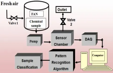
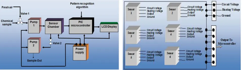
III. BLOCK DIAGRAM REPRESENTATION OF THE PORTABLE E-NOSE

The basic block diagram representation portable E- Nose includes three major parts: (a) Sample delivery system, (b) Detection system and (c) Computing system.

The sample delivery system enables the preparation of standard gas mixtures of VOC. The system then injects this standard sample into the detection part of the electronic nose. The sample delivery system is essential to guarantee constant operating conditions.

The detection system consists of an array of gas sensors. When in contact with volatile compounds, the sensors experience a change of electrical properties. Each sensor is sensitive to all volatile molecules but each sensor responses in their specific way. A specific response is recorded by the electronic interface transforming the signal into a digital value. Recorded data are then computed based on statistical models.

Fig 1: Block diagram of the designed portable E-Nose

IV.DESIGN OF THE SYSTEM

The design and development of a portable E-Nose can be divided in two parts – (a) Training of the system and (b) Sample identification. The training includes - data collection as well as classification of different odour samples using pattern recognition technique.

The data collection system is a handhold device mainly comprising of gas sample container with “standard” gas sample, a micro pump, a sensor chamber containing an array of sensors and data acquisition card. The collected data are used to train the system with pattern recognition algorithm (ANN) to classify different chemical samples.

Fig 2: Block diagram of sample collection and classification

The word “Standard” gas sample implies a gas mixture of volatile organic compound (VOC) accurately prepared by introducing known volumes of liquid sample into gas-filled container of fixed dimensions at atmospheric pressure [14]. The response of a gas sensor is not absolute; for the same gas sample different responses are observed at different concentrations. Therefore responses must be calibrated against accurately prepared mixtures of known composition. A low concentration (ppm level) standard gas mixture of VOC is prepared by using the following– [14]

=

, ..…….. (1)

= ………..(2)

Where C is concentration of the liquid , νgc is volume of the chamber, dliq is density of the liquid, Vliq is amount of

liquid to be injected, R is ideal gas constant, T is laboratory temperature, M is molecular mass and P is laboratory pressure.

The sensor chamber, where the six TGS sensors were assembled in an array and the inlet of the chamber was connected to the pump. Before sampling, the sensors were heated by a 5V power supply, while the pump was ON. When the sensors get sufficiently heated and the response of the sensors got to the baselines, the system was ready for sampling. Then the accurate gas mixture was injected to the gas container producing standard gas vapours of known concentration. The pump now, pushed the vapor of the sample around the inlet into the sensor chamber, and the sensors

Preparation of standard gas

sample

Detection system (Array of gas sensors)

Data Preprocessing Pattern

Recognition system Classification /

in the chamber immediately responded to the vapour. When the response time of the sensors was enough for extracting robust signals the lid of the container was held opened. The two valves were opened such that the pump pushed fresh air into the gas chamber for recovery of the sensors. The responses obtained from the sensors were collected in a computer using data acquisition (DAQ) board -DAQCard-6042E and LabVIEW (National Instrumentation, USA). The ON and OFF state of the pump was controlled by programming through LabVIEW.

For a gas sample, responses are collected in different concentrations varying from 50ppm to 10000ppm. The required concentration is prepared using equation (1) and equation (2). To prepare a certain concentration of gas vapour, the amount of liquid required will be different for different sample. For e.g. the amount of liquid required to prepare a 500ppm of vapour gas concentration is – 24μL of isoamyl alcohol, 16.85 μL of isopropyl alcohol, 12.615μL

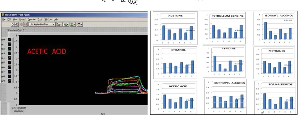
of acetic acid etc. The static response of a sample obtained through DAQ is shown in figure 3.

DATA PREPROCESSING

In order to produce consistent data for pattern recognition system some form of preproceesing of the sensor response is necessary so that the modified response matrix can be fed into pattern recognition (PARC) engine. Preprocessing technique compensates for the variation in the initial condition of the sensor. Techniques in preprocessing include baseline manipulation, linearization and normalization of the sensor output. [14]

Base line manipulation: To remove the drift effect due to the self-instability of the sensor in static response, resulting in bad-reproducibility, base line manipulation is very necessary. This technique transforms the time – dependent sensor signal relative to its baseline. Base line manipulation is done by –

= − …………. (3)

Linearization: The response obtained from a gas sensor for a particular odour will be different at different concentration because of non linearity of MOS gas sensor. To eliminate this drawback linearization technique is implemented on the time independent data-set. Linearization equation is given by—

= ( ) ………. . (4)

Fig 3: Sensor response of a chemical sample at 2378 ppm (60 μL) obtained through LabVIEW.

Normalization: Normalization eliminates the concentration information, e.g. fluctuations in sample injection volume . The normalization equation is given by—

Y/ ₌ Y

∑ Y ……… (5)

After normalization the data is ready for analysing using pattern recognition technique. Some normalized pattern of responses from six sensors for different chemical samples are shown in figure (4). Graphs are plotted by taking

Fig 4: Normalized sensor responses from an array of six sensors for different gas samples

sensor position in x-axis and normalized sensor responses in y-axis. From figure 4, it is observed that the response patterns of the sensors are different for different samples.

IV. CLASSIFICATION OF DATA WITH ANN

Pattern recognition and classification was carried out on the normalized data-set using well known ANNs- namely feed forward multilayer perceptron (MLP). The system hardware was designed with an array of six gas sensors and capable of detecting 9 different gas sample. Thus, the input layer of ANN comprised of 6 input units and 9 output units. Input layer and output layer was connected through a hidden layer of 15 units. The network was implemented using MATLAB. The architecture of the network is shown in Fig (5). Other network parameters are shown in table 1.

After the network had been created and all weights and biases had been randomly initialized, the network becomes ready to be trained using the pre-collected (normalized) data as input. The target data matrix was prepared.

Fig: 5: ANN architecture of MLP network used in designed system(weights are shown only for1 node only)

TRAINING

During training, the weights and biases of the network are iteratively updated to minimize an error function between the desired (target) output(s) and the network output(s). This error function is defined in MATLAB as the mean square error (MSE) which represents the average squared error between the network outputs and the target values.

Training had been done with two target matrices-

1. In the 1st training, the network was trained for a single response obtained from a single sample.

2. In the 2nd training, the network was trained for two different responses obtained for the same sample at different concentration.

x1

x

x

x

Table 1: Network Parameters

Network Type Feed-forward backpropagation

Input layer 6

Hidden layer 15

Output layer 9

Training function TRAINLM

Adaptation learning

function LEARNGDM

Performance function MSE

Fig 6: Training performance of 1st training method

During the training, figure 6 & figure 7 appears. It represents the network performance (in blue) versus the number of epochs. The network performance starts by a large value at the first epochs and due to training the weights are adjusted to minimize this function which makes it decreasing. Moreover, a black constant line is plotted representing the training goal. The training stops when the blue line (network performance) intersects with the black line (training goal).

It is observed from the fig 6 & fig 7 that the both the networks after training approaches to the target matrices. Thus, it can be said that both the networks are well trained and can be used for any application based on it.

SIMULATION:

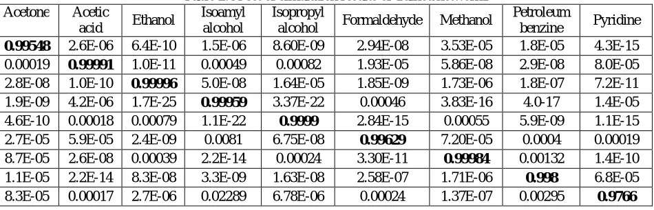
After the network had been trained, a simulation stage was performed to check the network outputs corresponding to a given input. The inputs were the sensor responses obtained from different known samples. For simulation purpose, 18 different responses were collected from different samples at different concentrations. These responses were preprocessed using equation 3, equation 4 and equation 5. Then, the trained networks were simulated with these responses as input to the ANN network. Some of the simulation results are shown in table 2 and table 3. It is observed from the simulation results that trained network 1 and trained network 2 meet the desired (target) value for some of the given samples. (Values in bold letters in simulation results represent the identified targets which are nearly equal to 1).

Table 2: A set of simulation results of trained network1 Acetone Acetic

acid Ethanol

Isoamyl alcohol

Isopropyl

alcohol Formaldehyde Methanol

Petroleum

benzine Pyridine

0.99548 2.6E-06 6.4E-10 1.5E-06 8.60E-09 2.94E-08 3.53E-05 1.8E-05 4.3E-15 0.00019 0.99991 1.0E-11 0.00049 0.00082 1.93E-05 5.86E-08 2.9E-08 8.0E-05 2.8E-08 1.0E-10 0.99996 5.0E-08 1.64E-05 1.85E-09 1.73E-06 1.8E-07 7.2E-11

1.9E-09 4.2E-06 1.7E-25 0.99959 3.37E-22 0.00046 3.83E-16 4.0-17 1.4E-05

4.6E-10 0.00018 0.00079 1.1E-22 0.9999 2.84E-15 0.00055 5.9E-09 1.1E-15

2.7E-05 5.9E-05 2.4E-09 0.0081 6.75E-08 0.99629 7.20E-05 0.0004 0.00019

8.7E-05 2.6E-08 0.00039 2.2E-14 0.00024 3.30E-11 0.99984 0.00132 1.4E-10

1.1E-05 2.2E-14 8.3E-08 3.3E-09 1.63E-08 2.58E-07 1.71E-06 0.998 6.8E-05

8.3E-05 0.00017 2.7E-06 0.02289 6.78E-06 0.00024 1.37E-07 0.00295 0.9766

Fig 7: Training performance of 2nd training method

0 5 10 15 20 25 30

10-5 10-4 10-3 10-2 10-1 100

30 Epochs

T

ra

in

in

g

-B

lu

e

G

o

a

l-B

la

c

k

Table 3: A set of simulation results of trained network2

Acetone Acetic

Acid Ethanol

Isoamyl Alcohol

Isopropyl Alcohol

Formaldehyd

e Methanol

Petroleum

Benzine Pyridine

0.91258 0.0050 0.00568 0.03907 0.007771 0.0011196 0.038644 0.10829 0.00094 3.1E-06 0.9315 9.3E-05 0.001619 2.63E-05 0.0035578 0.021707 2.05E-07 0.01197 7.9E-06 6.3E-6 0.95162 1.04E-05 0.024073 4.06E-06 7.59E-05 2.44E-05 1.49E-08 0.00241 0.0002 3.9E-05 0.96149 0.018689 0.0089038 7.88E-05 6.89E-05 1.45E-05 0.00165 0.0284 0.06112 8.56E-05 0.96747 7.56E-07 0.040799 0.0001647 0.00538 0.00287 0.0437 0.00108 0.007706 7.09E-09 0.97063 0.012422 0.0008693 0.01220 0.00215 0.0170 0.00124 3.50E-05 4.57E-05 0.00032036 0.95082 0.0058832 0.00077 0.04394 1.3E-5 0.00228 4.23E-06 0.002277 0.00014789 0.000235 0.94254 0.00874 0.00013 0.0086 1.6E-06 7.04E-06 2.62E-06 0.021131 7.32E-06 0.0012162 0.97295

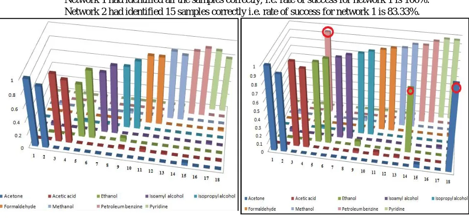
A graphical plot of simulated results of trained network 1 is shown in fig.8. From the graph it is observed that for one series of data- set only one output is nearly equal to the target i.e 1. Here, out of 18 samples, all the samples can be classified correctly.

A graphical plot of simulated results of trained network 2 is shown in fig.9. From the graph it is observed that for the series of data-set 5, 14 and 18, instead of only one output, two outputs are nearly equal to the target i.e. 1. So, with trained network 2, out of 18 samples only 15 samples can be classified correctly.

Comparing the simulated results of the two trained networks, it was found that out of 18 responses –

 Network 1 had identified all the samples correctly, i.e. rate of success for network 1 is 100%.

 Network 2 had identified 15 samples correctly i.e. rate of success for network 1 is 83.33%.

Fig 8: Simulation of trained network1 with 18 samples (All the samples meet the target values correctly)

So we can conclude with that it is better to use the weights and biases values of trained network 1 for implementing the ANN structure in microcontroller. The weights to the input layer and hidden layer are shown in table 2 & 3. The biases to the input layer and hidden layer are shown in table 4 & 5.

V. SAMPLE IDENTIFICATION

The sample identification system comprises a sensor chamber, two micro pumps, microcontroller- embedded with ANN, LCD and power supply. (Figure 10)

Fig 10: Block diagram of Sample Identification process

At first the sensors are heated by a 5V power supply, while the pump is ON. When a base line voltage of air is obtained, the unknown chemical is supplied to the inlet of the pump1. The pump pushes the sample around the inlet into the sensor chamber. The responses obtained from the sensors are fed to the analog input of the microcontroller. The microcontroller then identifies the sample using pattern recognition algorithm and display the name of the gas in the LCD. When the detection process is completed the sensors are cleaned properly with sufficient fresh air. Detailed description of each block is depicted below-

A. Sensor chamber

To be able to get nice pattern for a wide range of odorants and to classify them correctly, the response of each sensor in the array should be different. The sensor array used in the portable E-nose was comprised of six TGS gas sensors (figure 11) namely: TGS 826, TGS 2600-303A2, TGS 2610, TGS 2600-9N4TF, TGS 2611 and TGS 825 as commercially available from Figaro Engineering Inc. The gas sensors responses are fed to 6 analog input ports of microcontroller.

B. Implementation of ANN in microcontroller

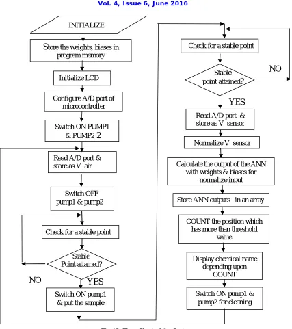
ANN was implemented in PIC 18F452 microcontroller. As mentioned before the input layer had 6 inputs which were the sensor responses obtained by reading the analog ports of the PIC microcontroller. These responses were normalized and then used as an input to the ANN module. The flow chart of the system is shown in figure 12.

Fig 12: Flow Chart of the System

The weights (table 4 and table 5) and the biases (table 6 and table 7) for layer 1 and layer 2 were collected from the already trained network. These were stored in program memory of the microcontroller. The resistance of the air (table 8) was also stored in program memory to remove the baseline manipulation of the sensors (equation 3). Microcontroller was programmed in MicroC to implement the ANN structure. The outputs of the ANN module were calculated using standard equations of ANN shown in equation 6. The activation function used was logsigmoid (equation 7). The outputs of the 1st layer were used input to the 2nd layer and then 2nd outputs were calculated using the same equations.

= ∑ + = + +⋯+ + ….. (6) = ( ) = _{( )} …. (7)

Initialize LCD

Switch ON PUMP1 & PUMP2 2

Read A/D port & store as V_air

Switch OFF pump1 & pump2

Check for a stable point

Stable

NO

_YES

Read A/D port & store as V_sensor INITIALIZE

Store the weights, biases in

Store ANN outputs in an array

COUNT the position which has more than threshold

value

Switch ON pump1 & pump2 for cleaning Display chemical name

depending upon COUNT

Calculate the output of the ANN with weights & biases for

normalize input Configure A/D port of

microcontroller

Switch ON pump1 & put the sample

Normalize V_sensor

Stable

point attained?

YES

Where, wi = weights to different layers, xi= normalized inputs to the layers, b= bias.

Table 4: Weight to layer 1

-22.146 -10.846 8.858 29.773 41.600 10.781

-5.917 27.801 -15.271 88.000 22.322 35.163

-15.979 48.041 -2.936 -41.601 24.523 -26.305

24.230 31.230 2.987 -47.953 -16.952 -33.506

21.150 -25.562 -26.877 41.380 6.189 -13.497

-9.828 39.372 16.164 0.620 12.834 50.784

-10.687 12.697 -32.222 -52.066 27.055 25.831

-19.065 -34.733 -16.092 15.008 -38.681 15.583

-13.753 -29.451 16.437 65.721 -34.291 28.145

16.870 33.438 -14.614 82.170 27.449 -3.425

-6.866 47.616 -15.776 -11.364 -31.359 -28.328

6.234 13.709 -9.354 -21.734 -59.824 -27.177

-14.835 -13.860 -1.466 110.634 -18.515 30.343

18.764 -39.247 -0.033 35.493 43.451 15.758

-14.665 -7.008 3.774 103.748 -28.054 16.603

From the nine outputs of the ANN structure, positions which had values higher than 0.9 (almost equal to 1) were determined. Depending upon the position of the threshold value (0.9), the identified chemical name was displayed in LCD. Chemical names depending on the position are shown in table 9.

Table 9: Identification of chemical depending upon position of threshold value in the calculated ANN output

Position of

threshold value 1 2 3 4 5 6 7 8 9

Name of

chemical Acetone

Acetic

Acid Ethanol

Isoamyl Alcohol

Isopropl

Alcohol Formaldehyde Methanol

Petroleum

Benzine Pyridine

Steps to operate the softwere

 Switch on the power supply of the sensor and apply a heater voltage around 4.9 V

 Wait for almost 15 minutes so that the heater coils get sufficiently heated.

 After that switch on the microcontroller and the LCD.

 When the LCD will display “ put the sample ”, place the sample to the inlet of the pump1.

 After few moments the chemical will be identified and name of the chemical will be displayed in LCD.

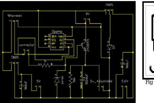
C. Power supply:

A power supply circuit (figure 13) is designed to produce three different sources of supply voltages such as- (a) Regulated 5V supply to operate microcontroller, LCD and circuit voltage of the sensors. This is done using a 7805

Table 5: Weight to layer 2

2

-4.6 -6.5 6.53 -9.8 -5.4 6.69 0.16 -9.9 4.87 5.6 -1.4 14.27 -3.3 -8.64 -10

3.16 3.14 4.15 2.13 -0.8 -5.1 -17 -3.5 3.14 0.3 0.87 -0.89 0.8 0.116 1.5

-2.3 6.5 -0.7 0.32 -4.1 -1.2 6.14 -4.1 4.27 6.8 -0.9 -12.1 -2.8 -12.5 -4.6

-1.5 -7.2 -1.8 6.47 -4.1 -4.1 0.11 -4.7 -5.8 1.9 2.3 0.153 -2.7 -3.52 -2.8

-1.9 -3.2 4.19 -3.3 -5.1 7.8 -2.8 -3.7 -11 -2.1 -4.6 -0.75 4 16.26 15

-6.7 7.65 0.53 -10.8 9.83 -7.18 13.3 -5.9 -4.6 0.3 6.37 2.722 0.8 -4.75 -5.5

0.04 -0.7 -2.8 -0.8 -3.9 -1.33 -1.9 1.99 0.47 0.7 6.41 0.903 3.2 -6.37 3

-0.4 2.49 -4.3 -1.4 -7 3.68 0.34 8.86 3.08 -8.1 -6 1.127 -2 2.393 -0.4

0.39 1.97 -6 -0.64 2.74 -6.33 -2.8 4.26 3.96 5 -5.9 -2.91 1.7 2.974 -2.2

Table 7: Bias to Layer2

-11.1764 -2.1201 -5.3612 7.073 -6.3274 -8.3138 -2.6916 -2.6184 -5.7921

Table 8:

voltage regulator and capacitor. (b) 5.6V supply to run the micro-pumps. This is achieved by 5V regulator (3-pin type) has its ground leg attached to backward-connected 1N4005 diode. The other end of the diode is grounded. (c) Adjustable 5V supply to feed heater voltage of the using emitter follower circuit with 2N3055 transistor and 5.6V zener diode. A 10k preset is connected to the circuit through supply to vary the output voltage. The variable end of the preset is connected to a non inverting op-amp which acts as a voltage follower. This will supply the current to the loads instead of delivering from the supply. Output of the op-amp is then connected to the base of the 2N3055 through a resistor. The PCB design of the power supply circuit is shown in figure 14.

Fig 13: Power supply circuit designed in DipTrace

VI. RESULTS AND DISCUSSION

After implementing the ANN on the microcontroller, it was tested for 25 chemical samples at different concentrations. Out of these samples, the designed portable E-Nose was capable of detecting 24 samples correctly irrespective of their concentrations. The name of any identified sample is displayed on the LCD panel of the system (figure 15).

Fig 15: A Sample is identified and the name is displayed in LCD

Microcontroller results:

Total no. Of sample tested = 25 Correctly identified = 24 Target missed =1 Success rate= 96 %

The missed target condition can be justified with the fact that the sensors used in identification process need proper heating to response in a unique pattern to a particular stimuli. Moreover after every identification process they need proper cleaning so that there is no residual left.

VII. FUTURE SCOPE

A quite accurate and capable E-nose system and training algorithm is developed during this project work; nevertheless, further work is needed to access the long-term reliability of the E-nose system. The use of a commercial headspace auto sampler can be very useful with thee sampling process and thus system performance can be improved. This will result in a system that is more suitable for commercial application for continuous monitoring.

VIII. REFERENCES

1. Gardner, J.W. and Baktlett, P. N., “A brief history of electronic noses”, Sensors and .Actuators B, Chem, 18-19, pp. 21 1-220., 1990.

2. Gardner, J.W., Guha, P.K, Florin Udrea, and James A. Covington “CMOS Interfacing for Integrated Gas Sensors: A Review” ieee sensors journal, vol. 10, no. 12, december 2010.

3. Wise, K. D., “Integrated sensors – interfacing electronics to a non-electronic world,” Sens. Actuators, vol. 2, no. 3, pp. 229–237, 1982. 4. Gardner, J.W., Hines, E. L., and Wilkinson, M., “Application of Artificial Neural Networks to an Electronic Olfactory System,” Measurement

Science and Technology, vol. 1, no. 5, pp. 446-451,May 1990.

5. Moriizumi, T., Nakamoto, T., and Sakuraba, Y., “Pattern Recognition in Electronic Noses by Artificial Neural Network Models,” in sensors and Sensory Systems for an Electronic Nose, J.W. Gardner and P.N. Bartlett, Eds. Amsterdam, The Netherlands, Kluweer Academic Publishers, pp. 217-236.,1992.

6. Hines, E. L., Llobet, E., and Gardner, J. W., “Electronic noses: a review of signal processingTechniques” IEE Proc. – Circuit Devices Syst . ,Vol 146. No. 6, December 1999

7. Baltes, H. and Brand, O., “Progress in CMOS integrated measurement systems,” in Proc. 16th IEEE Instrum. Meas. Technol. Conf., Venice, Italy, pp. 54–59.,1999.

8. Wise, K. D. and Najafi, K., “Microfabrication techniques for integrated sensors and microsystems,” Science, vol. 254, no. 5036, pp. 1335–1342, Nov. 1991.

9. Hagleitner, C., Hierlemann, A., Lange, D., Kummer, A., Kerness, N., Brand, O., and Baltes, H., “Smart single-chip gas sensor microsystem,”

Nature, vol. 414, no. 6861, pp. 293–296, Nov. 2001.

10. Hierlemann, A., Lange, D., Hagleitner, C., Kerness, N., Koll, A., Brand, O., and Baltes, H., “Application-specific sensor systems based on CMOS chemical microsensors,” Sens. Actuators B: Chem., vol. 70, no. 1–3, pp. 2–11, Nov. 2000.

11. Gardner, J. W., Cole, M., and Udrea, F., “CMOS gas sensors and smart devices,” in Proc. IEEE Sensors, Orlando, FL, pp. 721–726, 2002. 12. Joo, S., and Brown, R. B., “Chemical sensors with integrated electronics,”Chem. Rev., vol. 108, no. 2, pp. 638–651, Feb. 2008.

13. Gardner, J. W., Hines E. L., and Wilkinson M., “Application of artificial neural networks to an electronic olfactory system”, Meas. Sci. Technol. pp- 446-451.,1990 .

14. Uyanik A. and Tinkiliç. N, “Preparing Accurate Standard Gas Mixtures of Volatile Substances at Low Concentration Levels”, Chem. Educator, 4, 141– 143,1999.

BIOGRAPHY

Namrata Kataki is an assistant professor in the Electronics and Communication department, Girijananda Chowdhury Institute of Management & Technology (GIMT), Guwahati. She received M.Tech degree from Tezpur University in the year 2012. Her research interests are microcontroller, embedded system.