Comparison of Various Transfer Functions
for Resilient Back-Propagation Algorithm
Mahua Ghosh 1*, Ayan kumar Bhar 2, Adwitiya Mullick 3, Bishwarup Biswas 4, Dr. Monal Dutta 5
Student, Department of Chemical Engineering, Calcutta Institute of Technology, Howrah, West Bengal, India1,2,3,4
Associate Professor, Department of Chemical Engineering, Calcutta Institute of Technology, West Bengal, India 5
ABSTRACT: A three layer artificial neural network was constructed to predict the phenol adsorption capacity through batch adsorption. The basic network architecture consisted of five input parameters and one output parameter. Various input parameters such as, solution pH (2 -8), adsorbate concentration (30 – 120 mg/L), adsorbent concentration (1- 3 g/L), contact time (5 – 120 min) and temperature (30 – 50 °C) were considered for this purpose whereas the phenol removal capacity (mg/g) was taken as the output variable. Resilient back-propagation algorithm was applied to model the adsorption process and it was found that “satlin” transfer function with five neurons in the hidden layer yield best result with an appreciable regression coefficient (R2 = 0.999) value and minimum mean squared error (MSE = 0.00004) value.
KEYWORDS:ANN, Back-propagation, Adsorption, Modelling.
I. INTRODUCTION
The artificial neural network (ANN) is a powerful simulation tool generally used to model several nonlinear functions. Over the past few decades, ANN has been successfully employed in various fields including adsorption [1]. The prediction of system output by ANN is generally based on the performance of human brain [2]. The most commonly used ANN is multilayered feed-forward neural network which comprises of an input layer, a hidden layer and an output layer. The response in this network moves from one layer to another in a forward direction. The input dataset is subdivided into three parts training, test and validation in a ratio of 3:1:1. In the training stage, the input variables are multiplied with a certain weight and then the product is summed up with the biases in order to produce the desired output. The values of respective weights and biases are updated after each iteration by a certain value to enhance the system performance. The test data set are used to predict the system performance whereas, the validation set confirms no over fitting of the network [3].Various algorithms are generally used to train the network such as, Levenberg– Marquardt back-propagation(trainlm), resilient back-propagation (trainrp), scaled conjugate gradient back-propagation (trainscg), Polak-Ribiére update (traincgp) and gradient descent propagation among which resilient back-propagation algorithm is able to produce comparatively faster convergence of the network objective function. Therefore, in the present time ANN is successfully used to predict the efficiency of various physical systems.
The phenolic compounds are most commonly detected in various industrial waste streams including oil refineries, plastics, synthetic resins, leather, paint, coal gas oven plants etc [4–5]. the presence of phenolic compounds even in a small concentration in the waste streams divulge various toxic effects on fish and as well as on human beings including liver and kidney damage, headache, tissue erosion, paralysis of the central nervous system and vomiting [6-7]. Therefore, it has become very necessary to remove phenol from wastewater before discharging it in the water bodies. In the present investigation, a three layer feed-forward neural network with resilient back-propagation algorithm is used to predict the phenol adsorption characteristics onto the surface of chemically modified adsorbent.
II. EXPERIMENTAL
The adsorbent was prepared by treating the natural clay collected from local river basin by zinc acetate dihydrate. The detailed procedure was described in previous work by Bhar et al. (2017) [8].
III.STRUCTURE OF ANN NETWORK
The neural network consists of an input layer, a hidden layer and one output layer. The number of neurons in the input layer is equal to the number of input parameters and number of neuron in the output layer is equal to the number of output parameter. These neurons are connected with each other with particular weight and bias functions. The optimum number of neurons in the hidden layer is generally decided by varying the number of neurons and transfer functions in the hidden layer. The commonly used transfer function in the hidden layer of ANN is sigmoid function. In the simulation process of ANN, the weight functions are updated every time in order to minimize the error. The basic construction of a neural network can also be expressed as a two dimensional matrix W between input and hidden layer with the entry variable of kth layer and ith element (wki), whereas, the weight wʹij is considered as the (i,j)th entry variable
in a N×M weight matrix W between hidden and output layer. Therefore, output in the hidden layer can be calculated as the weighted sum of the neuron's inputs and is given by [9]
K k k ki ii f u f w x
v
1
) (
the output layer is expressed as
N i i ij ij f u f wv
y
1
) (
Similarly, the objective function is also determined by summing up all the elements in the output layer as
M j j j t y E 1 2 ) (Once the objective function is defined then the update equations for input to hidden layer and hidden to output layer has to be calculated. For this purpose, gradient of the objective function with respect to wʹij (∂E/∂wʹij) needs to be
determined first. Here, the derivative of objective function (E) with respect to the logistic function (yʹj) has to be taken
and then the derivative of yj with respect to wʹij (input uʹj) has to be considered as below:
j j j ij j j j j ij t y y E where w u u y y E w E ,
Therefore, the updated weight function is calculated as
i j j j j oldij
newij w y t y y v
w ( ) (1 )
After making the appropriate substitutions we arrive at the gradient
k i i M i j ij j j j j i k x v v w y y t y w E ) 1 ( ] ) 1 ( ) [(
And the update equation becomes
k i i M i j ij j j j j oldki ki
new w y t y y w v v x
w
[( ) (1 ) ] (1 )
This process is known as back-propagation because we begin with the final output error yj − tj for the output neuron j
IV.DEVELOPMENT OF ANN MODEL
A three layer feed-forward back-propagation neural network was used to predict the phenol adsorption capacity. In the present study, resilient back-propagation algorithm with different transfer functions such as tangent sigmoid, saturated linear and positive linear transfer in the hidden layer were applied to predict the adsorptive removal of phenol. The numbers of neurons in the hidden layer were varied from 5 to 11 for various transfer functions. The input parameters were solution pH, initial concentration, adsorbent dose, contact time and temperature and the phenol removal capacity was the output variable. The range of the input parameters was discussed in detail in a previous literature by Biswas et al., (2017) [10]. Neural network mathematical software of version R2008a was used to model the adsorption process.
V. RESILIENT BACK-PROPAGATION
Among the all the back propagation algorithm resilient back-propagation is regarded as the best algorithm because of high convergence speed, robustness of the developed model and high accuracy [11]. The gradient of the given function gradually decreases to zero as the size of the input gets increased. But this small change in the gradient causes insignificant change in weights and biases which in turn increases the computational time by moving the function far from the optimal region. The resilient back-propagation (Rprop) training algorithm is used to overcome this limitation as magnitude of the derivative functions is
found to have no effect on the weight update. The direction of weight update can only be determined through the sign change in the derivative function. The step size of the derivative functions are increased by a constant factor delta_inc when the derivative of the objective function is expressed as a function of weight values and they carry same sign for two successive iterations. On the other hand, the value of the objective function is decreased a constant factor delta_dec when there is a sign change between two successive derivatives. In case of no change in derivative value, the update value remains the same. The size of step change in the weight function generally is kept low in case of small oscillation.
VI.RESULTS AND DISCUSSION Optimization using ANN structure
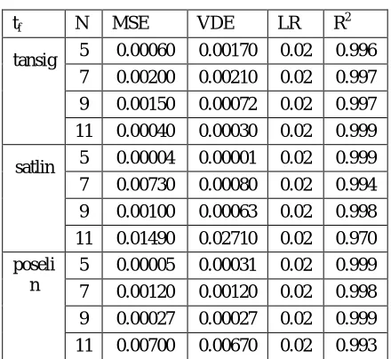
In order to investigate the adsorption process resilient back-propagation algorithm with different transfer functions such as "tansig", "poselin" and "satlin" were applied in the hidden layer. The comparison of the transfer functions are shown in Table I. The performance of the neural network is highly dependent on the number of neurons in the hidden layer. Increasing the number of neuron in the hidden layer helps to enhance the network performance but use of too many neurons in the hidden layer leads to over fitting of the given network [12]. Therefore, the number of neurons has to be optimized for useful training of the given network. The numbers of neurons were varied from 5 to 11 in the hidden layer.
Table I: The comparison of various networks
tf N MSE VDE LR R2
tansig 5 0.00060 0.00170 0.02 0.996 7 0.00200 0.00210 0.02 0.997 9 0.00150 0.00072 0.02 0.997 11 0.00040 0.00030 0.02 0.999
satlin 5 0.00004 0.00001 0.02 0.999 7 0.00730 0.00080 0.02 0.994 9 0.00100 0.00063 0.02 0.998 11 0.01490 0.02710 0.02 0.970 poseli
n
It is evident from Table I that “satlin” transfer function exhibits better simulation result with high value of regression coefficients (R2 = 0.999 ) and comparatively lower mean squared error (MSE) and validation error (VDE). According to Table I the smallest MSE was found to be 0.00004 and the VDE was found to be 0.00001. The relationship between the MSE and the number of neurons in the hidden layer is shown in Fig. 1. It can be seen from Fig. 1 that the minimum MSE value is resulted for 5 numbers of neurons in the hidden layer and the corresponding error values are increasing with increase in number of neurons from 5 to 11. The similar trend was also found in the previous literature [13].
Fig. 1. Plot of MSE value with number of iterations
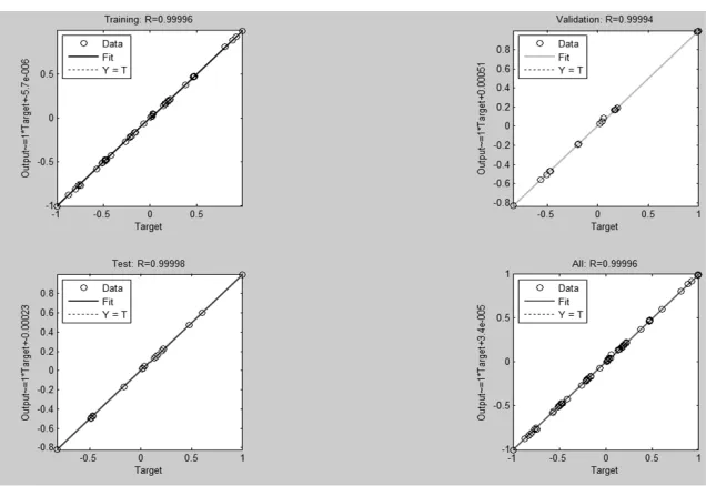
The output and target values are compared for training, test and validation purpose for “satlin” transfer function (Fig. 2). It is evident from Fig. 2 that the models generate a better fit with high value of regression coefficient (R2 = 0.999 ).
VII. CONCLUSION
In the present investigation, a three layer artificial neural network had been developed to predict the phenol adsorption capacity. For this purpose, resilient back propagation algorithm with “tansig”, “poselin” and “satlin” transfer function were applied with varying numbers of neuron (5 – 11) in the hidden layer. The performance of the developed network was judged in terms of MSE and VDE. It was found that “satlin” transfer function with 5 numbers of neurons in the hidden layer produced minimum MSE (0.00004) and VDE (0.0000) values.
REFERENCES
[1] N. Sundaram, "Training neural networks for pressure swing adsorption processes.", Ind. Eng. Chem. Res., vol. 38, no. 11, pp. 4449–4457, 1999.
[2] B.B. Ekici, U.T. Aksoy, "Prediction of building energy consumption by using artificial neural networks., Adv. Eng. Softw., vol. 41, no. 2, pp. 141–147, 2010.
[3] L. Cavas, Z. Karabay, H. Alyuruk, H. Dogan, G.K. Demir, "Thomas and artificial neural network models for the fixed-bed adsorption of methylene blue by a beach waste Posidonia oceanica (L.) dead leaves.", Chem.Eng. J., vol. 171, no. 2, pp. 557–562, 2011.
[4] P. Canizares, M. Carmona, O. Baraza, A. Delgado, M.A. Rodrigo, "Adsorption equilibrium of phenol onto chemically modified activated carbon F400.", J. Hazard. Mater., vol. B131, no. 1-3, pp. 243, 2006.
[5] S. Mukherjee, S. Kumar, A.K. Misra, M. Fan, "Removal of phenols from water environment by activated carbon, bagasse ash and wood charcoal.", Chem. Eng. J., vol. 129, no. 1-3, pp. 133, 2007.
[6] H. Li, M. Xu, Z. Shi, B. He, "Isotherm analysis of phenol adsorption on polymeric adsorbents from nonaqueous solution.", J. Colloid. Interf. Sci., vol. 271, no. 1, p. 47, 2004.
[7] R. Qadeer, A.H. Rehan, "A study of the adsorption of phenol by activated carbon from aqueous solutions.", Turk. J. Chem., vol. 26, p. 357, no. 3, 2002.
[8] A.K. Bhar, A. Mullick, B. Biswas, M.Ghosh, P. Sardar, M. Dutta, “Optimization of phenol adsorption characteristics through central composite design,” International Journal of Emerging Technology and Advanced Engineering, vol. 7, no. 5, pp. 18-21, 2017.
[9] M.R. Dashtbayazi, A. Shokuhfar, A. Simchi, “Artificial neural network modeling of mechanical alloying process for synthesizing of metal matrix nanocomposite powders”, Material Science and Engineering A, vol. 466, no. 1-2, pp. 274-283, 2007.
[10] B. Biswas, A.K. Bhar, A.Mullick, M. Ghosh, M. Dutta, “Scaled Conjugate Back-Propagation Algorithm for Prediction of Phenol Adsorption Characteristics”, International Journal of Engineering and Advanced Technology, vol. 6, no. 5, pp. 155-158, 2017.
[11] M. Riedmiller, H. Braun, “A direct adaptive method for faster backpropagation learning: The RPROP algorithm”, Proc. IEEE Int. Conf. On Neural Network, pp. 586-591, 1993.
[12] M. Saemi, M. Ahmadi, A. Yazdian Varjani, “Design of Neural Networks Using Genetic Algorithm for the Permeability Estimation of the Reservoir,” J. Petrol. Sci. Eng., vol. 59, no. 1-2, pp. 97, 2007.