Probabilistic Analysis of Failure of the Steam Distribution Device

(1)

18th International Conference on Structural Mechanics in Reactor Technology (SMiRT 18) Beijing, China, August 7-12, 2005 SMiRT18-M02-2

PROBABILISTIC ANALYSIS OF FAILURE OF THE STEAM

DISTRIBUTION DEVICE

Gintautas DUNDULIS

Laboratory of Nuclear Installation Safety,

Lithuanian Energy Institute, 3 Breslaujos str.,

LT-44403 Kaunas, Lithuania

Phone:+370 37 401918, Fax:+370 37 401918

E-mail: [email protected]

Ronald F.

KULAK

RFK Engineering Mechanics

Consultants, USA

Robertas ALZBUTAS

Lithuanian Energy Institute, Lithuania

Sigitas

RIMKEVICIUS

Lithuanian Energy Institute, Lithuania

ABSTRACT

The parameters used in structural integrity analyses are approximate and have distributions associated with their uncertainties. The material parameters, structural geometry and the applied loads (pressure, force, and temperatures) are all uncertain. These random effects should be incorporated into the analysis in order to have a more realistic estimation of the range of the structural response. The probabilistic analysis of failure of the steam distribution headers and their connections to the vertical vent pipes during a loss-of-coolant accident is the main subject of this paper.

The codes ProFES and NEPTUNE are used for probabilistic analysis of failure of the steam distribution headers and their connections with the vertical vent pipes. ProFES is a probabilistic analysis system that allows designers to perform probabilistic finite element analysis (FEA) in a 3D environment that is similar to modern deterministic FEA. In this study ProFES is coupled to the deterministic finite element code NEPTUNE. The coupled code approach simplifies the modeling of uncertainties and evaluates the effect of these uncertainties on model and system reliability. Monte Carlo Simulation and Response Surface Methods were used for probabilistic analyses of the steam distribution headers and their connections with the vertical vent pipes.

Keywords: Finite Element Method, Probabilistic Finite Element Analysis, RBMK-1500, Structural

Integrity Evaluation.

1. INTRODUCTION

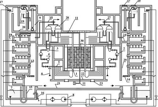
The nuclear reactors of the Ignalina NPP are RBMK-1500 type reactors. These reactors do not possess the conventional Western containment. Instead, Ignalina NPP has a pressure suppression type confinement, which is referred to as the Accident Localization System (ALS). The ALS prevents the release of the radioactive material from the NPP to the environment during a loss-of-coolant accident. The ALS of the Ignalina NPP consists of a number of interconnected compartments. The schematic view of the Ignalina NPP ALS and the location of main components of the main circulation circuit (MCC) are presented in Fig. 1.

(2)

function. Because of the uncertainties in material properties, structural geometry and loadings, it is necessary to determine through probabilistic analyses if a combination of the problem parameters, as defined by probability distributions, could lead to failure of the SDD and then determine the probability of failure.

17

9 10 28 11 27

25 26

24

2

29

14 23

22 11 1 6

5 3 4 12

13 18

30

21 16 15 7

20 19

8

Fig. 1.

The scheme of Ignalina NPP ALS and location of main components of MCC: 1 – fuel

channel, 2 – main circulation pumps, 3– suction header, 4 – Pressure Header, 5 – GDH, 6

– ECCS headers, 7 – hot condensate chamber, 8 – CTCS pumps and heat, 9 – discharge

pipes section, 10 – pipes from MSV and BRU-B, 11 – pipes from reactor cavity, 12 –

condensing pools, 13 –steam distribution headers, 14 – BSRC sprays, 15 – S/traps

between HCC and BSRC, 16 – BSRC vacuum breakers, 17 – air removal corridor sprays,

18 – air venting channel, 19 – gas delay chamber tank, 20 – gas delay chamber, 21 –

reinforced compartments, 22 – down hatches, 27 – MSV and BRU-B, 28 – drum

separators, 29 – BSRC, 30 – reactor.

The probabilistic analysis of failure of the steam distribution headers and their connections to the vertical vent pipes during a loss-of-coolant accident was presented in this paper. This analysis was performed using a commercial probabilistic code, ProFES (PROFES), and a proprietary finite element code, NEPTUNE (Kulak, 1988). The two codes are coupled through the pnglue code (Kulak, 2003). Three-dimensional finite element models of the SDDs were developed and analyzed for combined thermal and pressure loadings. Random variables and their distributions were selected and the response variables were processed to determine the effect of uncertainties on model and system reliability. Monte Carlo Simulation and Response Surface Methods were used for probabilistic analyses of the steam distribution headers and their connections with the vertical vent pipes.

2. MODEL FOR PROBABILISTIC ANALYSIS OF FAILURE OF THE STEAM DISTRIBUTION HEADERS AND THEIR CONNECTIONS WITH THE VERTICAL VENT PIPES

The SDD consist of 2, 3 or 4 (pertains to length) prefabricated elements. The construction of one prefabricated element and the cross-section of a SDD is presented in Fig. 2, a. The main parts of the SDD are the steam distribution header (SDH) and the vertical steam nozzles (see Fig. 2, a). The SDH is a horizontal cylinder with an outside diameter of 806 mm, a wall thickness of 3 mm. The vertical steam nozzles are boxes in the shape of parallelepipeds. The cross-section of this box is presented in Fig. 2, b. Section 2-2 has the following dimensions: length 1000 mm, width 50 mm, wall thickness 3 mm, heights 1375 mm. A hood is around the vertical steam nozzle to provide an air cushion. The dimensions of the cross-section of the hood are 1026x82 mm. The nozzles are installed in pairs. The distance between these nozzles is 600 mm across the longitudinal axis (Fig. 2, a - section 1-1). The connection of the SDH and the vertical steam nozzle is presented in Fig. 2, b - section 3-3. The vertical steam nozzle is separated into 5 channels. The thickness of the dividing walls is 3 mm.

(3)

a) b)

Fig. 2. The construction of one part of SDD: a – general view of SDD, b - cross-section of

vertical steam nozzle and joining of the SDH with nozzles

The connectors of the vertical steam nozzles were modeled using 3D beam elements developed by Belytschko, et al. (Kulak, 1988). Beam elements are two-node members allowed arbitrary orientation in the 3-D (three-dimensional) X, Y, Z space. An additional node (K-node) is required to define the element orientation. It is a general six (6) degree of freedom element (i.e., three global translation and rotational components at each end of the member). The beam element provides moment, torque and force information. The 3-D beam element is a three-dimensional uniform cross-section element capable of performing large deformations and elasto-plastic analysis of general beam-frame problems. The cross-section change of shape is not accounted for in any analysis. Externally, the beam has six degrees of freedom - three displacements and three rotations. It supports full 3-D translation and rotation motions. The 3-D beam element is often used in analyses when bending, torsion and stretching behavior occurs with large deformations and/or material nonlinear effects.

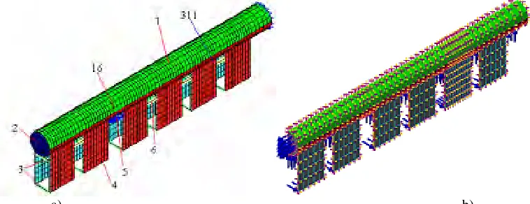
The SDD FE model prepared for probabilistic analysis is shown in Fig. 3a. Due to symmetry, only one-half of the FE model of the SDD was used for probabilistic analysis. The half-part of the SDD header pipe, the half-part of the SDD pipe end, the vertical vent pipes and the connectors (the connectors are not presented in Fig. 3b) are included in the model for probabilistic analysis. The numbers of the elements that were used for determination of the failure probability of the SDD are presented in Fig. 3a.

a) b)

Fig. 3. Combined model for finite element analysis of the SDD 8500x1600, a – all the FE model,

b – one-half part of the FE model: 1 – SDD pipe, 2 – SDD pipe end, 3 – cross connectors,

4 – vertical vent pipes, 5 - SDD supports constrains, 6 – longitudinal connectors; the

element numbers selected for probabilistic analysis: 16 - the SDH pipe element adjacent

to the SDD header support constrains, 311 - the SDH pipe element adjacent to the

connection of the SDD header and vertical vent pipe.

3. PROBABILISTIC ANALYSIS METHODS USED IN ANALYSIS

(4)

Mechanics Group of Applied Research Associates Southeast Division, located in Raleigh NC (Cesare, 1999). ProFES allows quick development of probabilistic models from the model executables, analytical formulations, or finite element models. It is possible to use ProFES independently to perform probabilistic simulations using functions internal to ProFES or functions that can be manually typed in. ProFES can be used as an add-on to the modeled executables, so it is possible to perform probabilistic studies using the deterministic models. The NEPTUNE code is used for structural integrity analysis of the SDD. Since NEPTUNE input cannot be directly imported into the ProFES code, a special ProFES/NEPTUNE translator (pnglue) was developed to address this issue (Kulak, 2003). The translator, which is written in Perl, has been developed to seamlessly exchange information between NEPTUNE and ProFES.

The following methods for numerical probabilistic analysis are included in ProFES:

• Monte Carlo Simulation (MCS) generates samples of each random variable, and runs the deterministic model at each combination. Statistics and probabilities are determined by a simple statistical analysis of the results.

• Importance Sampling is used to execute an importance sampling analysis. This method differs from MCS in that it only samples in a specific region in order to reduce the number of simulations. The method implemented here samples in the region around the most probable point.

• The First Order/Second Moment method finds the gradients of the limit state function at the mean values of the random variables, fits a linear response surface at this point, and estimates mean and standard deviation of response.

• The First Order Reliability Method (FORM) searches the input variables for the combination that is most likely to cause failure (this point is often referred to as the design point or the most probable point, MPP). It then fits a linear surface at the MPP and uses this surface (along with transformations for any non-normal random variables) to compute probabilities. A variant of this method is SORM; wherein a second order surface is fitted at the MPP.

• The RS/MCS method fits a response surface about the mean of the random variable and then computes statistics of response variables and probabilities for each limit state using MCS.

• The Adaptive Response Surface. This method is the same as the RS/MCS method except that the surface is fitted about the MPP.

The MCS and FORM methods are not possible to use in the probabilistic analysis of the SDD model. One run of the SDD FE model using the NEPTUNE code takes approximately 8 hours. If MCS is used for probabilistic analysis, 100 runs will require about 800 hours, i.e. more that one month. Note, the simulation number of 100 is very small for probabilistic analysis. The simulation number of 1000 (approximately) is needed for probabilistic analysis using FORM.

The RS/MCS method was employed for the determination of response surfaces (dependence functions) of failure of the steam distribution headers and their connections with the vertical vent pipes. The probability of this failure was calculated by MCS method using response surfaces (dependence functions).

The results from thermal hydraulic transient analysis were used to define the dynamic loading used in the structural integrity analysis. The lumped-parameter code COCOSYS V2.0v0 (COCOSYS, 2001) is employed for the analysis of the thermal-hydraulic parameters in the compartments of the ALS. The loads obtained from the thermo hydraulic analysis are about 10 % uncertain. Therefore, it is important to estimate the dependence of the failure probability (or impact to neighboring pipe or wall) on the uncertainty in loading. The RS/MCS method was used for determination of such a relation expressed by the probability-loading function.

4. PROBABILISTIC ANALYSIS RESULTS OF FAILURE OF THE STEAM DISTRIBUTION HEADERS AND THEIR CONNECTIONS WITH THE VERTICAL VENT PIPES

The RS/MCS method was used for determination of a probability function for probabilistic analysis of failure of the steam distribution headers and their connections with the vertical vent pipes. The random variables and limit states selected for probabilistic analysis are presented in the following sub-sections

4.1 Selected Random Variables forAnalysis

(5)

1. Mechanical properties:

Austenitic steel of SDD pipes – thermal expansion coefficient, Young’s modulus at different temperatures, stress points of the stress-strain curve at different temperatures.

2. Geometry data:

SDD pipe – thickness of SDD header pipe and vertical vent pipes (Fig. 2, Fig. 3).

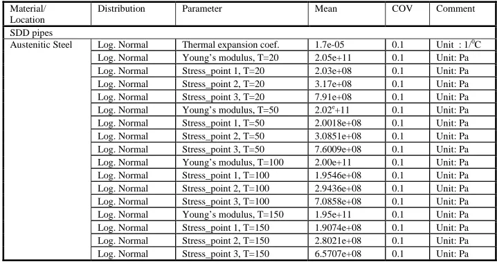
The coefficients of variation for all the random variables were adopted from data and approaches presented in papers listed in (Alzbutas, 2003). In this analysis, the logarithmic-normal distribution was used for mechanical properties and geometry parameters. The peak points of the load curves are as also considered to be random variables with normal distributions. The selected random variables, distributions and coefficients of variation are presented in Tables 1-3.

Table 1. The material properties and parameters expressed as random variables

Material/ Location

Distribution Parameter Mean COV Comment

SDD pipes

Log. Normal Thermal expansion coef. 1.7e-05 0.1 Unit : 1/0 C Log. Normal Young’s modulus, T=20 2.05e+11 0.1 Unit: Pa Log. Normal Stress_point 1, T=20 2.03e+08 0.1 Unit: Pa Log. Normal Stress_point 2, T=20 3.17e+08 0.1 Unit: Pa Log. Normal Stress_point 3, T=20 7.91e+08 0.1 Unit: Pa Log. Normal Young’s modulus, T=50 2.02e

+11 0.1 Unit: Pa Log. Normal Stress_point 1, T=50 2.0018e+08 0.1 Unit: Pa Log. Normal Stress_point 2, T=50 3.0851e+08 0.1 Unit: Pa Log. Normal Stress_point 3, T=50 7.6009e+08 0.1 Unit: Pa Log. Normal Young’s modulus, T=100 2.00e+11 0.1 Unit: Pa Log. Normal Stress_point 1, T=100 1.9546e+08 0.1 Unit: Pa Log. Normal Stress_point 2, T=100 2.9436e+08 0.1 Unit: Pa Log. Normal Stress_point 3, T=100 7.0858e+08 0.1 Unit: Pa Log. Normal Young’s modulus, T=150 1.95e+11 0.1 Unit: Pa Log. Normal Stress_point 1, T=150 1.9074e+08 0.1 Unit: Pa Log. Normal Stress_point 2, T=150 2.8021e+08 0.1 Unit: Pa Austenitic Steel

Log. Normal Stress_point 3, T=150 6.5707e+08 0.1 Unit: Pa

Table 2. The geometry parameters of random variable

Material/ Location

SDD Pipes

Austenitic Steel Log. Normal Wall thickness 0.003 0.05 Unit: m

Table 3. The peak points of load curve parameters expressed as random variables

Normal LoadUnit 1, pressure in SDD header -33840 0.1 Unit: Pa Normal LoadUnit 2, pressure in SDD header 33840 0.1 Unit: Pa Normal LoadUnit 3, pressure in vertical vent pipe -33740 0.1 Unit: Pa Normal LoadUnit 4, pressure in vertical vent pipe 33740 0.1 Unit: Pa Normal LoadUnit 5, pressure in vertical vent pipe -33740 0.1 Unit: Pa Normal LoadUnit 6, pressure in vertical vent pipe 33740 0.1 Unit: Pa Normal LoadUnit 8, force on the end vertical vent pipes 40.43 0.1 Unit: N Normal LoadUnit 10, force from pool swelling on SDH 752.50 0.1 Unit: N Normal LoadUnit 11, temperature in SDD header 90.0 0.1 Unit: 0

C Normal LoadUnit 12, temperature in vertical vent pipe 98.96 0.1 Unit: 0

C

4.2 Selected Limit States for analysis

The steam distribution devices with the vertical vent pipes, which are inserted under the water of condensing pools, connect the dry well and the wet well. These components should be capable of withstanding the dynamic loads from pressure surges during an accident. A deterministic structural integrity analysis was previously performed. The aim of the structural integrity analysis of the SDD subjected to a maximum design basis accident (MDBA) was to evaluate the following:

1. Structural integrity of the SDD header;

2. Structural integrity of the connection between the SDD header and the vertical vent pipes.

(6)

1. Limit State 1 – Response of Element 311 (Fig. 4a; first integration point). The limit state is defined as follows: Stress Equivalent > 4.61e+8 Pa. This element is on the SDH adjacent to the connection of the SDD header and the vertical vent pipe. When this limit state inequality is true, the strength limit in the SDD element is reached and the SDD header and the vertical vent pipe connection are assumed to fail. The value 4.61e+8 Pa is the austenitic steel (12X18H10T – steel of SDD pipelines) ultimate strength at temperature 100 0C.

2. Limit State 2 – Response of Element 16 (Fig. 4b; first integration point). The limit state is defined as follows: Stress Equivalent > 4.61e+8 Pa. This element is the SDH pipe element adjacent to the SDD header support constrains. When this limit state inequality is true, the strength limit in the SDD element is reached and the SDD header at the SDD header support is assumed to fail.

4.3 Probabilistic Analysis Results using RS/MCS Method

The RS/MCS method was used to determine a probability function for probabilistic failure analysis of the steam distribution headers and their connections with the vertical vent pipes.

The RS method was used to determine response surfaces (dependence functions) for the two limit functions in terms of the random variables. The number of simulations was 60. The following dependence function was determined for the respective limit states:

1. Limit State 1 - Element Response (311 is the element number (first integration point) – Fig. 3a) Stress Equivalent > 4.61e+8.

Y1=-13875580.8014+603.4843*L1-10.7625*L2-1712.1794*L3-617.2748*L4+102.1057*L5

+241.5262*L6-120555.6553*L8+17776.9545*L10+11085.6583*L11+713550.8232*L12-7016494979.2115*T1+4632751991553. 4200*Te1-0.0003*Yt1+0.0993*St1t1+0.0644*St2t1

+0.0182*St3t1+0.0010*Yt2-0.1095*St1t2-0.5546*St2t2-0.0109*St3t2-0.0012*Yt3-0.2480*St1t3

+0.6252*St2t3+0.1797*St3t3+0.0003*Yt4+ 0.1060*St1t4-0.5451*St2t4+0.2293*St3t4 (1)

2. Limit State 2 - Element Response (16 is the element number (first integration point) – Fig. 3b) Stress Equivalent > 4.61e+8.

Y2=102061872.8991-6722.2946*L1-5926.9834*L2 + 472.0384*L3-92.0005*L4 +66.9088*L5 +881.5703*L6+55636.7556*L8

+161550.6962*L10 +26454.5521*L11+362417.5910*L12-30985487615.4400*T1+533274230270.3110*Te1

+0.0000*Yt1-0.9411*St1t1-0.0236*St2t1 +0.2083*St3t1 -0.0002*Yt2 +0.5818*St1t2

+0.2210*St2t2-0.1451*St3t2+0.0005*Yt3-0.1878*St1t3-0.0428*St2t3-0.0592*St3t3 +0.0001*Yt4-0.0837*St1t4 -0.0614*St2t4

+0.1013*St3t4 (2)

where the response variable y is used in limit state 1 and 2, i.e. y > 4.61e+8; L1 - LoadUnit 1, maximum pressure point in SDD header; L2 - LoadUnit 2, maximum pressure point in SDD header; L3 - LoadUnit 3, maximum pressure point in vertical vent pipe; L4- LoadUnit 4, maximum pressure point in vertical vent pipe; L5 - LoadUnit 5, maximum pressure point in vertical vent pipe; L6 - LoadUnit 6, maximum pressure point in vertical vent pipe; L8 - LoadUnit 8, maximum force point on the end of vertical vent pipe; L10 - LoadUnit 10, maximum force point from pool swelling on SDH; L11 - LoadUnit 11, maximum temperature point in SDD header; L12 - LoadUnit 12, maximum temperature point in vertical vent pipe; T1 - wall thickness of the SDD pipes; Te1 - thermal expansion coefficient of austenitic steel; Yt1 - Young’s modulus at temperature T=20; St1t1 – stress point 1 at T=20; St2t1 – stress point 2 at T=20; St3t1 – stress point 3 at T=20; Yt2 - Young’s modulus at temperature T=50; St1t2 – stress point 1 at T=50; St2t2 – stress point 2 at T=50; St3t2 – stress point 3 at T=50; Yt3 - Young’s modulus at temperature T=100; St1t3 – stress point 1 at T=100; St2t3 – stress point 2 at T=100; St3t3 – stress point 3 at T=100; Yt4 - Young’s modulus at temperature T=150; St1t4 – stress point 1 at T=150; St2t4 – stress point 2 at T=150; St3t4 – stress point 3 at T=150.

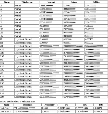
Next, the MCS method was used for probabilistic failure analysis of the steam distribution headers and their connections with the vertical vent pipes. The equations obtained using RS/MCS were used as internal response functions in the MCS analysis. The number of MCS simulations was 1,000,000. The nominal values of material properties and geometry parameters and normal distribution (10%) of loading was used in this analysis. Using this method of probabilistic analysis the probabilities of the limit states were calculated.

The obtained mean, standard deviation, COV, skewness and kurtosis coefficients for random variables are presented in Table 4.

The probability of failure Pi for i-th limit state as the corresponding safety index (beta βi) is presented in Table

(7)

Table 4. The data of Random Variables

Name Distribution Nominal Mean Std.Dev.

L1 Normal -33840.000000 -33840.000000 3384.000000

L2 Normal 33840.000000 33840.000000 3384.000000

L3 Normal -33740.000000 -33740.000000 3374.000000

L4 Normal 33740.000000 33740.000000 3374.000000

L5 Normal -33740.000000 -33740.000000 3374.000000

L6 Normal 33740.000000 33740.000000 3374.000000

L8 Normal 40.430000 40.430000 4.043000

L10 Normal 752.500000 752.500000 75.250000

L11 Normal 90.000000 90.000000 9.000000

L12 Normal 98.960000 98.960000 9.896000

T1 Logarithmic Normal 0.003000 0.003000 0.000150

Te1 Logarithmic Normal 0.000017 0.000017 0.000002

Yt1 Logarithmic Normal 205000000000.000000 205000000000.000000 20500000000.000000

St1t1 Logarithmic Normal 203000000.000000 203000000.000000 20300000.000000

Table 5. Results related to each Limit State

Name Definition Probability 5% 95% Beta

Limit State 1 Y1 > 461000000.000000 7e-006 3.61345e-006 1.03865e-005 -4.34379

Limit State 2 Y2 > 461000000.000000 6.2e-005 5.19216e-005 7.20784e-005 -3.83815

The calculated probability of the ‘Limit state 1’ is 7e-6. This indicates that the strength limit in SDD header pipe element was reached with a probability of 7e-6 at nominal loading points and the SDD header and vertical vent pipe connection could fail with a probability of 7e-6.

The calculated probability of the ‘Limit state 2’ is 6.2e-5. This indicates that the strength limit in SDD element was reached with a probability of 6.2e-5 at nominal loading points and the SDD header near the SDD header support constrains could fail with a probability of 6.2e-5.

The probability function (1) was used for determination of the relation between the probability of ‘Limit state 1’ and the applied loads, i.e. pressure, forces and temperatures. The results of the probabilistic analysis are presented in Fig. 4 and Fig. 5.

(8)

The failure probabilities of the SDD header and vertical vent pipe connection (SDH pipe element adjacent to vertical vent pipe) due to force on the end vertical vent pipe occurs at a force approximately equal to 0.04 kN, and the failure probabilities of the SDD header and vertical vent pipe connection occurs with a probability of 1 at a force approximately equal to 3.5 kN (Fig. 4, b). The maximum force obtained in the thermo hydraulic analysis is approximately equal to 0.0404 kN.

The influence of the force from swelling for failure of the SDD header and vertical vent pipe connection (SDH pipe element adjacent to vertical vent pipe) is small. Therefore the failure probabilities of the SDD header and vertical vent pipe connection due to force from swelling were not presented.

The failure probabilities of the SDD header and vertical vent pipe connection (SDH pipe element adjacent to vertical vent pipe) due to the resultant temperature in the SDD header and vertical vent pipe occurs at a resultant temperature of approximately equal to 85 0C. The maximum temperature for the MDBA turns out to be approximately 120 0C therefore the failure probabilities for the temperature was carried out up to 150 0C. The failure of the SDD header and vertical vent pipe connection occurs with a probability of 0.00235 at the resultant temperature of 150 0C (Fig. 5, a). The maximum temperature obtained in the thermo-hydraulic MDBA simulation is approximately equal to 120 0C. The probability function (2) was used for determination of the relation between probability of the ‘Limit state 2’ and the force from swelling. The influences of the pressure, of the force on the end vertical vent pipe and of the temperature for failure of the SDD header near to the SDD header support constrains are small. Therefore the failure probabilities of the SDD header near to the SDD header support constrains due to these loads were not presented.

0 0.2 0.4 0.6 0.8 1

0 0.1 0.2 0.3 0.4 0.5 0.6 0.7 0.8 0.9 1 Pressure, MPa

Pr

obability

0 0.2 0.4 0.6 0.8 1

0 0.5 1 1.5 2 2.5 3 3.5

Force on the end vertical vent pipe, kN

Pro

b

ab

ility

a) b)

Fig. 4

.

Failure probabilities of the SDD header and vertical vent pipe connection (SDH pipe

element adjacent to vertical vent pipe) due to the resultant pressure in the SDD header

and vertical vent pipe (a) and to the force on the end of the vertical vent pipe (b)

Failure probabilities of the SDD header near the SDD header support constrains due to the force from swelling of the SDD header occur at a force approximately equal to 0.7 kN, and failure probabilities of the SDD header near the SDD header support constrains occurs at the probability of 1 at a force approximately equal to 3.2 kN (Fig. 5, b). The maximum force obtained in the thermo-hydraulic model is approximately equal to 0.752 kN.

0 0.0005 0.001 0.0015 0.002 0.0025

0 20 40 60 80 100 120 140

Temperature, C

Pro

b

ab

ility

0 0.2 0.4 0.6 0.8 1

0 0.5 1 1.5 2 2.5 3 3

Force from swelling on the SDD header, kN

P

roba

bility

.5

a) b)

(9)

5. SUMMARY AND CONCLUSIONS

The probabilistic failure analysis of a representative steam distribution header and its connections to the vertical vent pipes during a MDBA was carried out. The Monte Carlo Simulation and Response Surface methods were used for probabilistic analysis.

The results of the probabilistic analysis of failure of the steam distribution headers and their connections with the vertical vent pipes show that:

• The strength limit in the SDD header pipe element would be reached and the SDD header and vertical vent pipe connection would fail with a probability of 7e-6;

• The strength limit in the SDD header pipe element would be reached and the SDD header near to the SDD header support constrains could fail with a probability of 6.2e-6.

According to the results of the analysis the probability of failure of the steam distribution header pipes is small in case of the maximum design basis accident.

ACKNOWLEDGMENTS

This work was supported by the U.S. Department of Energy, National Nuclear Security Administration. The authors also want to extend thanks to the administration and technical staff at the Ignalina NPP, for providing information regarding operational procedures and operational data.

The U.S. Government makes no endorsement of the results of this work.

REFERENCES

ProFES: Probabilistic Finite Element System, Applied Research Associates, Inc., Southeast Division, 8540 Center Dr., Suite 301 Raleigh, NC 27615, USA.

Kulak R.F. and Fiala C., (1988), Jrnl. of Nuclear Engineering and Design, Vol. 106, pp. 47-68.

Kulak, Ronald. F. and Marchertas, Paul. V., (2003), Transactions 17th International Conference on Structural Mechanics in Reactor Technology (SMiRT17), B01-2.

Algor Finite Element Analysis System, ALGOR Instruction Manuals. Algor, Inc. Pittsburgh, 2000.

Belytschko T., Lin J.I., and Tsay C.S., (1984), Jrnl. of Computer Methods in Applied Mechanics and Engineering, Vol. 42, pp. 225-251

Mark A. Cesare and Robert H. Sues, (1999), American Institute of Aeronautics and Astronautics, AIAA 99-1607, pp. 1-11.

COCOSYS V1.2 Program Reference Manual, GRS mbH, 2001.