Estimation of Effects of Quantitative Trait Loci in Large Complex Pedigrees

(1)

Estimation of Effects of Quantitative

Trait

Loci

in

Large

Complex Pedigrees

T.

H.

E. Meuwissen

and

M. E.

Goddard"

Institute for Animal Science and Health, 8200 AB Lelystad, Netherlands and *Animal Genetics and Breeding Unit, University of New England, Armidale, NSW 2351, Australia

Manuscript received May 17, 1996 Accepted for publication January 13, 1997

ABSTRACT

A method was derived to estimate effects of quantitative trait loci (QTL) using incomplete genotype information in large outbreeding populations with complex pedigrees. The method accounts for background genes by estimating polygenic effects. The basic equations used are very similar to the usual linear mixed model equations for polygenic models, and segregation analysis was used to estimate the probabilities of the QTL genotypes for each animal. Method R was used to estimate the polygenic heritability simultaneously with the QTL effects. Also, initial allele frequencies were estimated. The method was tested in a simulated data set of 10,000 animals evenly distributed over 10 generations, where 0, 400 or 10,000 animals were genotyped for a candidate gene. In the absence of selection, the bias of the QTL estimates was <2%. Selection biased the estimate of the Aa genotype slightly, when zero animals were genotyped. Estimates of the polygenic heritability were 0.251 and 0.257, in absence and presence of selection, respectively, while the simulated value was 0.25. Although not tested in this study, marker information could be accommodated by adjusting the transmission probabilities of the genotypes from parent to offspring according to the marker information. This renders a QTL mapping study in large multi-generation pedigrees possible.

.~

I

N molecular biology two approaches are used to de- tect quantitative trait loci (QTL): (1) the candidate gene approach (e.g., ROTHSCHILD et al. 1994) and (2)

linkage to molecular markers (e.g., ANDERSSON et al.

1994). With both approaches, the information on the genotypes at the QTL is likely to be incomplete, because of nongenotyped animals and, in the case of molecular markers, due to recombination between markers and QTL. Exclusion of many nongenotyped animals from the data analysis results in poor estimates of correction factors (e.g., herds, seasons) and poor correction for the effects of selection, which may be strong in livestock populations (HENDERSON 1984). Furthermore, the nongenotyped animals will provide information on the effects of the QTL: segregation analysis can estimate QTL effects without any animal being genotyped (ELSTON and STEWART 1971).

Methods for the detection of QTL by markers have been suggested in outbreeding populations with a fixed family structure, mostly paternal half sib families (HA-

LEY et UL. 1994; KNOTT et al. 1994)

.

The accuracy of the estimate of QTL effects and of their site increases substantially when more generations with possible re- combinations are included in the analysis ( DARVASI and SOLLER 1995)

.

This requires estimation of QTL effects in large and complex pedigree structures. Segregation analysis methods (ELSTON and STEWART 1971; HAS STEDT 1991; FERNANDO et al. 1993; STRICKER et al. 1995)

Cmrespondingauthm: T. H. E. Meuwissen, DLO, Institute f o r h i m a l Science and Health, Box 65, 8200 AB Lelystad, The Netherlands. E-mail: [email protected]

Genetics 146 409-416 (May, 1997)

are computationally very demanding in large complex pedigrees with many loops, many unknown parameters,

e.g., many herd effects, and with polygenic effects (the

combined effect of many small background genes). Monte Carlo Markov chain (MCMC) methods have been proposed for large complex pedigrees while ac- counting for polygenic effects ( GUO and THOMPSON 1992), but they are computationally very demanding and the Markov chain may get stuck in a subset of the sampling space, which hampers routine usage. For the near future it is expected that many outbreeding populations and species will have markers and candidate genes genotyped for many characteristics and thus a data analysis for QTL effects will become a standard routine, which calls for less computer-intensive and problem-free methods.

Mixed models have become widely used in animal breeding to estimate polygenic breeding values of animals (random effect) in large complex data structures while correcting for various fixed effects (e.g., herds, seasons) ( HENDERSON 1984). The aim of the present study is to include the estimation of QTL effects in a mixed model that also accounts for the effects of polygenes and various fixed effects. The approach is similar to that of HOFER and KENNEDY ( 1993) and the differences between the present and their method are described in DISCUSSION. The inclusion of the estimation

(2)

410 T. H . E. Meuwissen and M. E. Goddard

MATERIALS AND METHODS

The model: The general model for the data is y = X b + Z u + Z Q q + e ,

where y = ( n* 1 ) vector of data; b =

( p *

1 ) unknown vector of fixed effects ( e . g . , herds) ; u = ( t* 1 ) unknown vector of polygenic effects (random; t = number of animals) ; q = ( 3

*

1 ) unknown vector of effects of the QTL genotypes (in the case of three genotypes) ; e =

( n* 1 ) unknown vector of environmental effects; X =

( n * p ) known incidence matrix linking fixed effects to records; Z = ( n * t) known incidence matrix linking animals to records; Q = ( t* 3 ) unknown incidence matrix with a one at position (

j ,

k ) if animal j has genotype

k and zeros elsewhere. The variance of the polygenic effects, u , is G = Aa

f

,

where A = the matrix of relation- ships between the animals (HENDERSON 1984), and Var ( e ) = R = Ia?. Extension to more general R is straightforward, but R is assumed diagonal. Further, define V = Var ( y ) = ZGZ

'

+

R .

Estimation of QTL and polygenic effects: The log-

likelihood of the data is

In L ( y l q , b ) = const

+

In C p ( Q ) exp[-% { Q

X ( y - ZQq - Xb)'V"(y - ZQq -

= ) I

, ( 1 )

where const is the constant that does not depend on q , b , and u ,

2,

denotes summation over all possible matrices Q , i.e., all possible combinations of genotypes, and

p

( Q ) is the prior probability of the QTL genotypes as described by Q . If animals are unrelated and V is diagonal, the term exp [ - 1/2(y - ZQq - X b ) 'V-' ( y -

ZQq

-

Xb ) ] can be written as the product of individual likelihoods:

n,

exp [ -1/2(yi - ZiQq - X;b)'/Vii)],

where Zi and X, denote the ith row of Z and X , respectively, and Vii = the ith diagonal element of V . In this case, the contribution of animal i does not depend on that of the other animals, and likelihood (1 ) can be computed by segregation analysis algorithms (e.g., ELS TON and STEWART 1971; or FERNANDO et al. 1993 for large data sets). Because the e effects are independent, rewriting likelihood (1) in terms of 6 will render the contributions of every animal as independent as possible, where superscript denotes the estimate of the effects. Let C = ( Z

'

R"Z

+

G-') - I and because V" = R" -

R"ZCZ'R", likelihood ( 1 ) can be written as

I

In L ( y [ q , b ) = const

+

In

C p ( Q )

{ Q

X exp[-'b2G'(R - ZCZ')-'G

1

where 6 = RV p 1 ( y - ZQq - Xb ) (from regression

theory), and u : is the sth diagonal element of the matrix R - ZCZ '. The approximation in ( 2 ) holds when the off-diagonals of R - ZCZ

' are small and is exact if

the animals are unrelated.

The derivative of In L ( y

1

q , b ) with respect to q k is

In L ( y l q , b)/6qk = L ( y l q , b ) "

x

{

c ~ ( Q )

c

n

exp[-1~2;:/a:1

Q .s, I

I

X

6

- % e ^ : / U : / S q k = L ( y l q , b ) "

,

x {

@ R ( i , k )

C

p ( Q )

n

5 exp[-%e^?/a?l

1 x

6

- %z:/af/6qk= Xwk6 - % e ^ : / f f : / b q k , ( 3 )

2

where denotes summation over all records i of animals that have genotype k denoted by Q , and X C C k K ( L , k )

denotes summation over all possible matrices Q where record i was produced by an animal with genotype k ;

65; / 6 q k is assumed zero for animals that do not have genotype k , and

w k = L ( y l q , b ) -

I {

p ( Q )

n e x p [ - ' h ~ P / o ? l ,

@ R ( i , k )

1

which is the probability that animal

j ,

which produced record i, has genotype k given G .

The values of

wzk

can be calculated by segregation analysis algorithms, e.g., ELSTON and STEWART ( 1971 ) ,

FERNANDO et al. (1993). These algorithms require the probability that animal

j

has phenotype 6, conditional on having genotype k , for all genotypes k , which is

~ ( j l k )

n,

e x p [ - ' h z f / a ~ I ,

where the product is over the records i of animal

j .

If animal j does not have a record, P (

j l

k ) = 1, for all k .

And if animaljis known to have genotype k , for instance from a DNA analysis, P ( j l k ) = 1 and P ( j l k ' ) = 0, for

k' # k . The segregation analysis algorithm of KERR and

KINGHORN ( 1996) will be used because it can approximate genotype probabilities, w ' k , in large pedigrees

with loops [by making iterative use of the algorithm of FERNANDO et al. ( 1993) ] .

The value of tr conditional on genotype k is

zt

= ( y j - ijk - C ] ( k ) -

Yb)

*

( 1 - h') (yj - q k - x j b ) ,

where Gj( k ) = estimated polygenic effect of animal

j

that produced record i conditional on having genotype

(3)

x

( 1 - h 2 ) / O f = ( y i - (ik - 6 j ( k ) -

xb)/OP,

because a f =

CT:

-

(a;

+

n i 2 ) - l = ( 1 - h')03 for unrelated animals. This assumption of unrelated animals may seem rather crude, but a similar cancelation occurs when the offdiagonals of ( R - ZCZ

'

) are not ignored, which is possible for known Q and results also in the division by

0 3 .

Equating formula ( 3 ) to zero yields an estimating equation for q k :

Estimation of b and u follows from similar derivations (see APPENDIX ) and the equations can be combined to yield the mixed model equations:

D W'X 0

X ' W X ' X

z'w z'x z'z

+

A-'A X'Z

][!I

=

[

-

[

i]

> ( 4 )

where A =

0 3 / 0 2 , ,

W = ( n * 3 ) matrix of elements

Kk,

0 0

1

and r is ( 3 * 1 ) vector with element k : rk =

C j

w k G j ( k ) ,

with j being the animal that produced record i. Equa- tions 4 are very similar to the ordinary mixed model equations (HENDERSON 1984) that would result if each record y i was replicated three times, where each repli- cate obtains a weight of

w,k

(for k = 1, 2, and 3 ) ( see also JANSEN, 1992). The difference being that the r

vector in Equations 4 replaces the usual W'ZQ term in the ordinary mixed model equations.

It may be noted that Q in Equation 4 is the average estimate of the polygenic effects, where averaging is over the three genotypes weighted by the genotype probabilities. For the estimation of r and W, Gj( k ) is needed,

i.e., the estimate of the polygenic effect conditional on animal j having genotype k . The values of GI( k ) are a p proximated by assuming that the conditioning on genotype k hardly affects the expectation of u i , of the other animals j ' ( j ' # j )

.

Then, using Equations 4,

6 j ( k ) = 6,

+

q ( w i q -

qk)/(z'z

+

A"k) ( 5 )

where ( Z

'

Z

+

A"A) j I denotes the ( j , j ) diagonal ele-

ment of the matrix Z

'

Z

+

A"A, and

4

= the number of records that animal j produced.

Because estimation of, for instance, W depends on estimates for

q ,

whose estimation involves W again, iteration is needed to solve for all the effects. The segregation analysis algorithm requires prior frequencies,

p,,,,

of one of the two QTL alleles (the other one is ( 1 -

p,)

) , which are updated in Step 2 of the iteration scheme if

p,

is unknown. The iteration scheme that is used here is as follows:

Step 1. Update W and D using the current estimates of q , b , Q , p,,,, and the iterative algorithm of

KERR

and KINGHORN ( 1996). Only one iteration of this algorithm is performed to save computer time. Step 2. If prior allele frequencies of the QTL are un-

known, they are updated by

jPr

= &&rp(

l4$

+

'/?w2)

/

nbase = number of base animals (animals with no parents in pedigree) , and summation is over the base animals.

Step 3. Solve for b and Q using the current estimates of Wq in Equation 4. Calculate also

Q(k)

for all genotypes k using Equation 5 and calculate r .

Step 4. Solve for q in Equation 4, using current estimates of D , W , r , b and Q . If the subsequent estimates q have converged, stop; otherwise go to step 1.

Estimation of polygenic heritability: Estimation of the polygenic heritability, h 2 , is difficult in situations with little information on the genotypes, because the pattern of covariances between relatives due to the QTL effects is similar to those due to the polygenic effects. The likelihood surface will be very flat, which means that the approximation of the likelihood in Equation 2 needs to be very good to estimate the polygenic h 2 .

Otherwise, a biased h2 will be found.

Heritability estimation by method R (REVERTER et al.

1994) avoids calculation of the likelihood or its derivatives and is thus useful in data sets that are too large for direct calculation of the likelihood, as is the case here. Let

G,

be the estimate of the polygenic effects from Equation 4 when at random 50% of the data are discarded, then the regression of u on Q,r, R = Q' A ~ ' G y / Q ~ A ~ ' Q y , is on average 1 if the correct heritability is used. This is because the expected change of BLUP (best linear unbiased prediction) estimates is zero as more information becomes available. If E ( R )

<

1, the heritability used to calculate

G

and Q, was too high and vice versa.

The algorithm that was used is as follows:

Step 0. Start with a (good) guess of the heritability h'

and set h: = h: = h 2 , where h;- and h't, are lower and upper bounds for the heritability, respectively. Step I . Estimate Q using the current heritability h' from

Equation 4.

(4)

412 T. H. E. Meuwissen and M. E. Goddard

Step 3. Estimate i i X i and R, for every subsample i = 1,

. . .

, 50. Let NR<, be the number of R,

<

1. If

>

32, heritability needs to be decreased: go to Step 4a. If NH<l

<

18, heritability needs to be increased, go to Step 4b. Otherwise, 18 5 NK<I 5 32, which

is approximately a 95% confidence interval for a binomial variable with 50 samples and 50% success rate. Hence, Prob ( R , .

<

1 ) is not significantly differ-

ent from SO%, which is the probability at the true heritability value. Thus, h2 is found and iteration is stopped.

Step 4a. If h' = h2, decrease h' and h;, by

lo%,

otherwise set h$ = h' and then h' =

y2

(h:,

+

h;)

.

Go to Step 1.

Step 4b. If h' = h$, increase h2 and h$ by

lo%,

otherwise set h:, = h' and then h' =

y2

(h:,

+

h:)

.

Go to Step 1.

Computer time can be saved by generating fewer subsamples (adjusting the 95% confidence interval accord- ingly) and, after the algorithm stops, restarting it with a larger number of subsamples.

Simulation: To test whether the previously described method can estimate QTL effects, a simulation study was conducted. Fifty data sets were simulated of 10,000 animals each, which came from 10 discrete generations. Each generation consisted of 1000 animals that were the offspring of 50 sires that were mated to five dams each, except for generation 1 that consisted of unrelated base animals. The sires and dams were either selected on phenotype or randomly selected. The QTL genotypes, AI Al

,

A1 A', and AQAP, of the base animals were sampled at random with probabilities:

p$l,

2p,,(

1

-

p,)

,

and ( 1 -

p,)

'

, where

p,

was 0.5 and 0.1, respec-

tively, with random and with phenotypic selection. An initial frequency of 0.1 was used in the situation with phenotypic selection, because, if an initial frequency of 0.5 was used, the positive allele reached fixation around generation 5 and the last five generations of the simulation would not contribute anymore. The genotypes of the animals of later generations were sampled according to the Mendelian segregation probabilities. In the base population, the effects of the polygenes were sampled from N(0, 0.25), i.e., 02, = 0.25, and in later

generations u, was sampled from N ( u,

+

u d ) ;

'/'a:) , where u, ( u d ) denotes the polygenic effect of the sire (dam) of animal i. The effect of inbreeding on the within family variance was neglected because the effective population size was quite large ( 4 * 50* 250,'

( 50

+

250) = 166 animals per generation)

.

In situations where inbreeding is important, its effect is easily included in the additive relationship matrix A (HEN- DERSON, 1984). All animals had records from

yz = q ( genotype of i )

+

u,

+

e , ,

where e, was sampled from N ( 0 , 0.75), i.e., a: = 0.75;

q ( A I A 1 ) = 1; q ( A , A , ) = 0; and q(A2A2) = -1. Hence,

no fixed effects were simulated nor included in the analysis of the data.

The genotypes of 0, 400, or all 10,000 animals were known, when the QTL effects were estimated, i.e., the effect of a candidate gene is estimated. With 400 known genotypes, each generation had at random 40 animals genotyped. The situation with all genotypes unknown is a worst case scenario to test whether the information from the nongenotyped animals yields unbiased information, i.e., whether the approximated genotype probabilities are sufficiently accurate. Also, because the effect of the QTL is large, the records provide a substantial amount of information about the genotype probabilities.

RESULTS

Table 1 shows the results of the parameter estimates in the absence of selection. The variance components

02, and a: were assumed known here, which is approxi-

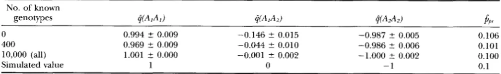
mately the case when the effect of the QTL is small relative to that of the polygenes. This was not the case in these simulations, but otherwise the effects of the QTL could not have been estimated in the case of all genotypes unknown. With 0 or 400 known genotypes, the effects of the AI AI and A2A2 genotypes were slightly underestimated. This bias seems insignificant in view of the size of the effect. When only 400 and zero animals are genotyped, the standard errors of the estimates increased only by -20 and 40%, respectively, relative to the situation with all animals typed, which suggests that the nongenotyped animals provide a significant amount of information. This information probably reduces as the effects of the QTL genotypes are smaller. Estima- tion of the prior frequency of the AI allele was accurate. Table 2 shows the same results with phenotypic selection of the parents. In the absence of genotyped animals, the estimate of the AIA2 genotype was highly underestimated. In the early generations many animals have genotype A2A2, which results in accurate information about q ( A 2 A 2 ) , while in the late generations the frequency of the Al allele was high, which provided accurate information about q ( AIAl )

.

The analysis re- covered information from differences between generation means because no fixed effects (e.g., generation effects) were included in the model. In the intermediate generations where AIAP genotypes were most com- mon, the analysis underestimated the frequency of the

AI allele and hence biased the estimate of the A ~ A Q

genotype effect. With 400 genotyped animals, the bias of

q(

A1A2) has almost disappeared. This selection bias seems to reduce markedly if some genotype information is available.

(5)

TABLE 1

Estimates of QTL effects, q, and prior allele frequency,

&.,

when selection is at random (50 replicated data sets) No. of known

genotypes AIAI AI) & A d z ) q(A2Az) PP

0 0.980 2 0.007 -0.005 ? 0.008 -0.985 ? 0.007 0.500

400 0.975 2 0.006 -0.002 ? 0.006 -0.980 ? 0.007 0.500

10000 (all) 0.997 2 0.005 -0.003 ? 0.005 -1.001 2 0.005 0.500

Simulated value 1 0 -1 0.5

Values are S E .

to the size of the heritability. The estimates of the effects of the QTL were similar to those with known heritability and their standard errors were slightly increased (com- pare to Tables 1 and 2 ) .

DISCUSSION

Properties of the QTL estimation method: A method was derived to estimate the effects of QTL in large data structures with incomplete genotype information, by solving Equations 4. Solving Equations 4 is computationally equivalent to solving the usual mixed model equations, but these equations have to be solved within each iteration because the matrix of weights W depends on the solutions of ( 4 ) . The number of iterations needed was typically -25, which makes the method roughly 25 times slower than the usual mixed model breeding value estimation methods.

In the absence of selection, the presented method yielded virtually unbiased results. With the strong selection that was simulated in Table 2, the estimate of the effect of the intermediate genotype was somewhat biased. In QTL effect estimation experiments, selection will be less strong and a higher proportion of the animals will be genotyped. Also, the method-R estimates of the polygenic heritability seemed unbiased in the absence of selection and showed an insignificant bias when selection was present. The estimates of QTL effects, heritability and genotype probabilities assumed known environmental variance, 0 ; . In practice, the data or similar data have

often been analyzed by a complete polygenic model yielding a REML (residual maximum likelihood) variance component estimate for c;, that is, with the QTL

effect pooled together with the polygenic effects. In the present data sets with random and phenotypic selection, average estimates of a: of 0.742 5 0.0035 and 0.742

-+

0.0016, respectively, were obtained from

the standard computer package VCE (GROENEVEL.D

1994). The simulated value was 0.75.

Simultaneous estimation of polygenic heritability and QTL effects increased the computing time substantially, because it involves many repeated estimations of the QTL effects. However, the variance due to the QTL is often small relative to the polygenic variance and the heritability estimate of a pure polygenic model will be appropriate. The total genetic variance is relatively easy to estimate, but it is difficult to distinguish between QTL and polygenic variance, which implies that a too high estimate of h' will result in underestimates of the QTL effects and vice versa. In the case of a QTL mapping experiment, many estimations of the QTL effects are needed, each with a slightly different map position of the putative QTL, which makes that a single estimate of heritability seems sufficient.

We also derived formulas to estimate the standard error of the estimates of the QTL effects, but these resulted in underestimates because they only approximately accounted for the uncertainty about the genotypes of the animals ( results not shown)

.

However, standard errors can be obtained from replicated Monte Carlo simulations of the data using the estimated QTL effects as the true effects, using the same pedigree structure as in the real data with the same animals being genotyped (genotypes differ and are sampled because they are unknown). The variance of the estimates from the simulated data reflects the error variance of the estimates from the real data. Because estimation of QTL

TABLE 2

Estimates of QTL effects, q, and prior allele frequency, p p , with phenotypic selection (50 replicated data sets) No. of known

genotypes AIAI AI) AIAI AI) #A.Ad _P,Jr

0 0.994 ? 0.009 -0.146 ? 0.015 -0.987 ? 0.005 0.106

1.001 2 0.000 -0.001 ? 0.002 -1.000 2 0.002 0.100

400 10,000 (all)

Simulated value 1 0 -1 0.1

0.969 2 0.009 -0.044 5 0.010 -0.986 5 0.006 0.101

(6)

414 T. H. E. Meuwissen and M. E. Goddard

TABLE 3

Estimates of polygenic heritability, h2, QTL effects, q, and prior d e l e frequency, p p , when no animals

are genotyped (50 replicated data sets)

Selection of parents

at random On phenotype

h' 0.251 5 0.003 0.257 ? 0.002

# A I A I ) 0.976 ? 0.008 0.978 t 0.009

~ ( A I A Z ) -0.011 ? 0.009 -0.137 ? 0.014 ~ ( A Z A Z ) -0.974 ? 0.009 -0.983 ? 0.005

Values are 5SE.

effects is reasonably fast, despite of the iterations involv- ing updating of W , this will not take too much computing time and standard errors may only be needed for promising QTL. Under the usual assumptions of asymp- totic normality of the estimates, these error variances can be used for significance testing. If the Monte Carlo estimates seem nonnormal, the permutation test, which requires analysis of reshuffled data, is a robust method to test whether QTL effects are significant ( CHURCHILL

and DOERGE, 1994).

In the presented simulations, both the model that was used to simulate and to analyze the data contained only one QTL. Real data may comprise the effects of several QTL. When marker information is available, the effects of the other QTL may be accounted for by fitting marker effects for them (JANSEN 1994; ZENG 1994). With the candidate gene approach, the information

from the ungenotyped animals may be biased by a sec- ond QTL that affects the genotype probabilities. This bias can be avoided by estimating genotype probabilities without using the data, i e . , using only the known genotypes, following KINGHORN and

KERR

( 1995 )

.

This may increase the standard error of estimates of the QTL effects substantially, but a check whether these estimates are not very different from the ones where data are used to help estimate the genotype probabilities is reassuring.

Alternative methods: In the large data sets that are needed to estimate QTL effects in outbreeding populations, Gibbs sampling methods ( GUO and THOMPSON 1992) provide the only alternative to the methods presented here. Segregation analysis based methods ( e . g . ,

HASSTEDT 1991; FERNANDO et al. 1993) maximize the likelihood directly and computations will soon become prohibitive when there are many loops in the data and the number of parameters for which the likelihood function needs to be maximized becomes large as is usually the case in large data sets ( e . g . , many herds involved). Gibbs sampling methods may get stuck in a part of the parameter space, which requires careful examination of the Gibbs chains, and are very computer intensive. This prevents a quick evaluation of the effect of a marker or a candidate gene in a data set.

The presented method has similarities with the method of KINGHORN et al. ( 1993) in that both methods iterate between a set of mixed model equations and a segregation analysis to update genotype probabilities. The difference is that KINGHORN et al. regressed directly on the genotype probabilities while here the genotype probabilities act as weights for the replicated records (see MATERIALS AND METHODS section Equations 4 ) . The direct regression on the genotype probabilities does not fully account for the uncertainty about an animal having a particular genotype, which was partly accounted for by a correction of components in the mixed model equations. If an animal has genotypes 1 and 2 with probabilities 0.5 and 0.5, respectively, its record, y i , is assumed distributed as N ( 1/2q1

+

0') by direct regression, while in the present method

y L is distributed as N ( ql; u ' ) with probability (weight)

1/2, and N (

*;

0') with probability (weight) (ignor-

ing other fixed and random effects). KINGHORN et al. ( 1993) found biased genotype estimates for which they proposed a correction method that was satisfactory in some situations but not in others.

The present approach is similar to that of HOFER and

KENNEDY (1993). The differences are in the way the summations over all possible combinations of genotypes are approximated. When calculating genotype probabilities, the method of HOFER and KENNEDY uses

exp ( -

v2

Zt

/

a: ) as probability that animal i has EL con-

ditional on having genotype k , while the present method uses exp ( -

v2

Zt

/

a:) , where u is the predic-

tion error variance of t i . The former neglects the effect of the genotype of the animal on the probability density of its polygenic breeding value, i e . , the probability density of the polygenic breeding value is assumed constant across all genotypes. Further, HOFER and KENNEDY as- sume that animals are independent, A = I , when calculating the D matrix in Equation 4. Here, it was assumed that the genotype probability of animals i and j having genotypes r and s, respectively, equals the probability of animal i having genotype r times that of animal ,j

having genotype s that results in D being diagonal, i.e.,

the dependencies between the genotype probabilities are neglected. The last difference between the methods is that HOFER and KENNEDY approximate the expectation EQ( Q' Z h )

=

W'ZQ in the equations for the QTL effects in ( 4 ) , while here this expectation was approximated by r with r, =

xz

Wzkzl1( k ) (see Equation 4 ) ,

which accounts for the effect of animal i having genotype k on its estimate for the polygenic effect. These improvements of the approximations made the estimates of the present method approximately unbiased

(Table 1 ) while that of HOFER and KENNEDY were up

to 14% biased in unselected populations.

(7)

the transmission probability of the genotypes from parents to offspring will deviate from the Mendelian probabilities. For instance, let a sire have haplotypes MI AI

/

M2A2, where MI ( M2) denotes marker alleles and AI

( A 2 ) QTL alleles and MIAl ( M2A2) is the paternally (maternally) inherited haplotype. An offspring that in- herits marker Ml of this sire will have inherited QTL allele AI with probability ( 1 - r ) and A2 with probability

r , where r is the recombination rate between M and

A . This example shows that paternally and maternally

inherited QTL alleles need to be distinguished, which leads to four genotypes: A I / A l , A l

/

A2, AP

/

A I , and A2

/

A2. The genotype probabilities of these four genotypes are calculated by the segregation analysis algorithm using the genotype transmission probabilities that follow from the marker information.

Equations 4 are a simple extension of the usual mixed model equations that are used to estimate polygenic breeding values of animals. The total breeding value of

animal j with record i is EBT/; = dl

+

W!

$.

In the case where Wi and q are estimated with the aid of markers, selection for E B y will constitute a marker assisted selection scheme. FERNANDO and GROSSMAN (1989) suggested a method for the estimation of E B Y , where QTL effects were assumed random with each base animal taken as carrying two unique QTL alleles. In cases with few real QTL alleles, this leads to a very nonnormal distribution of estimated QTL effects, which results in biased EBV estimates. But, assuming that there are two QTL alleles while there are in fact three or four will probably also bias EBV estimates. Research is needed to investigate the effect of the assumed number of QTL alleles on the bias and accuracy of the EBV.

In conclusion, a method was presented that can estimate QTL effects in large pedigrees of any complexity with incomplete genotype or marker information, which will be useful for the screening of candidate genes and marker maps for QTL, and for breeding value estimation in marker-assisted selection schemes.

LITERATURE CITED

~ D E R S S O N , L., C. S. HALEY, H. ELLEGREN, S. A. W o n , M. JOHANS

SON et al., 1994 Genetic mapping of quantitative trait loci for growth and fatness in pigs. Science 263: 1771-1774.

CHURCHILL, G. A,, and R. W. DOERGE, 1994 Empirical threshold Val- ues for quantitative trait mapping. Genetics 138: 963-971.

DARVASI, A,, and M. SOLLER, 1995 Advanced intercross lines, an experimental population for fine genetic mapping. Genetics 141:

1199-1207.

ELSTON, R. C., and J. STEWART, 1971 A general model for the analysis of pedigree data. Hum. Hered. 21: 523-542.

FERNANDO, R. L., and M. GROSSMAN, 1989 Marker assisted selection using best linear unbiased prediction. Gen. Sel. Evol. 21: 467- 477.

FERNANDO, R. L., C. STRICKER and R. C. ELSTON, 1993 An efficient algorithm to compute the posterior genotypic distribution for every member of a pedigree without loops. Theor. Appl. Genet.

87: 89-93.

GROENEWLD, E., 1994 VCE-A multivariate multimode1 REML ( c o ) variance component estimation package. 5th World Congr. Genet. Appl. Livest. Prod. 22: 47-50.

Guo, S. W., and E. A. THOMPSON, 1992 A monte carlo method for combined segregation and linkage analysis. Am. J. Hum. Genet.

51: 1111-1126.

HALEY, C. S., S. A. KNOTT and J.-M. ELSEN, 1994 Mapping quantitative trait loci in crosses between outbred lines using least squares. Genetics 136: 1195-1207.

HASSTEDT, J. S., 1991 A variance components/major locus likelihood approximation on quantitative data. Genet. Epidemiol. 8:

HENDERSON, C. R., 1984 Applications of Linear Models in Animal Breed- ing. University of Guelph, Canada.

HOFER, A,, and B. W. KENNEDY, 1993 Genetic evaluation for a quantitative trait controlled by polygenes and a major locus with genotypes not or only partly known. Genet. Sel. Evol. 25: 537-555.

JANSEN, R. C., 1992 A general mixture model for mapping quantitative trait loci by using molecular markers. Theor. Appl. Genet.

85: 252-260.

JANSEN, R. C., 1994 Controlling the type I and type I1 errors in mapping quantitative trait loci. Genetics 138: 871-881. KERR, R. J., and B. P. KINGHORN, 1996 An efficient algorithm for

segregation analysis in large popu1ations.J. Anim. Breed. Genet.

113: 457-469.

KINGHORN, B. P., and R. J. KERR, 1995 Use of segregation analysis to help estimate genotype effects at known major loci. Proc. Austr. Assoc. h i m . Breed. Genet. 1 2 271-274.

KINGHORN, B. P., B. W. KENNEDY and C. SMITH, 1993 A method of screening for genes of major effect. Genetics 134 351-360. Won, S. A,, J.-M. ELSEN, and C. S. HALEY, 1994 Multiple marker

mapping of quantitative trait loci in half-sib populations. 5th World Congr. Genet. Appl. Livest. Prod. 21: 33-36.

ROTHSCHILD, M. F., C. JACOBSON, D. A. VASKE, C. K. TUGGLE, T. H.

SHORT et al., 1994 A major gene for litter size in pigs. 5th World Congr. Genet. Appl. Livest. Prod. 21: 225-228.

REWRTER, A,, B. L. GOLDEN, R. M. BOURDON and J. S. BRINKS, 1994

Method R variance components procedure: application on the simple breeding value model. J Anim. Sci. 72: 2247-2253.

STRICKER, C., R. L. FERNANDO and R. C. ELSTON, 1995 Linkage analysis with an alternative formulation for the mixed model of inher- itance: the finite polygenic mixed model. Genetics 141: 1651-

1656.

ZENG, Z.-B., 1994 Precision mapping of quantitative trait loci. Genet- ics 136 1457-1468.

113-125.

Communicating editor: Z-B. ZENC

APPENDIX

Estimation of b: Estimation of b is very similar to the estimation q with Equation 3 replaced by

6

In U y l q , b ) / S b =

c

L ( y l q , b ) - l

k i

X

C

nexp[-1/2$/g:I

@ R ( i , k ) s

where 2, = y, -

&

w&qk- - X,&, i.e., the value of 2i

averaged over the three genotypes (note that x k Wik =

1 )

.

Further,

6

- %i:/a;/Sb

(8)

416 T. H. E. Meuwissen and M. E. Goddard

X ' S = X ' ( y - w q - Z U ) .

& h a t i o n of u: For the estimation of u, likelihood

( 1 ) is not appropriate because u is integrated of this likelihood. The joint density of y and u is

In p ( y , u l q , b ) = const - % ~ ' G " u

exp[-1/2(y - ZQq - Xb - Zu)'

X R"(y - ZQq - Xb - ZU)I

and taking derivatives with respect to u yields

6

1n p ( y , u l q , b ) / b u =

-X

p ( Q )

Q

x exp

[ -

yz

( y - ZQq - Xb - Zu) 'R-'

X ( y - ZQq - Xb - ZU) ] *Z 'R-'

X ( y - ZQq - Xb - Z u ) / p ( y , UIq, b ) - G"u

= -Z 'R-'(y - Wq - Xb - ZU) - G"u.

Setting this derivative to zero and multiplying by

a:

( R

= Ia

5)

gives the estimate for u:

( Z ' Z

+

A"X)O = Z ' ( y - Wq - X b ) ,