Copyright2000 by the Genetics Society of America
Mapping Quantitative Trait Loci in Complex Pedigrees: A Two-Step Variance
Component Approach
Andrew W. George,* Peter M. Visscher
†and Chris S. Haley*
*Roslin Institute, Midlothian EH25 9PS, United Kingdom and†Institute of Cell, Animal and Population Biology, Edinburgh EH9 3JG, Scotland
Manuscript received May 12, 2000 Accepted for publication July 27, 2000
ABSTRACT
There is a growing need for the development of statistical techniques capable of mapping quantitative trait loci (QTL) in general outbred animal populations. Presently used variance component methods, which correctly account for the complex relationships that may exist between individuals, are challenged by the difficulties incurred through unknown marker genotypes, inbred individuals, partially or unknown marker phases, and multigenerational data. In this article, a two-step variance component approach that enables practitioners to routinely map QTL in populations with the aforementioned difficulties is explored. The performance of the QTL mapping methodology is assessed via its application to simulated data. The capacity of the technique to accurately estimate parameters is examined for a range of scenarios.
W
ITH the widespread usage of genetic markers in ties is determined by the number of QTL genotypes, and helping to detect and localize quantitative trait assumptions regarding the total number of segregating loci (QTL), marker data are becoming available on hu- alleles have a profound effect on the formulation of the man and livestock populations with increasingly com- statistical model.plex pedigree structures. QTL analysis in such popula- Random effects models, based upon the simple prem-tions is challenging because the number of alleles ise that individuals of like phenotype are more likely segregating at the QTL is unknown, the marker phases to share genes identical-by-descent (IBD), offer a less may be unknown or only partially known, the marker parameterized statistical environment in which to map and QTL allele frequencies must be estimated from the QTL. This environment is obtained by assuming the data, inbreeding loops may exist in the pedigree, and QTL effects are normally distributed—an assumption markers may be noninformative or ungenotyped. Al- that circumvents the estimation of QTL allele frequen-though it is possible to simplify the analysis of complex cies and is robust to violation (Hoescheleet al.1997). pedigree data by fragmenting the pedigree into smaller Random effects models have long been utilized by component families, methods that fully account for human geneticists interested in partitioning the genetic complex relationships between individuals are expected variance of quantitative traits into effects due to specific to provide greater power to detect QTL (Almasy and chromosomal regions. As early as the 1970s, variance
Blangero1998). component approaches (i.e., analytical methods that
Literature surrounding the mapping of QTL in popu- estimate the parameters of random effects models) were lations with complex pedigrees can be classified ac- being used to detect QTL in phase-known pedigrees cording to the allelic assumptions associated with the (Jayakar 1970). Since then, the development of in-QTL. Mapping methods either assume the QTL is a creasingly sophisticated variance component methods fixed effect with a finite number of alleles or a random has enabled QTL to be mapped in increasingly general effect with an infinite number of alleles. pedigrees (Amos1994;AlmasyandBlangero1998).
Analysis of statistical models that treat the QTL as a In contrast to the long association human geneticists fixed effect range from simple regression-based method- have had with random effects models, animal geneti-ologies (Knottet al.1996) to complex statistical analy- cists’ acceptance of QTL as random effects is relatively ses involving Markov chain Monte Carlo (MCMC) meth- recent.FernandoandGrossman(1989), Hoeschele ods within frequentist (Heath1997;Jansenet al.1998) (1993), and Van Arendonket al. (1994) began by as-and Bayesian (UimariandHoeschele1997;Georgeet suming the QTL variance and location, among other al.2000) paradigms. The statistical models are mixture parameters, were known. These parameters were later distributions, where the number of component densi- estimated with a single-marker single-QTL model
(Grignolaet al.1996a,b) and multiple linked markers
and QTL model (Grignolaet al.1997). To date, QTL
Corresponding author:Andrew W. George, Division of Genetics and
mapping in outbred animal populations has been
con-Biometry, Roslin Institute (Edinburgh), Roslin, Midlothian EH25 9PS,
United Kingdom. E-mail: [email protected] fined to experimental populations (e.g., daughter and
IBD (Male´cot 1948). See Xie et al. (1998) for a detailed granddaughter designs). This can be attributed to the
explanation of the interpretation ofgijgiven inbred and
nonin-availability of data and complexities associated with
cal-bred individuals.
culating (co)variance matrices for QTL effects given When no QTL is assumed to be segregating in the popula-multigenerational pedigrees. tion, the mixed linear model in matrix notation becomes
The aim of this article is to present to the animal
y⫽X ⫹Zu⫹e (2)
genetics community a new two-step variance component
method that is capable of routinely mapping QTL in withuⵑNq(0,A2u) andeⵑNm(0,R2e).
Calculating the IBD probabilities for the G matrix:In prac-populations with considerable missing marker
informa-tice, QTL genotypes are unobservable. Instead, linked markers tion and complex pedigree structures. The
methodol-are genotyped and used to infer QTL IBD status. The marker ogy is based upon an interval mapping procedure and information in complex pedigrees is often incomplete. Un-begins by utilizing available marker data and pedigree known linkage phases, noninformative markers, and/or miss-information to calculate the (co)variance matrices asso- ing marker genotypes complicate the calculation ofG.Several methods for calculating IBD probabilities in complex pedi-ciated with a QTL at a particular position on the
ge-grees have been developed. These methods fall into one of nome. Once the (co)variance matrix is calculated, the
three classes—recursive algorithms, correlation-based algo-mixed linear model is constructed and parameter
esti-rithms, or simulation-based algorithms.
mates are obtained. This two-step process of calculating Recursive algorithms:Recursive algorithms to calculate IBD the (co)variance matrix and estimating the parameters probabilities for a QTL’s gametic relationship matrix were developed by Van Arendonket al.(1994) andWanget al. of the mixed linear model is repeated for each position
(1995). These algorithms can also be used to constructGsince on the genome. A test statistic measuring QTL presence
a simple linear relationship exists between the (co)variance is then obtained from which position and size can also matrix used in animal QTL models and the gametic relation-be determined. The ability of this method to analyze ship matrix. That is,g
ij⫽0.5Rs⫽m,pRt⫽m,pgisjt, wheres,t苸
{mater-complex pedigree data is owed to the recently upgraded nal (m), paternal (p)} andg
isjtrepresents the probability of the
and freely available software package Loki (Heath sth parental gamete inherited from individuali being IBD
1997). Loki enables the IBD probabilities at a QTL to to thetth parental gamete inherited from individualj. The calculation of the gametic IBD probabilities is based upon be calculated between all pairs of individuals given
con-information from a single fully genotyped marker linked to siderable missing information and pedigree
complexi-a QTL. Extensions to linked phcomplexi-ase-known mcomplexi-arker dcomplexi-atcomplexi-a were ties. These IBD probabilities are used to construct the made byGrignolaet al.(1996a).
QTL’s (co)variance matrix. Recursive algorithms are an effective and economical way of calculating IBD probabilities given the availability of full marker information; however, this requirement is difficult to guarantee for complex pedigrees.Wanget al.(1995) discussed MATERIALS AND METHODS
a nonstochastic approach to handling missing marker infor-mation while maintaining the recursive integrity of the
algo-Mixed linear models: When constructing a mixed linear
model that accounts for a QTL, the quantitative trait is com- rithm; however, large amounts of missing marker information render the algorithm intractable. Furthermore, recursive algo-monly assumed to be controlled by a linear combination of
fixed effects, putative QTL, and additive residual (polygenic) rithms follow a “top-down” strategy beginning with the calcula-tion of IBD probabilities for the parents and using these esti-effects. The polygenic effects account for the cumulative result
of all loci affecting the quantitative trait that are unlinked to mates to infer the IBD probabilities of the offspring. Missing information on individuals early in the pedigree introduces the QTL. Mixed linear models can be constructed at the
ani-mal or gametic level. In this article, an aniani-mal model is pre- estimation errors that propagate throughout the pedigree be-cause recursive algorithms are incapable of utilizing informa-sented, which, in matrix notation, is defined as
tion that is not otherwise passed down through the parents.
y⫽X ⫹Zu⫹Zv⫹e, (1) Correlation-based algorithms:Almasy and Blangero(1998) developed an alternate approach for IBD probability calcula-whereyis an (m⫻1) vector of phenotypes,Xis an (m⫻s) tion. Their methodology espouses the IBD correlation rela-design matrix, is a (s⫻1) vector of fixed effects,Zis an tionships ofAmos(1994), who, in matrix notation, showed (m⫻ q) incidence matrix relating animals to phenotypes,u
is a (q⫻1) vector of additive polygenic effects,vis a (q⫻1) G⫽A⫹B(r,)丢(G
M⫺A), (3)
vector of additive QTL effects, andeis a residual vector.
The random effectsu,v, andeare assumed to be uncorre- whereB(r,) is the correlation matrix between the proportion of alleles shared IBD at the fully genotyped marker and a lated and distributed as multivariate normal densities as
fol-lows: uⵑNq(0,A2u),vⵑNq(0,G2v), and eⵑNm(0,R2e), putative QTL,rdenotes therth kinship relationship,丢
repre-sents the Hadamard product, andGMis the (q⫻q)
(co)vari-where the scalar variances 2
u, 2v, and 2e are the polygenic
variance, the additive variance of the QTL, and the residual ance matrix conditioned on and calculated at the markerM. AlmasyandBlangero(1998) used the averaging method of variance, respectively;Ais the standard additive genetic
rela-tionship matrix;Gis the (q⫻q) (co)variance matrix for the Fulkeret al.(1995) to extend (3) to allow the calculation of
Gto be conditional on all available marker information. additive effects of the QTL conditional on marker
informa-tion; andRis a known (m⫻m) diagonal matrix. If individuals AlmasyandBlangero(1998) have made a significant con-tribution to the advancement of correlation-based algorithms; iandjare noninbred, thengij苸Grepresents the proportion
of alleles IBD at the QTL. However, ifiandj are inbred,gij however, little attention is paid to the difficulties of calculating
GMgiven missing marker information. The authors suggest
is interpreted as twice the coefficient of coancestry for the
consistent state in a parameter space with positive probability) of the chains is difficult to assess and guarantee. Issues relating to the use of Monte Carlo methods to infer missing marker genotypes are discussed in further detail below.
Simulation-based algorithms: For pedigrees with incomplete marker information, direct application of recursive or correla-tion-based IBD algorithms is impossible. In this situation,Gis often replaced by its expectation conditioned on the observed marker data (Mobs) such that
E(G|Mobs)⫽
兺
苸⍀
GPr(|Mobs), (4)
whereis a single phase-known marker configuration for the pedigree from the set of all possible marker configurations (⍀),Gis the (co)variance matrix for the QTL conditional
on , and Pr(|Mobs) is the conditional probability of the complete marker configuration given the observed data Mobs. The (co)variance matrix Gcan now be estimated via one of the above IBD algorithms as if full marker data are available.
Calculating the expectation ofGfor pedigrees containing substantial missing data presents two computational chal-lenges. First, the number of configurations in⍀is potentially large, thus the order of the summation in (4) makes the
calculation infeasible. In practice, a Monte Carlo approxima- Figure 1.—A simple pedigree illustrating the relationship tion is used (seeGrignolaet al.1996a). Second, the exact between marker genotypes (e.g., A|C) and segregation indica-tors (e.g., 1|0): 䊊, a female; 䊐, a male; and 䊉, the mating calculation of Pr(|Mobs) is intractable. Exact methods such
of two individuals. Individuals 4 and 7 have missing marker as theElstonand Stewart(1971) algorithm and peeling
genotypes. The marker genotypes are ordered such that x|y algorithms (Canningset al.1978) are exponential in pedigree
signifies that allele xhas been inherited from the maternal complexity and marker polymorphicity. Instead practitioners
parent and alleleyhas been inherited from the paternal par-rely on simulation techniques, namely MCMC methods.
ent. Three segregation patterns (i.e.,s1,s2,s3) consistent with A plethora of MCMC algorithms have been developed for
the marker data are shown. These segregation patterns are the exploration of⍀and thus approximation of Pr(|Mobs).
vectors of segregation indicators and they give the possible Among the simplest are the “single-site” approaches (Sheehan
allelic pathways through the pedigree. For example, the first 1990), which update each locus for each individual separately.
segregation pattern for individual 3 infers that this individual The individual’s genotype is updated, conditioned upon the
inherited its mother’s paternal allele and its father’s maternal individual’s phenotype and the current genotypes of the
par-allele. Note that 1|1 is not a valid set of segregation indicators ents, spouses, and offspring. Unfortunately, single-site
sam-for individual 3 since the paternal marker allele of 2 is not plers can possess poor “mixing” qualities for complex
pedi-passed on to individual 3. grees and irreducibility of the chains can be ensured only for
biallelic loci (Linet al.1994). Difficulties in exploring⍀stem
from the observed marker data constraining the set of missing and later extended to the simultaneous updating of multiple marker configurations. Not all marker configurations are con- sites inThompsonandHeath(1999).
sistent with Mendelian inheritance rules. Several more com- Segregation indicators and their use in estimating G:Using plex samplers (Linet al.1993;Geyerand Thompson1995; notation consistent withThompsonandHeath(1999), the LundandJensen1998) that reportedly ensure irreducibility segregation indicator (S
ij) equals 0 if the inherited allele at
have been suggested; however, irreducibility of the chains can theith segregation and thejth locus is the parent’s maternal still not always be guaranteed as discovered byJensen and allele. Alternately, S
ij ⫽ 1 if the inherited allele at the ith
Sheehan(1998). segregation and thejth locus is the parent’s paternal allele. These difficulties promptedThompson(1994) to devise an The set of segregation indicators for them segregations in alternate sampling strategy which can be used for a variety of the pedigree and thenloci where these loci may be marker tasks including the estimation ofG. It has long been recog- loci and/or QTL is represented bys⫽{S
ij;i⫽1, · · · ,m j⫽
nized that segregation events (i.e., the separation of alleles at 1, · · · ,n}.
a locus during meiosis) govern the inheritance of genetic Consider the pedigree depicted in Figure 1, where ordered material from parent to offspring. In fact, marker genotypes marker information is recorded on a single locus (i.e., x|y are merely the observed results of segregations.Thompson impliesxis the allele inherited from the maternal parent and (1994) developed a sampler, based upon segregation indica- yis the allele inherited from the paternal parent). Shown are tors that are binary variables modeling segregations, to explore three different sets of segregation indicators consistent with the set of possible segregation configurations (⌳). This then the observed marker data and pedigree structure. These segre-allowedGs, the (co)variance matrix for a QTL conditioned gation indicators give possible allelic pathways through the on the segregation indicators, and Pr(s|Mobs) to be estimated pedigree. Since segregation events are not directly observable, wheres苸⌳. Also the expectation ofGcan be easily calculated several segregation patterns may be consistent for the same as E(G|Mobs) ⫽ Rs苸⌳GsPr(s|Mobs). The space of segregation set of marker data.
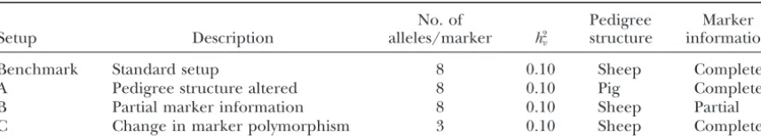
TABLE 1
Features of the four setups considered in the simulation study
No. of Pedigree Marker
Setup Description alleles/marker h2
v structure information
Benchmark Standard setup 8 0.10 Sheep Complete
A Pedigree structure altered 8 0.10 Pig Complete
B Partial marker information 8 0.10 Sheep Partial
C Change in marker polymorphism 3 0.10 Sheep Complete
1, the maternal allele of individual 6 originates from (or is tion number. Once the probabilities stabilize, the sampler is deemed to have reached convergence.
IBD to) the maternal allele of individual 1, while in the second
Two-step variance component approach:The variance com-segregation pattern, the maternal allele of individual 6
origi-ponent approach to map QTL in complex pedigrees is com-nates from (or is IBD to) the maternal allele of individual 2.
posed of two distinct steps: Therefore, based upon these realizations, Pr(6m⬅2m|Mobs)⫽
1⁄
3and Pr(6m⬅1m|Mobs)⫽2⁄3, where⬅represents IBD.
Step 1. For each QTL position on the chromosomal segment,
Multiple-site segregation sampler:A brief introduction to
the (co)variance matrix for the QTL (i.e.,G) is calcu-the multiple-site segregation sampler, as developed by
Thomp-lated. sonandHeath(1999) and employed in this article, is now
Step 2. For each position considered in step 1, construct the presented. Readers who wish to pursue a more rigorous
deriva-mixed linear models (1) and (2), obtain estimates of tion are invited to readThompsonandHeath(1999).
the parameters, and test for the presence of a QTL. Very simply, the multiple-site segregation sampler is a
clev-erly designed Gibbs sampler (GemanandGeman1984) with These steps are common to all interval mapping-based vari-batch updating, which allows IBD probabilities to be calculated ance component methods; however, their implementation dif-in pedigrees with unknown marker genotypes and unknown fers greatly among practitioners. For example, there are vari-marker phases. Exploration of the joint density Pr(s|Mobs), ous approaches to calculating theGmatrix that have already which may be of high dimension when the pedigree is large, been discussed and there are numerous analytical and simula-is facilitated through the sampling ofmsimplern-dimensional tion techniques for estimating the parameters of a mixed
conditional distributions such that linear model.
With regard to the implementation strategy adopted in this article, in step 1 the IBD probabilities for the Gmatrix are Pr(s|Mobs)⫽
兿
m i⫽1
Pr(si•|{sj•;j⬆i},Mobs), (5)
obtained via the multiple-site segregation sampler. In step 2 ASREML (Gilmouret al.1998) provides restricted maximum-wheresi•⫽{Siᐉ;l⫽1, · · · ,n} and Pr(si•|{sj•;j⬆i},Mobs) is the likelihood (REML) estimates of (1) and (2). ASREML was probability of the segregation indicators acrossnloci at the chosen over other available REML packages due to its ability ith segregation conditional on all other segregation indicators to handle large user-defined (co)variance matrices. To test and observed marker data. Since the number of loci may for the presence of a QTL against no QTL at a particular be large, drawing realizations directly from the conditional chromosomal position, the test statistic log LR⫽ ⫺2 ln(L
0(H0, distributions in (5) remains challenging. Therefore,Thomp- no QTL present) ⫺ L
1(H1, QTL present)) is constructed, sonandHeath(1999) devised a two-step strategy to sample whereL
1andL0represent the respective likelihood values of
si•from itsn-dimensional conditional distribution. (1) and (2) evaluated at the REML solutions.
The first step involves moving through the genome, calculat- Distribution of the test statistic:Statistical theory states that ing locus by locus, cumulative probabilities forSij.These proba- log LR follows a2distribution with the degrees of freedom bilities are relatively easy to calculate recursively. Once alln equal to the number of parameters being tested (Wilks1938). cumulative probabilities have been obtained, the second step However, in the context of interval mapping, the asymptotic involves moving back down the genome, samplingSijfrom a behavior of log LR is under nonstandard conditions since the
univariate density that is a function of the associated cumula- null hypothesis places parameters on the boundary of the tive probability, the previous sampled segregation indicator parameter space defined by the alternative hypothesis (Stram (Si j⫹1), and the recombination rate between locijandj⫹1. andLee1994). Furthermore, the distribution of log LR under In this way,si•can be sampled from its conditional distribution. H0 is influenced by the chromosomal segment length, the By repeating these two steps fori⫽1, . . . ,m, a realization degree of missing marker data, and the distributional
proper-from (5) is obtained. ties of the trait.
Implementation of the multiple-site segregation sampler: When a single chromosomal position is being tested, log
Implementation of the multiple-site segregation sampler is via LR follows a 50:50 mixture distribution, where one mixture an adapted version of the QTL mapping software Loki. Loki component is a peak at 0 and the other component is a2 1 was originally designed for multipoint linkage analysis in gen- distribution (Self and Liang1987). When a chromosomal eral pedigrees using MCMC methods; however, it has since interval is being tested,Xu andAtchley(1995) found the been modified for IBD probability calculation. The user sup- empirical distribution of log LR follows a2distribution with plies Loki with the pedigree structure, marker genotypes, between 1 and 2 d.f. QTL detection, however, is often carried marker positions, and QTL positions for which the IBD matri- out over large chromosomal regions and even the entire ge-ces are to be calculated. Dependent chains of IBD probabilities nome. For these situations, the distribution of log LR under are then obtained for each QTL position. Convergence is H0is unclear.
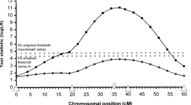
itera-Figure2.—The empirical distri-butions of log LR (from 500 repli-cates) under H0for the benchmark setup (i.e., a simulated sheep popu-lation) and setup A (i.e., a simulated pig population). (A) Locus-wide test statistic: the distribution of the test statistic when a single point on the chromosome is being tested (i.e., 35 cM). (B) Chromosome-wide test statistic: the distribution of log LR for a chromosome-wide test. The possible theoretical distribu-tions of log LR are also shown:䊏, 2
1;䉱,22; and䊉, the 50:50 mixture distribution of Self and Liang (1987).
to replicate data under the null hypothesis, construct the setup, involves the generation of fully genotyped, highly empirical distribution of log LR, and derive empirical thresh- polymorphic marker data. A biallelic QTL that explains old values in which to determine QTL presence. For real data,
10% of the total variation (i.e.,h2
v⫽0.1) is segregating
permutation methods (ChurchillandDoerge1994) have
in the population. Setups A, B, and C then change a been suggested. The large number of required analyses,
though, limits the methodology to relatively small pedigrees. single feature of the benchmark setup, enabling the Furthermore, it is not clear how the data should be permuted effect on the variance component method’s perfor-given populations with complex pedigree structures. mance to be assessed. The four setups considered in
this study are summarized in Table 1 and are discussed in detail below together with the generation of data SIMULATION STUDY
under H0.
The simulation study begins with the analysis of data Generation of data under H0:Replicates are
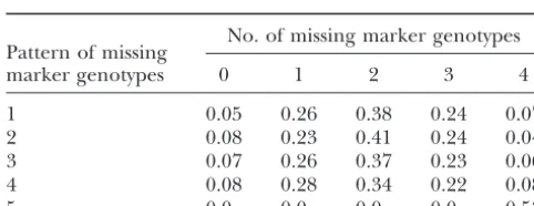
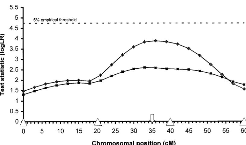
Figure3.—The mean log LR over 50 replications of data generated under the benchmark setup (i.e., sheep pedigree, biallelic QTL,h2
v⫽0.1, eight alleles
per marker, complete marker information) and setup A (i.e., pig pedigree, biallelic QTL,h2
v⫽0.1, eight
alleles per marker, com-plete marker information). 䉬and䊏, the mean log LR profile for the benchmark setup and setup A, respec-tively; 䉭, marker location;
⇓, the simulated position of the QTL.
periment contained over 2000 individuals; however, for as the midhomozygote value, a as the additive effect, anddas the dominance effect.
the purposes of demonstrating the methodology, a
sub-set of 500 individuals is selected. In reducing the pedi- The polygenic contribution made by an individual is dependent upon the polygenic contributions of its gree’s size, careful attention is given to maintaining
the structure’s original complex nature. The reduced parents and Mendelian sampling. Since the complete parentage of every individual in the pedigree is not pedigree consists of 269 related families spanning four
generations with 1.8 offspring on average per mating. available, ui is generated according to the number of
known parents. If both parents are unknown (i.e., the The pedigree structure contains no inbreeding.
The marker information consists of four polymorphic individual is a founder), then ui ⵑ N(0, 2u).
Sup-pose, however, the sire of the ith individual (si) is in
markers segregating with eight equally frequent alleles
and placed on a chromosomal segment of length 60 the pedigree. Then uiⵑ N(0.5usi, (0.75⫺0.25fsi)2u),
where fsi is the inbreeding coefficient of si. A similar
cM at positions 0, 20, 40, and 60 cM. A biallelic QTL
with allelesQandqsegregating at equal frequencies is distribution is used to generateuiwhen only the
individ-ual’s dam is in the pedigree. If both parents are present, then placed between the second and third markers at
position 35 cM. If an individual inherits QQ from its ui ⵑN(0.5(usi ⫹uDi), 0.5(1 ⫺ 0.5(fsi⫹ fDi)2u)), where
fDiis the inbreeding coefficient for the dam of individual
parents, its phenotypic contribution due to the QTL is
vi⫽m⫹a, wherem⫽0 anda⫽13.5. If the individual’s i. The environmental error termei is generated from
N(0, 2
e). Fixed effects are not generated; thus X in
QTL genotype is heterozygous or qq, the individual’s
phenotypic contribution isvi ⫽ m⫹ d orvi⫽ m⫺ a, (1) and (2) equals, the overall mean.
The value of 2
v is dependent upon m, a, d, and pQ
respectively, whered ⫽ 0.Falconer(1989) defines m
TABLE 2
Results from the analysis of data generated under the benchmark setup
Simulated Mean Mean
Parameters value estimate SD BRV bias
h2
v 0.10 0.145 0.091 0.86a 0.040
h2
u 0.34 0.296 0.127 1.03a ⫺0.039
2
e 500 488.59 65.76 0.33 ⫺4.03
dQ 35 34.48 15.64 4.31 ⫺0.91
Log LR — 4.96 4.40 0.001 —
The parameter estimates’ mean, standard deviation (SD), mean between-run variance (BRV), and mean biases forh2
v,h2u,2e, anddQare based upon 50 replicates. The mean estimate, SD, and BRV of the peak log
LR are also shown.
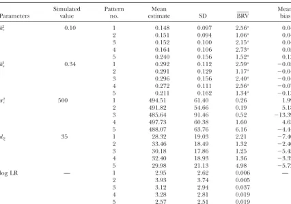
TABLE 3
Results from the analysis of data generated under setup A
Simulated Mean Mean
Parameters value estimate SD BRV bias
h2
v 0.10 0.113 0.051 0.23a 0.009
h2
u 0.34 0.324 0.119 0.19a ⫺0.022
2
e 500 496.51 56.99 1.43 6.52
dQ 35 34.23 9.22 2.05 ⫺1.09
Log LR — 12.10 7.34 0.073 —
See Table 2 for description.
aMultiply values by 10⫺5.
(the Q allele frequency), where 2
v⫽2pQ(1⫺ pQ)a2 tion of offspring that are not themselves parents. This
results in a 53% loss in marker information.
whend ⫽0 (Falconer1989). Although alteringm,a,
d, andpQaffectsv2, the size of the QTL is characterized Setup C: The final setup investigates the effect a
re-duction in marker informativeness has upon the analy-by the amount of total variation explained analy-by the QTL.
To obtain a QTL explaining 10% of the total variation, sis. Data are generated according to the benchmark setup except three alleles as opposed to eight alleles
2
uand2e are set to 300.0 and 500.0, respectively. For
these values, the heritability of the trait is 44%. are segregating at the markers.
Setup A: The ability of the variance component method to map QTL in a pedigree with large numbers
RESULTS of offspring per mating and inbreeding is investigated.
The pedigree used in this study is again based upon a Results from the application of the two-step variance component method to replicated data generated under real structure originating from a Meishan pig
experi-ment. The initial experiment containedⵑ2500 related the above-described simulation study are now reported. Due to the analyses being computationally demanding, individuals, but for meaningful comparisons to be made
with the benchmark analysis, 500 related individuals are only every third centimorgan is tested for the presence of a QTL. A single analysis across the chromosome can selected. The average number of offspring per family
is 14.3 across five generations of matings, consisting of take up to 56 min on a Compaq Professional Worksta-tion XP1000 utilizing a single Alpha 21264 processor 35 related families. The average inbreeding coefficient
is 4.5% with a maximum inbreeding coefficient of 17%. running at 500 MHz. Four parallel analyses per replicate are performed, where Loki and ASREML runs begin
Setup B:Complex pedigrees often contain individuals
with missing marker genotypes. This missing informa- from different well-dispersed starting values. The empir-ical distributions of the test statistic, however, are cre-tion introduces uncertainty into the analysis. To better
understand the ability of the methodology to cope with ated from the analysis of 500 replicated data sets; there-fore only a single run is performed per replicate due this uncertainty, two approaches to removing the
marker information generated according to the bench- to obvious computational constraints.
Construction of the empirical distribution of log LR
mark setup are explored. The first approach is where
50% of the marker genotypes are randomly removed. under H0: Figure 2A reveals close agreement between
the empirical and theoretical (i.e., 50:50 mixture where The second approach removes only the marker
informa-one compinforma-onent mixture is a peak at 0 and the other is a2
1) distributions of log LR when a single position on
TABLE 4 the chromosome is tested for QTL presence (i.e., the
35-cM position). This was found to hold regardless of
The proportion of individuals in the pedigree with 0, 1,
the position being tested.
2, 3, and 4 missing marker genotypes for patterns
1–5 in setup B In Figure 2B, when a chromosome-wide QTL search
is performed, the empirical distributions appear to fol-No. of missing marker genotypes low a 21. However, the 5% threshold value obtained Pattern of missing
from2
1 is less conservative than the empirical
thresh-marker genotypes 0 1 2 3 4
olds. The 5% empirical threshold values are 4.74 and 1 0.05 0.26 0.38 0.24 0.07 4.32 for the benchmark setup and setup A, respectively,
2 0.08 0.23 0.41 0.24 0.04 where 2
1,0.05⫽3.84. Empirical thresholds are used 3 0.07 0.26 0.37 0.23 0.06 throughout this article. It is interesting to note that the
4 0.08 0.28 0.34 0.22 0.08
empirical distributions are relatively unaffected by
5 0.0 0.0 0.0 0.0 0.53
Figure4.—The mean log LR over 50 replications of data generated under setup B (i.e., sheep pedigree, biallelic QTL,h2
v⫽
0.1, eight alleles per marker, partial marker information).䊐,䊏,⫹,䊉, *, patterns 1, 2, 3, 4, and 5 respectively. For comparison, the mean log LR of data generated under the benchmark setup is provided (䉬).䉭, marker location;⇓, the simulated position of the QTL.
Benchmark setup:The mean log LR profile over 50 amount of variation explained by the QTL. A similar result is evident inGrignolaet al.(1996b) from their replications of data generated under the benchmark
setup is shown in Figure 3. The profile peaks between simulation study. Also, the mean of the maximum log LR test statistic is 4.96, considerably larger than the peak markers 2 and 3 at the position of the simulated QTL
(i.e., 35 cM). The mean peak is well below the 5% empiri- of the mean profile given in Figure 3. This substantiates the previous claim of the mean profile being down-cal threshold; however, this result is slightly misleading.
The peak of the mean profile is biased downward be- wardly biased.
Setup A: Increasing the average family size has an cause the estimated position, and thus corresponding
peak of the profile, varies across replicates. In fact, 48% obvious effect on the performance of the methodology as evidenced in Figure 3. With larger families, the peak of the analyses yield a test statistic along the
chromo-somal segment in excess of the 5% threshold. of the log LR profile (based upon 50 replicates) in-creases from 3.9 to 11.0, where 82% of the analyses yield The ability of the methodology to accurately estimate
the parameters of interest can be gauged from the re- a log LR in excess of the 5% empirical threshold. Once again, the parameters are well estimated (see Table 3), sults presented in Table 2. The mean parameter
esti-mates ofh2
v,h2u,e2, anddQ, wheredQrepresents the loca- with mean biases slightly smaller than the biases
ob-tained under the benchmark setup. tion of the QTL in centimorgans, are close to the
simulated values; the parameter estimates’ standard de- Setup B:In setup B, five patterns of missing marker data are analyzed. Patterns 1–4 correspond to the ran-viations (SD) are reasonable; and the mean
between-run variance is small. However, a more appropriate mea- dom removal of 50% of the marker genotypes while pattern 5 is obtained by only genotyping the parents, sure of accuracy is the mean bias. The mean bias,E(ˆ⫺
), is defined as the expected value of the difference which constitutes a 53% loss in marker genotypes. The proportions of individuals in the pedigree with 0, 1, 2, between the estimator (ˆ) and the parameter’s true
value (). For example, the mean bias of the estimate 3, and 4 missing marker genotypes, for each pattern, are given in Table 4. Each pattern consists of 50 replicates. ofh2
visE(hˆ2v⫺ h2v)⫽R50i⫽1R4j⫽1[(hˆ2v)ij ⫺(h2v)i]/200, where
(hˆ2
v)ijrepresents the REML estimate ofh2vfrom the analy- These replicates, before the marker data are removed,
are the same as those replicates generated under the sis of the ith replicate and thejth parallel run, and (h2
v)i
represents the true parameter value ofh2
v. benchmark setup. Thus, differences between the results
obtained under setup B and the benchmark setup can For the parametersh2
u,2e, anddQin Table 2 the mean
bias is small and negative, implying a slight underesti- be directly attributed to the effect of missing marker information.
mating of the parameters. Forh2
v, the mean bias ofⵑ0.04
TABLE 5
Results are based upon the analysis of five different patterns of missing marker data generated under setup B
Simulated Pattern Mean Mean
Parameters value no. estimate SD BRV bias
h2
v 0.10 1 0.148 0.097 2.56a 0.044
2 0.151 0.094 1.06a 0.046
3 0.152 0.100 2.15a 0.047
4 0.164 0.106 2.73a 0.059
5 0.240 0.156 1.52a 0.134
h2
u 0.34 1 0.292 0.112 2.59a ⫺0.053
2 0.291 0.129 1.17a ⫺0.049
3 0.296 0.156 2.40a ⫺0.044
4 0.272 0.111 2.56a ⫺0.072
5 0.211 0.162 1.34a ⫺0.134
2
e 500 1 494.51 61.40 0.26 1.99
2 491.82 54.66 0.19 5.18
3 485.64 91.46 0.52 ⫺13.39
4 497.73 60.38 1.60 4.63
5 488.07 63.76 6.16 ⫺4.44
dQ 35 1 28.32 19.03 2.21 ⫺7.40
2 33.46 18.49 1.32 ⫺2.40
3 30.18 17.86 1.25 ⫺5.45
4 32.40 18.93 1.36 ⫺3.32
5 29.98 21.13 4.98 ⫺5.72
log LR — 1 2.95 2.62 0.006 —
2 3.93 3.74 0.005
3 3.12 2.94 0.037
4 3.28 2.81 0.019
5 2.57 2.51 0.019
See Table 2 for description.
aMultiply values by 10⫺5.
with the mean log LR profile for the benchmark setup mean bias forh2
vbeing more than double the mean bias
obtained under the other patterns. are shown in Figure 4. There are two points of interest
Setup C:The impact of less informative markers on to note with respect to this figure. First, the mean log
the ability of the variance component method to detect LR profile for data with partially genotyped markers
QTL is evident from Figure 5. The mean log LR profile lies below the profile obtained with complete marker
is well below the 5% threshold with only 26% of the information. Less marker information introduces extra
analyses yielding a significant peak log LR. The parame-uncertainty into the analysis and the method’s ability
ter estimates (shown in Table 6), however, are similar to detect QTL decreases. In fact, the percentages of
to the estimates obtained under the benchmark setup analyses yielding a log LR in excess of the 5% empirical
with highly informative markers. Thus, the use of less threshold are only 24, 36, 24, 28, and 20% for patterns
polymorphic markers imparts greater uncertainty into 1–5, respectively, well below the 48% achieved when the
the detection of QTL as opposed to the estimation of same data contain completely genotyped individuals.
QTL. Second, no real difference exists between the
perfor-mance of the method across patterns 1–4. However, the mean profile for pattern 5, where only the parents are
DISCUSSION genotyped, does appear to differ from the other log LR
profiles. To date, several statistical approaches have been
Figure5.—The mean log LR over 50 replications of data generated under the setup C (i.e., sheep pedigree, biallelic QTL, h2
v⫽0.1, three alleles per marker, complete marker information).䊏, the mean log LR profile for setup C. For comparison, the
mean log LR of data generated under the benchmark setup is provided (䉬).䉭, marker location; and⇓, the simulated position of the QTL.
marker information. The methodology is illustrated (co)variance matrices of v1 andv2 at two separate test positions along the chromosome. Estimates of the pa-through its application to simulated sheep and pig
pop-ulations. rameters are then obtained via ASREML and the test
statistic for the presence of two linked QTL is con-By formulating the QTL mapping problem within a
mixed linear model framework, a less parameterized structed. This process is repeated for each pair of test positions on the chromosome, enabling multiple QTL statistical environment is obtained, reducing the
compu-tational burden of the analysis. The complex relation- to be detected and localized. Note, when two QTL are being mapped, the QTL profile is a two-dimensional ships that may exist between individuals are included
within the model, leading to more accurate parameter surface.
A two-step process to estimating the variance compo-inferences, and additional fixed and random effects can
be easily incorporated into the analysis with minimal nents of a mixed linear model is not new per se.
Fer-nando and Grossman (1989), Van Arendonk et al.
adjustment to the methodology.
For example, to simultaneously map two linked QTL, (1994), andWanget al.(1995) are but a few who first calculate the IBD probabilities for the QTL’s (co)vari-the mixed linear model becomesy⫽X ⫹Zu⫹Zv1⫹
Zv2 ⫹ e, where v1 and v2 are the additive effects of ance matrix and then estimate the parameters of the mixed linear models using standard statistical tech-the linked QTL. Analogous to tech-the two-step process of
mapping a single QTL, Loki is used to calculate the niques. Difficulties in determining marker phase and
TABLE 6
Results from the analysis of data generated under setup C
Simulated Mean Mean
Parameters value estimate SD BRV bias
h2
v 0.10 0.137 0.088 1.49a 0.032
h2
u 0.34 0.287 0.133 1.70a ⫺0.048
2
e 500 493.54 60.81 2.13 0.910
dQ 35 32.21 19.66 4.29 ⫺2.94
log LR — 3.58 3.79 0.023 —
See Table 2 for description.
approximately known for chromosome (or genome)-wide scans. Questions of how missing marker genotypes, unknown marker phase, pedigree size, map density, and QTL size influence the distribution of the test statistic remain unanswered. One solution is, givenN indepen-dent tests over the chromosome (genome), calculate the (1⫺ ␣)% threshold value using the distribution of the test statistic at a single point but with the level of confidence adjusted to␣/N% (i.e., the Bonferroni cor-rection for multiple testing). See Landerand Krug-lyak(1995) for a discussion relating to the calculation ofN.An alternate solution is to further develop permu-tation testing (Churchill andDoerge 1994) so that Figure6.—The log LR profiles for a single replicate from
the trait is reshuffled in a way that destroys the associa-setup A using two different approaches to calculating the
REML estimates. The test statistics at nonmarker positions tion between QTL and trait but retains the association vary slightly due to the REML packages being run on comput- between polygenic effect and trait. It is not yet clear ers with differing machine architectures and precisions.䉬,
how this can be accomplished for complex pedigrees. the log LR profile obtained with ASREML; 䊏, the log LR
Problems also surround the construction of confi-profile obtained with the derivative-free REML package of
dence intervals for QTL position estimates. These prob-Visscher;䉭, marker location;⇓, the simulated position of the
QTL. lems are not unexpected given that the construction of
such intervals is challenging in even simple pedigrees. For an approximate confidence interval, the LOD drop-unknown marker genotypes, however, mean these off method could be employed and more accurate con-methods have limited application to populations with fidence intervals obtained under parametric and/or general pedigree structures. Via the multiple-site segre- nonparametric bootstrapping methods. However, as gation sampler, opportunities now exist to analyze data with permutation testing, resampling for nonparametric with considerably complex pedigrees. bootstrapping methods may be difficult. Clearly, further
A variety of algorithms are available for the calculation research is needed to resolve these issues.
of REML estimates. Standard algorithms such as AS- This article has been catalytic to initiating work in REML require the inverse of the QTL’s (co)variance three further areas of research. First, the simulation matrix, which is singular at marker loci. In this article, study suggests partial marker information on most
indi-Gand thus the test statistic are calculated at a position viduals is to be desired over having a mixture of fully slightly to the right or left of the marker, an approach genotyped and completely ungenotyped individuals. also adopted by I. Hoeschele (personal communica- This is currently being explored in greater detail for tion). Visscheret al. (1999) instead use a derivative- a range of missing marker scenarios. Second, a new free algorithm to calculate REML estimates that does recursive algorithm to calculate IBD probability in com-not requireG⫺1butV⫺1, whereVrepresents the
com-plex pedigrees has been developed and is currently be-plete (co)variance matrix for the likelihood. The com- ing tested. Third, the methodology is to be applied to plete (co)variance matrix is always nonsingular, allowing the analysis of real sheep and beef cattle data.
the test statistic to be calculated at marker positions. The authors thank Simon Heath for his many useful comments The two approaches give almost identical results. To and fine-tuning of Loki. This work was partly supported by a
Biotech-illustrate this, a single replicate from setup A was ana- nology and Biological Sciences Research Council award.
lyzed using ASREML and the derivative-free algorithm
of Visscheret al. (1999). The resulting QTL profiles
are shown in Figure 6. Clearly, there is little difference LITERATURE CITED between the two REML strategies; however, the present
Almasy, L.,andJ. Blangero,1998 Multipoint quantitative-trait
link-version of the derivative-free approach that calculates age analysis in general pedigrees. Am. J. Hum. Genet.62:1198–
V⫺1is considerably more computer intensive due to its 1211.
Amos, C. I., 1994 Robust variance-components approach for
as-reliance upon calculating V⫺1 for every convergence
sessing genetic linkage in pedigrees. Am. J. Hum. Genet. 54:
iterate. 535–543.
Pivotal to the success of any interval mapping proce- Cannings, C., E. A. ThompsonandM. H. Skolnick,1978 Probabil-ity functions on complex pedigrees. Adv. Appl. Prob.10:26–61.
dure is the calculation of an appropriate threshold value
Churchill, G.,andR. Doerge,1994 Empirical threshold values
in which QTL are declared significant. The threshold for quantitative trait mapping. Genetics138:963–971.
Elston, R. C.,andJ. Stewart,1971 A general model for the genetic
value is dependent upon the distribution of the test
analysis of pedigree data. Hum. Hered.21:523–542.
statistic, which is known for a single point [i.e., 50:50
Falconer, D. S.,1989 Introduction to Quantitative Genetics, Ed. 3.
mixture where one component mixture is a peak at 0 Longman Scientific and Technical, Essex, UK.
Fernando, R. L.,andM. Grossman,1989 Marker assisted selection
and the other is a2
using best linear unbiased prediction. Genet. Sel. Evol.21:467– Lin, S., E. ThompsonandE. Wijsman,1993 Achieving irreducibility
477. of the Markov chain Monte Carlo method applied to pedigree
Fulker, D. W., S. S. ChernyandL. R. Cardon,1995 Multipoint data. IMA J. Math. Appl. Med. Biol.10:1–17.
interval mapping of quantitative trait loci, using sib pairs. Am. J. Lin, S., E. ThompsonandE. Wijsman,1994 Finding noncommuni-Hum. Genet.56:1224–1233. cating sets for Markov chain Monte Carlo estimations on pedi-Geman, S.,andD. Geman,1984 Stochastic relaxation, Gibbs distribu- grees. Am. J. Hum. Genet.54:695–704.
tions and the Bayesian restoration of images. IEEE Trans. Pattern Lund, M.,andC. S. Jensen,1998 Multivariate updating of genotypes Anal. Mach. Intell.6:721–741. in a Gibbs sampling algorithm in the mixed inheritance model. George, A. W., K. L. MengersenandG. P. Davis,2000 Localisation Proceedings of the 6th World Congress on Genetics Applied to of a quantitative trait locus via a Bayesian approach. Biometrics Livestock Production Science, Vol. 25. Armidale, Australia, pp.
56:40–51. 521–524.
Geyer, C. J.,andE. A. Thompson,1995 Annealing Markov chain Male´cot, G.,1948 Les Mathe´matiques de l’He´re´dite´.Masson et Cie, Monte Carlo with applications to ancestral inference. J. Am. Stat. Paris.
Assoc.90:909–920. Self, S. G.,andK. Y. Liang,1987 Asymptotic properties of maximum
Gilmour, A. R., B. R. Cullis, S. J. WelhamandR. Thompson,1998 likelihood estimators and likelihood ratio tests under nonstan-ASREML. Program User Manual. Orange Agricultural Institute, dard conditions. J. Am. Stat. Assoc.82:605–610.
New South Wales, Australia. Sheehan, N.,1990 Genetic restoration on complex pedigrees. Ph.D. Grignola, F. E., I. HoescheleandB. Tier,1996a Mapping quanti- Thesis, University of Washington, Seattle.
tative trait loci in outcross populations via residual maximum Stram, D. O.,andJ. W. Lee,1994 Variance component testing in likelihood. I. Methodology. Genet. Sel. Evol.28:479–490. the longitudinal mixed effects model. Biometrics50:1171–1177. Grignola, F. E., I. Hoeschele, Q. ZhangandG. Thaller,1996b Thompson, E. A.,1994 Monte Carlo estimation of multilocus
autozy-Mapping quantitative trait loci in outcross populations via
resid-gosity probabilities. Proceedings of the 1994 Interface Confer-ual maximum likelihood. I. A simulation study. Genet. Sel. Evol. ence, Fairfax Station, VA, pp. 498–506.
28:491–504.
Thompson, E. A.,andS. C. Heath,1999 Estimation of conditional Grignola, F. E., Q. ZhangandI. Hoeschele,1997 Mapping linked
multilocus gene identity among relatives, pp. 95–113 inStatistics quantitative trait loci via residual maximum likelihood. Genet.
in Molecular Biology, edited byF. Seillier-Moseiwitch, P. Don-Sel. Evol.29:529–544.
nellyandM. Waterman.Springer-Verlag IMS lecture note se-Heath, S. C.,1997 Markov chain Monte Carlo segregation and
ries, New York. linkage analysis for oligogenic models. Am. J. Hum. Genet.61:
Uimari, P.,andI. Hoeschele,1997 Mapping two linked quantitative 748–760.
trait loci using Bayesian analysis and Markov chain Monte Carlo Hoeschele, I.,1993 Elimination of quantitative trait loci equations
algorithms. Genetics146:735–743. in an animal model incorporating genetic marker data. J. Dairy
Van Arendonk, J. A. M., B. TierandB. P. Kinghorn,1994 Use Sci.76:1693–1713.
of multiple genetic markers in prediction of breeding values. Hoeschele, I., P. Uimari, F. E. Grignola, Q. ZhangandK. M. Gage,
Genetics137:319–329. 1997 Advances in statistical methods to map quantitative trait
Visscher, P. M., C. S. Haley, S. C. Heath, W. J. MuirandD. H. R. loci in outbred populations. Genetics147:1445–1457.
Blackwood,1999 Detecting QTLs for uni and bipolar disorder Jansen, R. C., D. L. JohnsonandJ. A. M. Van Arendonk,1998 A
using a variance component method. Psych. Genet.9:75–84. mixture model approach to the mapping of quantitative trait loci
Wang, T., R. L. Fernando, S. Van Der Beek, M. Grossmanand in complex populations with an application to multiple cattle
J. A. M. Van Arendonk,1995 Covariance between relatives for families. Genetics148:391–399.
a marked quantitative trait locus. Genet. Sel. Evol.27:251–274. Jayakar, S. D.,1970 On the detection and estimation of linkage
Wilks, S. S.,1938 The large sample distribution of the likelihood between a locus influencing a character and a marker locus.
ratio for testing composite hypotheses. Ann. Math. Stat.9:60–62. Biometrics26:451–464.
Xie, C., D. G. GesslerandS. Xu,1998 Combining different line Jensen, C. S.,andH. Sheehan,1998 Problems with determination
of noncommunicating classes for Monte Carlo Markov chain crosses for mapping quantitative trait loci using the identical by applications in pedigree analysis. Biometrics54:416–425. descent-based variance component method. Genetics149:1139– Knott, S. A., J. M. ElsenandC. S. Haley,1996 Methods for multi- 1146.
ple-marker mapping of quantitative trait loci in half-sib popula- Xu, S.,andW. R. Atchley,1995 A random model approach to tions. Theor. Appl. Genet.93:71–80. interval mapping of quantitative trait loci. Genetics141:1189– Lander, E.,andL. Kruglyak,1995 Genetic dissection of complex 1197.
traits: guidelines for interpreting and reporting linkage results.