Targeted Graph Mining for Efficient User-Relevant Knowledge Discovery.

(1)

ABSTRACT

HARENBERG, STEVEN DOUGLAS. Targeted Graph Mining for Efficient User-Relevant Knowledge Discovery. (Under the direction of Dr. Nagiza F. Samatova.)

Mining for user-relevant knowledge from large-scale graph data is at the core of graph data analytics in applications spanning many domains, such as biomedical informatics, social network

analysis, and climate science. These applications can often benefit from a targeted enumeration

of specific graph substructures, where the output is constrained or influenced by user preferences. For example, a user may only be interested in substructures containing genes known to be

associated with Alzheimer’s disease. These genes could be viewed as the user’s knowledge priors

or query vertices.

Targeted graph mining, as introduced in this thesis, aims to help prevent enumerating

undesirable or irrelevant patterns and aims to generate output that better relates to the user’s

preference. Moreover, it can reduce both the computational requirements of the enumeration process as well as the human effort involved in analyzing the results. For example, even if the

number of enumerated substructures grows linearly with the graph size, it becomes impossible to

manually inspect each substructure for value added to the application knowledge base. Therefore, we posit that targeted algorithms incorporating knowledge priors and user preferences can help

facilitate an exploratory and interactive approach towards mining user-relevant knowledge from

graph data.

In this dissertation, we explore targeted graph mining algorithms in the context of clique and

community detection. In our first component, we propose two memory efficient algorithms for

enumerating cliques that are enriched by user-specified knowledge priors. These complementary algorithms consist of a top-down precomputation and index-based method and a bottom-up

method. We evaluate the efficiency of our algorithms on a number of real-world networks and

demonstrate the practical value by mining a protein interaction network with Alzheimer’s Disease biomarkers as the knowledge priors.

In our second component, we develop a hybrid approach to the complementary top-down and bottom-up algorithms. With our approach, we are able to develop a synergy between successive

queries over the same graph by designing a state space indexing and querying strategy. By

dynamically indexing the constituent state space generated with each query, this strategy is able to reduce redundant computations from similar queries and promote targeted exploration

of user-relevant substructures. Experimental results over real-world networks demonstrate our

strategy’s effectiveness at reducing cumulative query-response time.

Finally, we shift our focus towards enabling a framework for mining user-relevant substructures

(2)

methods. Our third dissertation component, a comprehensive survey and evaluation on the

recent advances in this body of literature, has motivated the idea that developing this framework to be adaptable to the user’s desired community detection method is important, as each method

may have strengths and weaknesses for different applications. Therefore, in our final component,

(3)

(4)

Targeted Graph Mining for Efficient User-Relevant Knowledge Discovery

by

Steven Douglas Harenberg

A dissertation submitted to the Graduate Faculty of North Carolina State University

in partial fulfillment of the requirements for the Degree of

Doctor of Philosophy

Computer Science

Raleigh, North Carolina

2017

APPROVED BY:

Dr. R. Raju Vatsavai Dr. Kemafor Anyanwu Ogan

Dr. Dennis R. Bahler Dr. Nagiza F. Samatova

(5)

DEDICATION

(6)

BIOGRAPHY

Steve Harenberg obtained a Bachelor of Science in Mathematics and minor in Computer Science from the University of North Carolina in 2011. He entered North Carolina State University’s

Graduate Program in the fall of 2012 with Dr. Nagiza Samatova as his advisor. During his doctoral study, Steve had a research aide appointment at Argonne National Laboratory and an

(7)

ACKNOWLEDGEMENTS

The support and guidance from many people and institutions were integral towards my completion of this dissertation. First and foremost, I would like to thank my research advisor Dr. Samatova,

her wisdom, guidance, and support were critical towards helping me grow as a researcher. I would also like to extend my gratitude to various faculty members of the Computer Science

department at North Carolina State University. In particular, I would like to thanks the members

of my PhD committee, Dr. Raju Vatsavai, Dr. Dennis Bahler, and Dr. Kemafor Ogan, for their valuable time in serving on my graduate committee and for their insightful suggestions regarding

my dissertation. I would also like to thank Dr. Rada Chirkova for her guidance and input at the

beginning of my PhD and particularly with the first two components of my dissertation. I have also been fortunate to have valuable collaborations with researchers at other institutions.

I would like to thank Tom Peterka at Argonne National Lab for his guidance while I was a

research aide over a summer and Kelly Holohan at Indiana University for her help with the biological analysis of our results in Chapter 2.

In addition, I have received a tremondous amount of support from the other students of Dr.

Samatova’s group, so I would like to extend my gratitude to Gonzalo Bello, Mandar Chaudhary, Stephen Ranshous, Ramona Seay, Jitendra K. Harlalka, Kanchana Padmanabhan, David “Drew”

Boyuka, Lucia Gjeltema, and Sriram Lakshminarasimhan.

Finally, I would like to especially thank my family for their love and support over the years. This dissertation is based upon work supported in part by the Laboratory for Analytic

Sciences (LAS), the DOE SDAVI Institute, the U.S. National Science Foundation (Expeditions

in Computing program), and the NSF grant 1029711. Any opinions, findings, conclusions, or recommendations expressed in this dissertation are those of the author and do not necessarily

(8)

TABLE OF CONTENTS

LIST OF TABLES . . . vii

LIST OF FIGURES . . . .viii

Chapter 1 Introduction . . . 1

1.1 Targeted Graph Mining . . . 2

1.1.1 Mining Enriched Cliques . . . 4

1.1.2 Dynamic State-Space Indexing . . . 5

1.1.3 Community Detection: Comparative Analysis . . . 5

1.1.4 Cross-Graph Community Mining . . . 5

Chapter 2 Mining Enriched Cliques . . . 7

2.1 Introduction . . . 7

2.2 Related Work . . . 8

2.3 Problem Statement . . . 9

2.4 Background . . . 10

2.5 Bottom-up Algorithm . . . 11

2.5.1 Enrichment-Aware Pivoting . . . 13

2.5.2 Memory Utilization . . . 14

2.5.3 Correctness Proof . . . 14

2.6 Index-Based Algorithm . . . 16

2.6.1 Precomputation and Indexing . . . 16

2.6.2 Querying . . . 17

2.6.3 Memory Utilization . . . 20

2.6.4 Correctness Proof . . . 20

2.7 Results . . . 21

2.7.1 Reducing Computation . . . 23

2.7.2 Bottom-up vs. Index-based . . . 24

2.7.3 Comparison with DENSE . . . 25

2.8 Disease Associations . . . 27

2.8.1 Identifying Gene-Disease Associations . . . 27

2.8.2 Identifying Disease-Disease Associations . . . 28

2.9 Conclusion . . . 30

Chapter 3 Dynamic State-Space Indexing . . . 32

3.4 Biased Clique Search . . . 35

3.5 Index and Query . . . 37

3.5.1 Storing and Indexing the Search Space . . . 37

3.5.2 Query processing . . . 38

(9)

3.6.1 Benefits of Dynamic Indexing . . . 40

3.6.2 Computational Overhead of Dynamic Indexing . . . 42

3.6.3 Application: Climate Science . . . 43

Chapter 4 Community Detection: Comparative Analysis . . . 45

4.3 Algorithms . . . 47

4.3.1 Overlapping Community Detection . . . 47

4.3.2 Disjoint Community Detection . . . 49

4.4 Methodology . . . 51

4.4.1 Datasets . . . 52

4.4.2 Parameter Selection . . . 54

4.4.3 Goodness Metrics . . . 54

4.4.4 Performance Metrics . . . 55

4.5 Results . . . 55

4.5.1 Goodness Metrics Results . . . 55

4.5.2 Performance Metrics Results . . . 59

4.5.3 Similarity Measure . . . 62

4.5.4 Run-Time . . . 63

Chapter 5 Cross-Graph Community Mining . . . 65

5.4 Methods . . . 68

5.4.1 CC-Tree Structure . . . 68

5.4.2 Persistent Communities . . . 71

5.4.3 Discriminative Communities . . . 73

5.4.4 Query Support . . . 76

5.5 Results . . . 77

5.5.1 Ordering the CC-Tree . . . 78

5.5.2 Persistent Community Enumeration . . . 80

5.5.3 Discriminative Enumeration . . . 82

5.5.4 Discriminative Optimization . . . 83

Chapter 6 Conclusion . . . 85

6.1 Future Work . . . 86

(10)

LIST OF TABLES

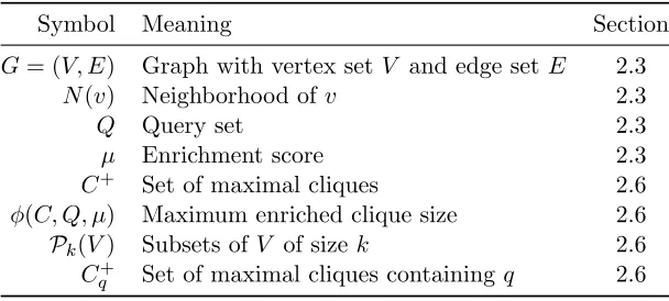
Table 2.1 Notation summary . . . 10

Table 2.2 Synthetic graph properties . . . 22

Table 2.3 Diseases having high association scores with Alzheimer’s . . . 30

Table 4.1 Community detection algorithms evaluated. . . 47

Table 4.2 Summary of the graphs used for the evaluations. . . 53

Table 4.3 Best and worst algorithms for each goodness and performance metric. . . . 59

Table 4.4 Performance metrics for overlapping community detection. Results displayed asmedian [range] over ten runs where applicable. . . 60

Table 4.5 Performance metrics for disjoint community detection. Results displayed asmedian [range] over ten runs where applicable. . . 61

(11)

LIST OF FIGURES

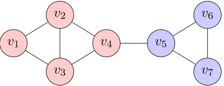
Figure 1.1 Example protein functional association network with vertices correspond-ing to proteins (labeled by the name of its encodcorrespond-ing gene) and an edge between two proteins if there is substanial evidence suggesting those two proteins are functionally associated [80]. . . 2 Figure 1.2 Example graph containing four maximal cliques: {v1, v2, v3},{v2, v3, v4},

{v4, v5},{v5, v6, v7}. In terms of communities, most algorithms would

prob-ably partition the graph into two groups, such as {v1, v2, v3, v4},{v5, v6, v7}. 3

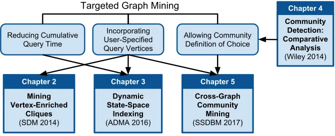
Figure 1.3 Overview of the dissertation chapters how they relate to the research objectives. . . 4

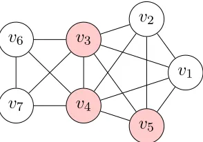
Figure 2.1 Example graph with query set Q={v3, v4, v5}. For an enrichment of µ=

3/5 there are three maximal biased cliques: {v1, v2, v3, v4, v5}, {v3, v4, v6},

and {v3, v4, v7}. . . 9

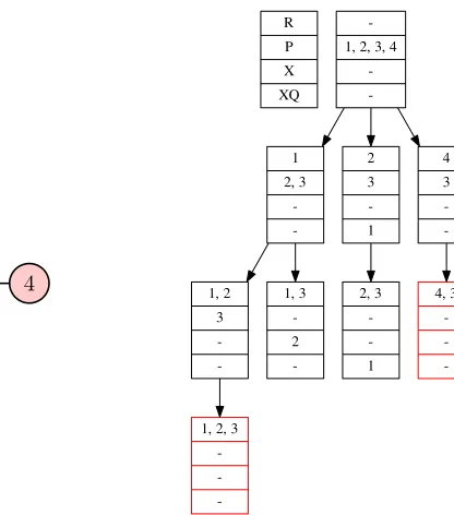
Figure 2.2 Simple graph and example search space generated by Algorithm 2.2 with query (Q={1,2,4}, mu= 0.5. Red states represent the output cliques. . 13 Figure 2.3 Example of a graph with its corresponding indices for vertex and clique

mappings. The vertex to clique mapping allows us to quickly look up all cliques containing query vertices (highlighted in red). The clique to vertex mapping allows us to look up the actual values of a clique. . . 16 Figure 2.4 Given Q = {3,5} and µ = 1/3, the set {1,3,4} is locally maximal µ

-enriched within the first clique, but not maximal in the entire graph. . . . 17 Figure 2.5 The reduction of computation from our enrichment-aware pivoting

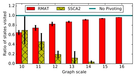
tech-nique in the bottom-up algorithm with µ= 0.1 and|Q| ≈0.01|V|. Note that only sizes up to 214 were run for the SSCA2 graphs due to time constraints particularly with the non-pivoting algorithm. . . 23 Figure 2.6 The reduction of subset checks achieved by our technique of using a set

X to keep track of visited vertices. These queries were run withµ= 0.25 and |Q| ≈0.01|V|. . . 24 Figure 2.7 Run time and output size using random sets of query vertices at four

different sizes over the Stanford communication/email graph. Each query size is based on the number of vertices in the graph, which was |V|= 265,009. For this experiment,µ was set to 0.5. . . 24 Figure 2.8 Run-time performance and peak memory usage of the index-based and

bottom-up method for varying µ values on several SNAP (unfilled points) and R-MAT (filled points) graphs. Ratios for index-based are circles and ratios for bottom-up are triangles. A missing data point means that the algorithm timed out (>10 min). All possible points can be seen in the graphs for µ= 0.75. . . 25 Figure 2.9 Speedup and peak memory usage ratio of the index-based and

(12)

Figure 3.1 An example graph with eight maximal cliques. For a query (Q={1,2}, η = 2), there are two biased maximal cliques,{1,2,3}and {1,2,6}. . . 34 Figure 3.2 Search space when mining all maximal cliques of the graph in Figure 3.1.

Gray nodes show the search space out of the total space (gray and white) that would be visited when mining biased cliques with query (Q={1,2}, η = 2). The rows in each node correspond to the sets R, P, and X, respectively. Note that this tree does not show pivoting. . . 37 Figure 3.3 Query process with query vertices Q={4,5} and bias η = 2. Here, we

assume that the red-outlined states of Figure 3.2 are indexed. The states in the inverted Indexof each query vertices have theirCountincremented inH. Then, theStateswhose counts inHare at leastη are fed toSearch to produce Output. . . 38 Figure 3.4 Cumulative run-time efficiency of our dynamic state space index compared

to the baseline methods (Full and None) when performing a number of queries (with bias valueη = 4 and query size|Q| ≈0.01|V|) on the Pokec graph. . . 41 Figure 3.5 Compared to no index (None), our dynamic state space index (Dynamic)

allows for much fewer states to be expanded. This plot shows 100 queries (withη= 2 and query size |Q| ≈0.001|V|) on the Pokec graph for three cases involving 0%, 50%, and 90% overlap between successive queries. . . 41 Figure 3.6 Time spent for our dynamic indexing strategy. For queries on Epinions

covering a complete search space, there is no overhead compared to Full. For queries on Pokec covering only small subset of the search space, there is only a small overhead compared to None. Each plot is labeled with (bias valueη, query size as fraction of |V|). . . 42 Figure 3.7 Cliques biased towards the MDR and known climate indices associated

with Atlantic hurricane variability. . . 43

Figure 4.1 Goodness metrics for overlapping community detection. Missing boxplots indicate that the corresponding algorithm did not finish on that graph within four hours. . . 56 Figure 4.2 Goodness metrics for disjoint community detection. Missing boxplots

indicate that the corresponding algorithm did not finish on that graph within four hours. . . 57 Figure 4.3 Matrices of pairwise similarity scores for the community detection

algo-rithms and the ground-truth. Dots indicate that a similarity score could not be computed, because one of the algorithms did not finish on that graph within four hours. . . 63 Figure 4.4 Run-times of the disjoint and overlapping community detection algorithms

(including read and write times) per graph. The algorithms were terminated if they did not finish within four hours. For the nondeterministic algorithms, the average of ten run-times was taken. . . 64

(13)

Figure 5.2 Number of states generated during our method when ordering the vertices in the CC-Trees based on the total vertex counts or vertex supports. . . . 79 Figure 5.3 Runtime of our method compared to the baselineαβ-clique when varying a

number of different parameters. Except for the parameter being analyzed, the values are set to |V|= 16000,α= 5, |G|= 10, and fraction of vertex swaps to 0.2 . . . 81 Figure 5.4 Runtime of our method compared to the baseline αβ-clique when varying

the minimum positive class support threshold α and maximum negative class support threshold β. Each threshold was varied once and controlled once, as a control the threshold was set to 5, which was half the size of the graph ensemble. The right figure shows the runtime for the three components of our framework. . . 83 Figure 5.5 Runtime and information gain comparison of our MDCF method with two

(14)

CHAPTER

1 INTRODUCTION

Graphs, or networks, are a ubiquitous way to model complex systems in a variety of scientific domains, such as biology, climate science, and sociology. Graphs represent objects with vertices (or nodes) and interactions between those objects as edges. The physical interpretation of the vertices and edges will depend on the particular domain at hand. For example, in biology, a protein functional association networks may model the association of hundreds of thousands

proteins based on different evidences [80], a small example of which is illustrated in Figure 1.1.

On the other hand, in climate science, a network may model similarly correlated regions of Earth based on some important metric, like sea surface temperature [78].

Mining for substructures in these networks can help illuminate the underlying mechanisms

of the physical system. For example, identifying groups of highly connected vertices in a protein-protein interaction network, referred to as functional modules, can help determine the

functional organization of cells [2]. This same substructure in a climate network may correspond

to homogenous climate regions that can be used as a comparison metric for different climate models [77].

In applications such as these, rather than enumerating all substructures of a specific type, the user may be interested in a smaller, targeted subset of the output space, one that is more relevant

to their application at hand. For example, the user may be only interested in substructures

(15)

Figure 1.1 Example protein functional association network with vertices corresponding to proteins (labeled by the name of its encoding gene) and an edge between two proteins if there is substanial

evidence suggesting those two proteins are functionally associated [80].

these genes or climate indices can be consideredquery vertices or knowledge priors.

1.1 Targeted Graph Mining

Targeted graph mining, as introduced in this thesis, allows the user to perform a targeted

enumeration process based on their preferences or knowledge priors. This provides a twofold

benefit. First, the output better relates to the interests of the user, which means they do not have to sift through a large output space that would be difficult to manually inspect otherwise.

Second, the computational requirements of the enumeration process can be reduced, improving efficiency. As a result, we posit that targeted algorithms incorporating knowledge priors and

user preferences can help facilitate an exploratory and interactive approach towards mining

user-relevant knowledge from graph data.

In this thesis, we explore targeted graph mining algorithms in the context of clique and

community detection. As illustrated by the examples above, discovering groups of highly

connected vertices is a graph mining task that translates across a number of scientific domains. Amongst others, one substructure that embodies this property is the clique. A clique is a set of vertices that are pairwise connected; i.e., every node is connected to every other node. Due to

the importance of cliques a variety of applications, as well as their interesting mathematical properties, a number of methods have been explored for enumerating all the maximal cliques

(16)

v

1

v

2

v

3

v

4

v

5

v

6

v

7

Figure 1.2 Example graph containing four maximal cliques:{v1, v2, v3},{v2, v3, v4}, {v4, v5}, {v5, v6, v7}. In terms of communities, most algorithms would probably partition the graph into two

groups, such as{v1, v2, v3, v4},{v5, v6, v7}.

illustrated in Figure 1.2.

In addition, a more general class of substructures–communities–are also useful for a variety of applications. Communities can be thought of a parent class of substructures of which a clique

may be considered a baseline case or simple instance. There is no formal definition for what constitutes a community, though communities are informally thought of as densely connected

groups of nodes that are sparsely connected to the rest of the network (see Figure 1.2). There

are a number of structural metrics related to this definition, such as conductance or modularity, but in many cases communities are just algorithmically defined [25]; i.e., an algorithm intuitively

tries to break-up the graph into groups that capture notion of communities.

Overwhelmingly, the research in these areas focuses on algorithms that output all instances of a specific substructure, leaving little control to the user. Therefore, in this thesis, we address

the need for targeted graph mining algorithms by exploring a few research objectives in the

context of clique and community mining:

1. Developing algorithms that can incorporate query vertices to mine more user-relevant substructures.

2. Reducing cumulative query time to promote exploratory knowledge discovery, where a user may wish to perform multiple queries for substructures containing different vertices

of interest.

3. Allowing the user to choose their community definition of choice for cross-graph

substruc-ture mining.

Figure 1.3 illustrates how the chapters of this dissertation relate to the above research objectives. Our second chapter [34] focuses on both objectives in the context of clique enumeration, as

cliques are a formally defined structure that provides a good foundation to begin building our

(17)

Cross-Graph Community

Mining (SSDBM 2017)

Chapter 5

Dynamic State-Space

Indexing (ADMA 2016)

Chapter 3

Mining Vertex-Enriched

Cliques (SDM 2014)

Chapter 2

Community Detection: Comparative

Analysis (Wiley 2014)

Chapter 4

Incorporating User-Specified Query Vertices Reducing Cumulative

Query Time

Allowing Community Definition of Choice Targeted Graph Mining

Figure 1.3 Overview of the dissertation chapters how they relate to the research objectives.

the indexing strategy with a dynamic approach that indexes in a more targeted manner to

reduce cumulative query response time. Our fourth chapter [32] performs a comparative analysis of community detection approaches and forms the motivation of our final chapter [35], where

we develop a top-down method for mining communities across an ensemble of graphs based on

some structural definition of community chosen by the user.

1.1.1 Mining Enriched Cliques

Most clique or community enumeration methods generally focus on full enumeration, though a

limited number of methods have explored incorporating query nodes, typically either finding a single community that contains a set of query nodes [76, 84], or all the communities that contain a single query node [21, 22]. However, there are more complex ways that that knowledge prior

query vertices could be incorporated, such as ensuring that some minimum percentage of the substructure consists of query nodes or ensuring that there are a least some minimum number

query nodes in the substructure.

In Chapter 2, we explore two complementary strategies for targeted clique enumeration: a top-down approach and a bottom-up approach. In the top-down approach, we perform a large

precomputation step to first mine and index all cliques in the graph. The index is then used to

answer subsequent user-queries. In the bottom-up approach, we incorporate the knowledge priors directly into the enumeration process to only generate cliques that are relevant to the knowledge

priors. We evaluate the efficiency of our proposed techniques on a number of real-world and

synthetic networks. Moreover, to demonstrate the practical value of our approach, we use our methods to uncover gene-disease associations by mining a protein functional association graph

(18)

1.1.2 Dynamic State-Space Indexing

In some cases, a user may want to mine the graph in an exploratory manner, probing with different, but perhaps related, knowledge prior sets over a number of queries. For example, the

user may wish to mine functional modules relevant to Alzheimer’s-associated genes as well as

functional modules relevant to Diabetes-associated genes. In situations like these, the user may not be exploring enough of the entire search space to warrant the large precomputation time

required to build a full index. However, repeatedly using a bottom-up approach for multiple

queries will likely produce redundant computation between successive queries (e.g., a query for patterns containing u and v, and a query for patterns containing uand w). Most importantly, with both of these strategies, there is no synergy between successive queries despite the possibility

of some computational overlap in the search space.

Therefore, in Chapter 3, we develop a strategy that facilitates exploratory knowledge

discovery by reducing the cumulative query response time. The key idea is to store and index the constituent state space generated with each query. Subsequent queries can then leverage

this index to avoid recomputing any parts of the search space previously generated. Moreover,

the index is incrementally updated as more queries are performed, thereby generating and storing exactly the query-relevant search space. We evaluate our strategy over several real-world

networks and various query scenarios to demonstrate its effectiveness at reducing the cumulative

query response time.

1.1.3 Community Detection: Comparative Analysis

In Chapter 4, we begin further exploring the abundance of other community definitions and

methods. Community detection is one of the most widely researched problems in graph data analytics; therefore, in this chapter, we perform a comparative analysis of state-of-the-art

community detection techniques to survey the field. The survey focuses on a comparative

analysis of state-of-the-art community detection methods over several real-world networks. Importantly, the real-world networks had known ground-truth communities, allowing us to

perform our comparisons via various performance (e.g., precision, recall, etc.) and goodness (e.g.,

density, conductance, etc.) metrics. We compared both disjoint community detection techniques, where every node can only belong to one community, as well as overlapping community detection

techniques, where nodes can belong to multiple communities. Through this process, were were

able to identify some research directions motivating the final chapter of this dissertation.

1.1.4 Cross-Graph Community Mining

As mentioned above, communities are a more general class of substructures that are also highly

(19)

data as an ensemble of graphs; for example, graph ensembles can be created from multiple: social

networks at distinct points in time, biological networks created from independent experiments, and global climate networks created from unique climate models.

Therefore, in Chapter 5, we focus on the problem of finding subcommunities that persist

across a collection of graphs or that discriminate between two classes of graphs. For example, the user may be interested in discovering functional modules that discriminate between people

with some disease and people without that disease as a way to help understand the underlying

mechanisms. While there is work on discriminative subgraphs analysis [42], there are few methods that mine specific structures, such as communities.

As there are no single “best” community detection technique or definition, our guiding

priciniple is designing a top-down framework that that is adaptable to different community detection methods as targeted by the user. This will enable the user to take advantage of the

abundance of community detection techniques most relevant to their application at hand. In

(20)

CHAPTER

2 MINING ENRICHED CLIQUES

2.1 Introduction

Maximal clique enumeration (MCE), a long-standing graph pattern enumeration task. MCE methods can be used for various applications, such as enumerating densely connected subnetworks

in large protein-protein interaction graphs [96], discovering social hierarchy in email networks [20],

and identifying regions of homogeneous long-term climate variability in climate networks [78]. However, it is often the case that only a subset of cliques from the entire set is of interest to the

end-user given his/her target problem. For example, only genes that are functionally associated

with Alzheimer’s (AD) biomarker genes must be detected from the human genome-scale network for subsequent manual curation and literature evidence support. Such biomarker genes in the

network could be viewed as knowledge priors, or query nodes, and the generic problem of clique enumeration is thus reduced to query-driven clique enumeration. Arguably, targeted clique enumeration with knowledge priors could produce output that better relates to the user’s

preference, avoid enumerating undesirable cliques, and reduce computation.

(21)

invocations of the algorithm with different parameters to identify more than one community of

interest. The second way requires not only multiple algorithm runs to cover all query nodes but also post-processing removal of duplicate communities. The third way addresses the limitations

of the other two and provides an end-user the flexibility to balance the specificity and the

sensitivity of the desirable associations with knowledge priors. As a result we will focus on this last way of incorporating knowledge priors.

In this chapter, we explore two memory efficient methods for mining vertex-enriched cliques.

The main contributions of this chapter are as follows:

1. An bottom-up algorithm (Section 2.5) and the underlying theory for enumerating cliques that are “enriched” by a set of query nodes. This approach incorporates knowledge priors

directly into the enumeration process in a DFS manner to maintain a low peak memory

profile. We also develop an enrichment-aware pivoting technique to reduce the size of the search space.

2. An index-based method (Section 2.6) and the supporting theory that provide a foundation

for enriched clique enumeration as a post-processing step after cliques have been

pre-computed. This method operates in a top-down manner on a single clique at a time to achieve a low memory overhead. We develop techniques to completely eliminate the need

for superset checks and reduce the number of subset checks, two challenges that arise from

mining enriched cliques in a top-down manner.

3. Identification Alzhiemer’s associated genes when using our method to mine a protein-protein functional assocation network with known Alzheimer’s biomarkers (Section 2.8).

2.2 Related Work

This work is closely related to (quasi-)clique enumeration and overlapping community detection. Although these fields have been well studied, the vast majority of this research has been focused

on methods for enumeratingall communities or clique structures in a graph. To the best of our knowledge, few works have studied a query-driven variant of these problems.

Sozio et al. [76], and later Tsourakakis et al. [84], define a query-driven dependent version

of the overlapping community problem, which is termed the community search problem. This

version of the problem takes a query set Q as input, in addition to the graph, and seeks to find the optimal subgraph H ⊇Q that maximizes some scoring function. A similar problem was formulated by Andersen et al. [5], which looked to expand a set of seed vertices into its

(22)

v

1

v

2

v

3

v

4

v

5

v

6

v

7

Figure 2.1 Example graph with query setQ={v3, v4, v5}. For an enrichment ofµ= 3/5 there are

three maximal biased cliques:{v1, v2, v3, v4, v5},{v3, v4, v6}, and{v3, v4, v7}.

all the communities that contain that vertex. In contrast, in this work we are using the definition

proposed by Hendrix et al. [36] that bridges these two extremes and extracts all cliques that contain a minimum percentage of vertices fromQ.

DENSE, a method for solving this problem for quasi-cliques, is highly memory-intensive

and cannot scale to large graphs due to needing to store the output in memory for subset checking. In fact, DENSE, along with many current approaches in community detection and

clique enumeration are not memory conscious. However, Cheng et al. [16] proposed a scalable

version of MCE that only operates on limited sized subgraphs in memory at any given time, though it does not incorporate knowledge priors.

2.3 Problem Statement

In the case of cliques, knowledge priors, or vertices of interest, could be incorporated into the enumeration process in a couple of ways. Here, we will focus on enumerating cliques such that

some percentage of nodes that makeup the clique are the knowledge prior query vertices. We

will refer to this as maximal enriched clique enumeration (MECE). More formally, we introduce the following definitions:

Definition 2.1. Given a graph G= (V, E), a query set of vertices Q ⊆V, and a real value

µ∈ (0,1], a clique C ⊆V is a µ-enriched clique in G with respect to Q if at least dµ|C|e

vertices ofC are in Q.

Given this definition, we refer to the ordered pair (Q, µ) as the user-specifiedquery. Moreover, as is consistent with its usual usage, an enriched clique is said to bemaximal if it is not contained in a larger clique that is also enriched. See Figure 2.1 for an example of these two types of

cliques. This leads us to the following problem statement that will be the focus of this chapter.

Problem 2.1. Given a simple, undirected graph G= (V, E) and a query (Q, η), enumerate all

(23)

Table 2.1 Notation summary

Symbol Meaning Section

G= (V, E) Graph with vertex set V and edge set E 2.3

N(v) Neighborhood of v 2.3

Q Query set 2.3

µ Enrichment score 2.3

C+ _{Set of maximal cliques} _2.6

φ(C, Q, µ) Maximum enriched clique size 2.6

P_k(V) Subsets of V of sizek 2.6

C+

q Set of maximal cliques containing q 2.6

Note that a maximal enriched clique may not correspond to a maximal clique. That is, there could be a maximal enriched clique that is a subset of a clique. Consider the example show in

Figure 2.1, and suppose we had µ= 2/3, meaning 2/3 of the vertices in the clique must be in Q. Then, {v3, v4, v6} and {v3, v4, v7} would both be maximal enriched cliques, and both of these

are subsets of the maximal (not enriched) clique{v3, v4, v6, v7}.

Finally, Table 2.1 summarizes the notations used in this chapter with the number of the

section where they are defined.

2.4 Background

To mine enriched and biased cliques, we will be leveraging strategies from a well-known MCE algorithm by Bron and Kerbosch (BK) [13] as it is is arguably one of the best overall performing

MCE algorithms (especially considering its simplicity). The BK algorithm, as detailed in

Algorithm 2.1, is an enumerative backtracking algorithm that finds maximal cliques by growing all possible cliques one vertex at a time. When a clique cannot be made any larger, it is output

as a maximal clique (lines 1-2). Each state in the search tree of the BK algorithm consists of

three sets of vertices (R, P, X) whereRrepresents the current clique being computed, P defines candidate vertices that may be added toR, andX defines vertices that must be excluded from R to prevent a redundant state from occurring. As such, any maximal clique generated by a state (R, P, X) must be a subset ofR∪P.

The algorithm performs a depth-first search through the search tree, adding a candidate

(24)

Algorithm 2.1: BK(maximal clique enumeration [13]) input :Graph G= (V, E)

Vertex sets R,P,X ⊆V output :Maximal cliques in Gfrom P

1 if setsP and X are both emptythen 2 OutputR as a maximal clique 3 Select a pivot vertex u fromP ∪X 4 for vertexv∈P\N(u) do

5 BK(R∪ {v}, P ∩N(v), X∩N(v))

6 P ←P\ {v}

7 X←X∪ {v}

algorithm is initially called withR=X=∅ and P =V.

2.5 Bottom-up Algorithm

The algorithm described in this section is an enumerative backtracking algorithm that builds cliques one vertex at a time. We incorporate query vertices (knowledge priors) directly into the

enumeration process so that no cliques unrelated to the query are constructed. Like the BK

algorithm, we use a DFS approach when exploring the search space to maintain a reasonable memory profile.

Like the BK algorithm, we keep track of sets of vertices that represent different aspects of

our current state in the search space. We use the same three sets from the BK algorithm in addition to an extra state XQ. These states are summarized as follows:

• R: Set of vertices forming a µ-enriched clique (may or may not be maximal).

• P: Candidate set of vertices that could expandR such that∀v∈P, v /∈R and∀u∈R, v∈

N(u).

• X: Set of non-query vertices that are adjacent to R and have already been enumerated. • XQ: Set of query vertices that are adjacent to R and have already been enumerated.

The key difference here is that we are splitting the original exclusion set X to be two distinct sets X and XQ, one for holding query vertices and one for holding non-query vertices. This

(25)

Our method is detailed in Algorithm 2.2. To find allµ-enriched cliques in a graphG= (V, E) with respect to a query vertexQ, the first step is to feed the entire vertex set into this algorithm; i.e., MECE(∅, V,∅,∅). This recursive algorithm takes the four sets described above as input.

Algorithm 2.2: MECE (maximal enriched clique enumeration) input :Graph G= (V, E)

Vertex sets R,P,X, XQ⊆V

Query (Q, µ)

output :Maximal µ-enriched cliques inG fromP with respect toQ

1 for v∈P ∩Q do

2 R0 ←R∪ {v}, P0 ←P∩N(v), X0 ←X∩N(v), X_Q0 ←XQ∩N(v)

3 MECE(R0, P0, X0, X_Q0 )

4 P ←P\ {v}

5 X_Q←X_Q∪ {v}

6 if |R∩Q|<dµ(|R|+ 1)e then 7 if X_Q is emptythen

8 OutputR as a maximalµ-enriched clique 9 else

10 if P, X,and XQ are all empty then

11 OutputR as a maximalµ-enriched clique

12 forv∈P do

13 R0 ←R∪ {v}, P0←P ∩N(v), X0 ←X∩N(v), X_Q0 ←XQ∩N(v)

14 MECE(R0, P0, X0, X_Q0 )

15 P ←P\ {v}

16 X←X∪ {v}

Cliques are grown one vertex at a time with vertices from P are added to the current clique represented by R. Valid vertices are first added if they are in the query vertex set Q (line 1), since any µ-enriched clique C can be made into a larger µ-enriched clique if there is a query vertex that is a neighbor to all the vertices inC. For eachv∈P∩Qthe algorithm recurses with new values for R, P, X,andXQ. After enumerating vertexv, it is removed from the candidate

list and added toXQ.

Once there are no more query vertices, the algorithm begins enumerating over nonquery

vertices. First, we check the current state to see if adding a nonquery node would break the

(26)

1 2 3 4 R P X XQ -1, 2, 3, 4

-1 2, 3 -2 3 -1 4 3 -1, 2 3 -1, 3 -2

-1, 2, 3 -2, 3 -1 4, 3

-Figure 2.2 Simple graph and example search space generated by Algorithm 2.2 with query (Q =

{1,2,4}, mu= 0.5. Red states represent the output cliques.

added to Rto make it larger (the enrichment criterion would still be satisfied since XQ contains

only query vertices). An example of the search space generated by our algorithm on a simple example is illustrated in Figure 2.2.

2.5.1 Enrichment-Aware Pivoting

Notice that the algorithm described above has not performed any pivoting in contrast to the

BK algorithm. The reason is that the pivoting assumption of the BK algorithm fails to hold in our case, where we are enumerating enriched cliques. Specifically, given a vertex u it is not the case that N(u) cannot form a maximal enriched clique, as N(u) may be maximally enriched and addingu could break the enrichment criterion.

Pivoting cannot be performed over the query vertices in the first loop of the algorithm as

we are working with a subset of vertices. To see why regular pivoting will not work over the non-query vertices in the second loop, consider the following example: a simple three clique {v0, v1, v2}, with one query vertexv0 and an enrichment value ofµ= 0.5. There are two maximal

enriched cliques {v0, v1} and {v0, v2}. If we are currently at R = {v0}, then pivoting over P ={v1, v2} will lose one of these cliques we should have in our output.

Therefore, we introduce the following enrichment-aware technique. Before the second loop of

(27)

vertices fromP∩N(u). With this condition, the removed vertices are not cannot be a maximal enriched clique, as we could add vertex uto form a larger enriched clique.

2.5.2 Memory Utilization

Although Algorithm 2.2 performs a DFS traversal of the search space to maintain a low memory

profile, further reducing the peak memory usage may still be a concern, especially if one is

working with large graph data. In this case, Algorithm 2.2 could be converted into an out-of-core algorithm by keeping the graph on secondary storage and reading in the neighborhoods of

vertices as needed at line 2 and line 13.

At each state of the search space, the four sets must be maintined: R, P, X,and XQ. With a

DFS traversal, at some snapshot of the algorithm the memory usage will be:

d

X

i=0

|Ri|+|Pi|+|Xi|+|XQ,i| (2.1)

where Ri, for example, is the setR in the i-th level of the search tree induced by the algorithm.

The union of these sets must be a subset of the entire vertex set of the graph. Let

S = S

{R, P, X, XQ}. Then, for any state aside from the initial state, |S| ≤ | ∩v∈RN(v)| ≤

minv∈S|N(v)|. In the worst case, the entire graph is a clique and |S|= |V|, but in the

over-whelming majority of cases, |S| |V|. Since the algorithm traverses the search space in a DFS manner, the total amount of memory used at any given time will be the sum of the states up to

that depth. In the worst case, this will beO(|V|2_{). Since the algorithm backtracks when} _R _is

determined not to be a µ-enriched maximal clique, the largest depthdin the search space is constrained to the size of the largest maximalµ-enriched clique, which cannot be any larger than the maximum clique.

2.5.3 Correctness Proof

To guarantee a correct output without duplicates, we prove that every maximal enriched clique has a unique path in the search space from the start state to the end state (that results in an

output clique). To guarantee that every output is indeed a maximal enriched clique, we use

induction to show that during the execution of the algorithmR is always enriched.

Theorem 2.1. Given a graph G= (V, E) and a query (Q, µ), Algorithm 2.2 outputs a set of

vertices M ⊆V exactly once if and only if Mis a maximal µ-enriched clique.

Proof. [→] : Suppose Mis a maximalµ-enriched clique in Gwith respect toQ. We will show

(28)

We derive the unique path that Algorithm 2.2 takes to output M. When executing the

algorithm, we will first build up R, the output clique, by adding as many query vertices as possible through the loop in line 1. As a result, there exists a path for every subsequence of

q1, q2, . . . , qn which forms a clique. One of these corresponds to the query vertices ofM. After

the query vertices have been added, non-query vertices are added in an equivalent manner to running the BK algorithm withR =∅andP =M \Q, along with extra ending condition (line 6) that would only reduce the states generated byBK. SinceBKonly outputs a maximal clique once, M \Qwill only be generated once; hence, Mis only generated at most once. Moreover, we know that Mwill be output as XQ must be empty otherwise that would contradict Mbeing

maximal.

Proof. [←] : We will show that any set of verticesM ⊆V output by Algorithm 2.2 is a maximal

µ-enriched clique inGwith respect toQ. First, we will show that the setRis always aµ-enriched clique (not necessarily maximal) at every state in the recursive search space by using induction

on n=|R|.

Base case. Supposen= 0, then R=∅ and is trivially a µ-enriched clique in G.

Induction step. Suppose the property holds for someN ≥0, we will prove that it holds for n=N + 1. Consider anyR in the search space such that |R|=n+ 1. The set Ris formed from its parent setRp by appending a vertex v⊆V that is either (1) a query vertex from Qor (2) a

nonquery vertexv∈P\Q. By our hypothesis,Rp is aµ-enriched clique. In case (1), v∈Q, so

clearlyR=Rp∪ {v}is also a µ-enriched clique. In case (2), a nonquery vertex is only added to

Rp if the else block is executed (line 9), meaning that |Rp∩Q| ≥ dµ(|Rp|+ 1)e (line 6). Then,

|R∩Q|=|Rp∩Q| ≥µ(|Rp|+ 1) =µ|R|, which by definition means R is a maximalµ-enriched

clique. Therefore, we have shown the setR will always be aµ-enriched clique.

Now we will show that Ris maximal whenever it is output. The setR can only be output in two places:

• Line 8: R will only be output if|R∩Q|<dµ(|R|+ 1)e. Further, at this point,P ∩Q=∅, hence ∀v∈V,|(R∪ {v})∩Q|=|R∩Q|< µ(|R|+ 1). Thus, 6 ∃v∈V such thatR∪ {v}is a µ-enriched clique, which is the definition of being maximal.

• Line 11:R will only be output if P =X=XQ=∅. In this case, no vertices are connected

to all the vertices inR; therefore, R is maximal.

(29)

1 2

3

4 5

6

7

(a) Example graph.

C1 C2 C3

V1 1 0 0

V2 1 0 0

V3 1 0 0

V4 1 1 0

V5 0 1 1

V6 0 0 1

V7 0 0 1

(b) Vertex to clique bitmap.

Vertices C1 1, 2, 3, 4 C2 4, 5 C3 5, 6, 7

(c) Clique to vertex mapping.

Figure 2.3 Example of a graph with its corresponding indices for vertex and clique mappings. The vertex to clique mapping allows us to quickly look up all cliques containing query vertices (highlighted in red). The clique to vertex mapping allows us to look up the actual values of a clique.

2.6 Index-Based Algorithm

In this section, we explore an index-based method for enumerating all maximal µ-enriched cliques of a graph with respect to a query set of vertices Q. Here, we a precomputation and indexing step is performed first, then we search for maximalµ-enriched cliques in a top down fashion, starting with a clique and checking for subsets that satisfy the enrichment criterion. Although the algorithm is presented with cliques, this strategy could be used with for finding

enriched subsets of other types of communities.

2.6.1 Precomputation and Indexing

The first step of the index-based method is to precompute and index structures of the graph to

increase the performance of finding µ-enriched cliques. The idea is to reduce query response time at the cost of some storage and initial precomputation as we do not have to worry about that structural constraint, only the enrichment constraint.

Since the goal is to enumerate all of the maximal µ-enriched cliques in a graph G, we precompute all of the maximal cliques of Gand build a map of clique IDs to vertex IDs and vice-versa, as shown in Figure 2.3. The precomputation and indexing of all maximal cliques can

be done with any maximal clique enumeration (MCE) method, such as a parallel method [74].

We use a compressed bitmap to store the vertex to clique ID mappings, allowing us to find the cliques which contain all of the vertices of interest by performing bitwise ANDs across rows of

the bitmap. This will be used in subset checking (Algorithm 2.3, line 29), as described in the

(30)

1

2 3

4

5

(a) Input graphG.

1

2 3

4

(b) First maximal clique.

1

3

4

5

(c) Second maximal clique.

Figure 2.4 GivenQ={3,5} andµ= 1/3, the set{1,3,4} is locally maximalµ-enriched within the first clique, but not maximal in the entire graph.

2.6.2 Querying

Given a knowledge prior query setQ, the first step is to determine which cliques to examine, since only a subset of the indexed maximal cliques are relevant. By definition, the enrichment valueµ cannot be 0, so only the maximal cliquesC where C∩Q6=∅ need to be considered. Therefore, at its core, the algorithm will loop through each indexed maximal clique with at least one query

vertex, load this clique into memory, and find all subsets that satisfy the enrichment criterion. For example, consider the graph and associated index shown in Figure 2.3 withQ={2,7} and µ= 1/3. By looking up the rows in the index corresponding to the vertices inQ, only cliques C1 and C3 need to be examined.

However, iterating through the cliques in any order can be problematic since aµ-enriched clique that is maximal with respect to the indexed clique currently being examined may not be maximal with respect to the entire graph. As an example, consider the graph and query vertices

seen in Figure 2.4. IfC1 ={1,2,3,4} was the first clique visited, then{1,3,4}would seem to

be a maximalµ-enriched clique; however, with respect to the entire graph this enriched clique is not maximal as it can be augmented by adding vertex 5 to get{1,3,4,5}. We refer to{1,3,4}as alocally maximal µ-enriched, meaning that it is maximal with respect to the subgraph induced by C1 but it may not be maximal with respect to the entire graph, orglobally maximal.

Since we only have a single maximal clique in memory at any given time, it’s not possible to

know whether theµ-enriched cliques generated are globally maximal. One solution would be to store all of the outputs and perform a subset/superset check on each previously discovered µ-enriched clique when a new one is generated. Performing these checks would be extremely expensive in regards to both time and storage. In addition, this would prevent any ability to

stream output.

To eliminate the need for supserset checks on newly generated µ-enriched cliques, we iterate through the indexed maximal cliques based on the size of the largest maximal enriched clique

(31)

a superset of a previously generated µ-enriched clique. This frees us from having to perform superset checks and enables us to stream the output.

Definition 2.2. Given a set of verticesC ⊆V, a query set Q⊆V, and an enrichment value

µ, the φ-value of C is given by the function φ(C, Q, µ) = min(|C|,|C∩Q|/µ).

Lemma 2.1. Given a set of vertices C ⊆V, a query set Q⊆V, and an enrichment valueµ,

µ-enriched cliques of C will be of size at most φ(C, Q, µ).

Proof. Suppose that |C∩Q| ≥ µ|C|. By definition C is µ-enriched and must be the largest

µ-enriched clique inC. Further, rearranging terms we see that|C| ≤ |Q∩C|/µ, hence this value will be returned by φ(C, Q, µ).

Otherwise, |C∩Q|< µ|C|meaning the setC fails the enrichment criterion and a smaller subset of C must considered. C can be partitioned into the sets C∩Q and C\Q, hence |C|=|C∩Q|+|C\Q|. Plugging this value into the enrichment condition, we get|C∩Q| ≥

µ(|C∩Q|+|C\Q|). Solving for|C\Q|we get a constraint for the number of non-query vertices a clique can have without breaking the enrichment criterion:|C\Q| ≤ |C∩Q|(1/µ−1). Picking the largest number and adding the query vertices to this set we get |C∩Q|/µ.

Lemma 2.2. Given a query set of vertices Q and C1, C2 ∈C+, if φ(C1, Q, µ) ≥φ(C2, Q, µ),

then any maximal µ-enriched clique in C1 cannot be a proper subset of any µ-enriched cliques in

C2.

Proof. Follows from Lemma 2.1.

As a result of these lemmas, Algorithm 2.3 proceeds in the following way. First, a single

query vertex is selected and we find all the maximal cliques in the index that contain this query vertex (line 4), denoted asC+

q . The algorithm orders this set based on theφ-values, loads them

into memory one at a time, and for each clique finds all maximal µ-enriched cliques. After processing the current query vertex, it is placed in XQ, and the next query vertex is processed.

The algorithm terminates once all query vertices are processed. Since multiple query vertices

can be part of the same indexed clique, the set XQ is used to prevent visiting the same clique

twice. Thus, for each cliqueC ∈C_q+, we must ensure thatC∩XQ=∅ before processing it.

In some cases it may not be necessary to check subsets. To prevent having to check whether

a locally maximalµ-clique is a subset of any previously generated clique, we can carefully choose which enriched cliques to generate so none will be a subset of any previous generated clique.

Lemma 2.3. Given a query set of vertices Q and cliqueC and a set of already visited vertices

(32)

Algorithm 2.3: IB-MECE

input :All maximal cliques C+ Query (Q, µ)

output :Maximal µ-enriched cliques fromC+

1 defineIB-MECE():

2 X← ∅,X_Q← ∅

3 forquery vertexq∈Qdo

4 C_q+← {C∈C+|q∈C and C∩X_Q =∅}

5 forclique C∈C+ from in order of decreasingφ(C) do 6 IB-Step(C, X, C+

q )

7 X←X∪(C\ {q})

8 X_Q ←X_Q∪ {q} ;

9 defineIB-Step(C, X, C_q+):

10 QC ←Q∩C

11 if |Q_C| ≥µ|C|then

12 outputC as a maximalµ-enriched clique

13 else

14 k← |Q_C|(_µ1 −1)

15 V ←C\QC

16 V_X ←V ∩X

17 if QC 6⊆VX then

18 forsubset of verticesS ∈ P_k(V) do

19 output {S∪Q_C}as a maximal µ-enriched clique

20 else

21 forvertex v∈V \V_X do

22 V ←V \ {v}

23 if |V|< k−1 then

24 break

25 forsubset of verticesS ∈ Pk−1(V) do

26 output {S∪ {v} ∪QC}as a maximal µ-enriched clique

27 if |VX| ≥kthen

28 forsubset of verticesS ∈ P_k(V_X) do 29 if 6 ∃C0 ∈C_q+ whereS ⊆C0 then

(33)

Proof. As stated previously, each maximal µ-clique of C must have φ(C, Q, µ) vertices. Since |C∩X| < φ(C, Q, µ), the vertices in |C ∩X| cannot form a maximal µ-clique. Hence, any maximal µ-clique must have at least one vertex from |C\X|. This vertex has not been an any other clique, otherwise it would be in X, thus this maximal clique has not been previously generated.

Instead of checking if every generated µ-clique is a subset of any previously generated cliques, notice that any maximal clique containing a vertex outside ofX has not been previously generated, otherwise this vertex would be in X. Thus, we can generate every subset of vertices of size k=|Q∩C|(1/µ−1) with at least one vertex not in X and not worry about checking subsets (lines 18-20, 22-28). Further, we can use the result of Lemma 2.3 that states that the

vertices ofX can only form a maximal µ-enriched clique if there are more thank non-query vertices inX (line 27). If so, then we must generate each subset from C∩X and determine whether this clique has been previously enumerated or not.

2.6.3 Memory Utilization

At any given point of the algorithm, only one clique C is stored in memory, but other sets are used to keep track of vertices that have been visited (X, XQ) and vertices relevant to the current

clique being stored in memory (QC, V, VX, S). These sets are bound by the size of the vertex set

of the graph |V| and|C|respectively. The only set not bound by |V|is C_q+, which holds the clique IDs that contain vertexq. Thus, the amount of space used in memory isO(|V|+|C_q+|). AlthoughC_q+ can be exponential in the worst case, this rarely happens and a low peak memory profile is generally observed.

2.6.4 Correctness Proof

The general strategy is to first use the φ-ordering to show that any maximal enriched clique Mmust be generated from the first C in the φ-ordering where M ⊆C. Next, we show that each output line of the algorithm to show any set of vertices that is output must be a maximal

enriched clique.

Theorem 2.2. Given a graphG, a query set of vertices Q⊆V(G), and an enrichment value

µ∈(0,1], Algorithm IB-MMCE outputs a set of vertices M ⊆V(G) exactly once if and only if

M is aµ-enriched maximal clique of G.

Proof. [→] : SupposeMis a maximal µ-enriched clique with respect to Q. Clearly there is at

(34)

If M = C, then |Q∩C| ≥ µ|C| since we assumed M is enriched. Therefore, C will be returned by the algorithm (line 12) for satisfying Lemma 2.1. Otherwise, M 6=C, andC is not a maximalµ-enriched clique. Then, one of the following cases holds:

1. SupposeM 6⊆X. First note that k=|Q∩C|(1/µ−1) =φ(C, Q, µ)− |Q∩C|. In other words, kis the maximum number of non-query vertices in any locally maximal µ-enriched cliques. From Lemma 2.1, the number of vertices inMmust be of sizeφ(C, Q, µ), otherwise Mwould not be maximal (Lemma 2.1). The algorithm will generate all subsets S⊆C of sizeφ(C, Q, µ) such that S6⊆X (line 19 or 26). Thus, in this case,Mwill be generated. 2. Suppose M ⊆X. Since |M| ≥k, then |VX| ≥k, and the algorithm will enumerate all

subsets of sizek fromVX (line 28). Since we assumed this was the first C containingM,

we can conclude Mhas not been a subset of any other clique in C+ thus we outputM (line 30).

Proof. [←] : Suppose Mis a set of vertices output by IB-MMCE. we will show that M is a

µ-enriched maximal clique inGand that Mis output only once. There are only four places in the algorithm a set of vertices can be returned.

1. Line 12. We can only reach this line if |QC| ≥ µ|C|, which by definition means C is

µ-enriched and maximal. Each clique is only visited once (line 5), thus C has not already been output.

2. Line 19. IfQC 6⊆VX then any subset ofCcontainingQC has not been already enumerated

by Lemma 2.3. Further, as a corollary to Lemma 2.1, any maximal enriched clique will

have exactlykvertices. Thus, S∪(Q∩C) will be a maximal enriched clique.

3. Line 26. Again, since eachv6∈VX, any subsetS ⊆C output in this line can not have been

previously enumerated (Lemma 2.3). The setS will be maximally enriched for the same reason as above.

4. Line 30. Any S⊆C output at this line will satisfy the constraint that6 ∃C0∈C_q+ where S⊆C0. Since we visit each clique in order of their φ-values, we can conclude thatM has not already been output as a result of Lemma 2.2. For the same reasons as above, Mis a

maximal enriched clique.

2.7 Results

In this section, we perform some analysis of our methods on real-world and synthetically

(35)

Table 2.2 Synthetic graph properties

Graph Vertices Edges Cliques

rmat10 1,024 15,069 13,939

rmat11 2,048 31,047 27,305

rmat12 4,096 63,390 54,628

rmat13 8,191 128,429 111,074

rmat14 16,380 258,873 227,109 rmat15 32,750 520,199 467,843 rmat16 65,510 1,043,852 962,426

Graph Vertices Edges Cliques

ssca10 1,022 3,577 650

ssca11 2,047 8,616 1,211

ssca12 4,094 22,651 2,016

ssca13 8,187 55,178 3,571

ssca14 16,376 137,194 5,910 ssca15 32,765 353,139 9,929 ssca16 65,531 876,699 16,927

Network Dataset Collection (SNAP) [95], which includes networks such as Facebook, Amazon,

and Youtube. The synthetic graphs were generated using two algorithms provided by the GTgraph software suite [8]. The R-MAT algorithm generates graphs by recursively dividing

the adjacency matrix into quadrants and assigns edges to one of the quadrants based on four

probabilities; for our tests, we used the default parameters a = 0.45, b = 0.15, c = 0.15, and d= 0.25. The SSCA2 algorithm generates graphs by creating various cliques and introducing some inter-clique edges based on a probability. Again, we use the default parameter values given

in the GTGraph software. Moreover, for each graph, isolated vertices and duplicate edges were removed to create a simple graph. The graph sizes can be found in Table 2.2.

To mimic real-world scenarios, we generated query sets that likely result in overlapping

enriched cliques. For a graphG= (V, E), we generated a query setQby first randomly selecting a set of n vertices from V and adding those to Q. Then, for each of vertex v, an additional min(k,|N(v)|) vertices were randomly selected fromN(v) and added toQ. For these experiments, we used k = 8 and, unless otherwise specified, we used n = 400 as we found this to be the maximum number of manually curated genes associated with a disease was around 400 in the

CTD [54], which is used in our following application.

All experiments were performed on a dedicated Intel server consisting of two hex-core E5645

processors and 64GB DDR2 RAM. The data was stored on a 2TB RAID1 partition, and the

algorithms were implemented in C++. WAH bitmap encodings and set operations from FastBit 1.3.6 were used to store indices. For our bottom-up approach, we used the out-of-core approach

where the vertex neighborhoods are read in from disk as needed (see Section 2.5.2) to match

(36)

10 11 12 13 14 15 16 Graph scale

0.0 0.2 0.4 0.6 0.8 1.0 1.2

Ratio of states visited

RMAT SSCA2 No Pivoting

Figure 2.5 The reduction of computation from our enrichment-aware pivoting technique in the bottom-up algorithm withµ = 0.1 and|Q| ≈ 0.01|V|. Note that only sizes up to 214_{were run for}

the SSCA2 graphs due to time constraints particularly with the non-pivoting algorithm.

2.7.1 Reducing Computation

For both the index-based and bottom-up algorithms, we developed methods for reducing the computation performed during the algorithm. For the bottom-up approach, we came up with

enrichment-aware pivoting, described in Section 2.5.1), which is able to cull the search space of the algorithm, reducing computation. To evaluate the value and effectiveness of this technique,

we measured the reduction of states generated (i.e., number of recursive calls made) when using

this pivoting technique. We performed our analysis over two types of synthetic graphs, the results are shown in Figure 2.5.

The first thing to notice is that our pivoting technique never increases the number of

states generated. While there are large savings on the smaller R-MAT graphs that we tested (≈15−20%), as the scale increases, enrichment-aware pivoting has diminishing returns. In

contrast, our pivoting technique reduces the amount of computation SSCA2 by a large margin,

and only improves as the scale increases (≈90%). The reason for this different result is that the larger R-MAT graphs have small clique sizes, with a maximum size of around seven nodes,

and heavily distributed around two- and three-node cliques. Therefore, our enrichment-aware

pivoting, which removes non-query nodes, is not able to cull as much of the search space in many cases. On the smaller R-MAT graphs, the distribution is not as heavy in the two- and

three-node cliques, hence the reduction is better. Likewise, in SSCA2, there is a much wider

range of clique sizes and a more even distribution. In this type of graph, our pivoting technique has substantial savings.

(37)

10 11 12 13 14 15 16 Graph scale

0.0 0.2 0.4 0.6 0.8 1.0 1.2

Ratio of subset tests

RMAT SSCA2 No set X

Figure 2.6 The reduction of subset checks achieved by our technique of using a setX to keep track of visited vertices. These queries were run withµ= 0.25 and|Q| ≈0.01|V|.

0.1 1 10 100

0.01 0.1 1 10

Time (sec)

Percent of vertices in query set IB OOC

10 100 1000 10000 100000

0.01 0.1 1 10

Output size

Percent of vertices in query set

Figure 2.7 Run time and output size using random sets of query vertices at four different sizes over the Stanford communication/email graph. Each query size is based on the number of vertices in the graph, which was|V|= 265,009. For this experiment, µwas set to 0.5.

all the scales, hovering in the range of 20% or so. On SSCA2, the savings are overwhelming. For

example, for the highest scale we tested (16), there were on the order of hundreds of thousands or millions of subset checks normally, but our technique reduced this to nearly zero, greatly

reducing the computational footprint.

2.7.2 Bottom-up vs. Index-based

Here, we examine some comparisons between the index-based method and the bottom-up method.

First, we look at run-time for varying query sizes on the communication/email graph from

SNAP, as seen in Figure 2.7. We noticed that the index-based algorithm had a much smaller variance across several of our random queries. It also had better performance in most cases

and seems to maintain that performance better with increase query set size. The increase in

run-time as the size of query set increases is due to the larger output and more states being enumerated in the search space.

(38)

0.001 0.01 0.1 1 10 100

5e+04 5e+05 5e+06

Time (sec)

Number of vertices

0.001 0.01 0.1 1 10 100

5e+04 5e+05 5e+06

Time (sec)

0.001 0.01 0.1 1 10 100

5e+04 5e+05 5e+06

Time (sec)

1 10 100 1000

5e+04 5e+05 5e+06

Peak memory (

mb)

Number of vertices (a)µ= 0.1

1 10 100 1000

5e+04 5e+05 5e+06

Peak memory (

mb)

Number of vertices (b) µ= 0.5

1 10 100 1000

5e+04 5e+05 5e+06

Peak memory (

mb)

Number of vertices (c) µ= 0.75

Figure 2.8 Run-time performance and peak memory usage of the index-based and bottom-up method for varyingµvalues on several SNAP (unfilled points) and R-MAT (filled points) graphs. Ratios for index-based are circles and ratios for bottom-up are triangles. A missing data point means that the algorithm timed out (>10 min). All possible points can be seen in the graphs forµ= 0.75.

index-based method on a total of 15 SNAP and R-MAT graphs. The peak memory usage and

run-time of the algorithm can be seen in Figure 2.8. Both methods exhibit comparable memory

usage on most of the graphs, especially for higherµ-values. There are cases where one is more efficient than the other or vice-versa. These changes are dependent on many conditions including

the query set, theµ-parameter, and the size of cliques in the graph. However, the index-based method has a consistently lower peak memory on the R-MAT graphs (filled points) as compared to the bottom-up method. The R-MAT graphs have a very small clique sizes, so the index-based

method will not hold very many large sets in memory.

The run-time performance of the two proposed algorithms were also compared on the same graphs. In most cases the index-based method was faster than the bottom-up method.

On the Youtube graph, with µ= 0.1, the index-based algorithm was significantly faster (on average about 12x). Atµ= 0.75, however, the bottom-up algorithm was significantly faster (on average about 23x). This can be attributed to the relatively large number of maximal cliques

with significant overlap. This causes the index-based algorithm to perform a lot of redundant

computation, since a maximalµ-enriched clique can be a subset of many maximal cliques and will be recalculated numerous times.

2.7.3 Comparison with DENSE

(39)

0.01 0.1 1 10 100