Texture segmentation-based image coder incorporating properties of the human visual system

Texture Segmentation-Based Image

Coder Incorporating Properties of the

Human Visual System

Jongwhan Jang

Center for Communications and Signal Processing

Department Electrical and Computer Engineering

North Carolina State University

Contents

List of Figures List of Tables

1

Int.ro duct ion

2 All Overview of Tmage Compression

2.1 Introductiou .

2.2 Stat.istically-Based Image Compression Techniques . 2.:3 Syrubolically-Based Image Compression Techniques

2.:J.l

The

I-IHillall Visual System (II\TS) . . . . 2.:3.2 Pyramidal Image Compression . . . .

2.:3.:3 Directional Decomposition Based. Image Compression 2.:3.-1

Segmentation- Based

Image Compression

2.3.5 Fractal Based Image Compression .

2.-1 Conclusions .

3 Texture Analysis

:3.1 Illt.ro(luetioll... :3.2 Fractal Geometry

ill

Image Analysis . .

:3.2.1 Fractal Dimension .

:3.2.2 Fractional Brownian Function

3.3 Conclusions . · . · . · · · · . . · . · .

4

A New Appr-oach

for Segrnerrtat.ion-Based Image Coding

..j.1

III

trod

uct.ion · · · · ..j.2 1'he Codec · · · . ·

4.:3

1'he Trausmi

t.

t.er

4.3.2 Image Segmentation 4.:3.3 The Mixed Coder . .

4.-1 The Receiver .

..I.!) The Basic Principle of t.he Mixed Coder

~G

-17 -18 -J~) 5 Irnage Segrnent.ation Using Properties of tile HVS and Fractals 52

G.l ]1l1ag~ Segiuent.at.ion 57

5.2 Determination of the Block Size for Esl.iruat.iug the Fractal Dimension GO 5.2.1 Experimental Results for Determining the Best Block Size . . Gl 5.3 Tllreslloltls for the Fractal Dimension . . . · · · . . GS

5.3.1 The Experimental Results for Determining Thresholds D1 and D2 . • • • • • • . • • • • • • • • • • • • • . . • • • • • • • • • • 70 5.-1 Selectionofthe Thresholdfor Regions Belonging to Perceived Const.au t

IIItensit~- . . . 8:}

5.4.1 1'11e Experimental Results 8-1

5.5 (~OllcltlSion... ~)1

6 A Texture Segmentation-Based Image Coder 95

6.1 Introeillctioll... 95

G.2 l'lle Mixed Encoder . . . ~)G

G.2.1 l'he Boundary Coding . . . ~)7

6 ') ')._._ TIIe Perceivec· 1C'onst.ant R 'eglolls.. ~)00

6.2.:} The S11100t,11 and Rougll Textural RegioJ1S ~)~)

G.3 Nonoverlap and Overlap Segmentation

Met.hod . . .

101 (i.! The Experimental Results for the Nonoverlap aud Overlap Segilleut,at.ioni0:1

G.-!.1 rl~hf' Pixel Percentage for Each Class 10:1

G.-1:.2 \ "aria bility of DI and D2 • • • • 111

6.4.:3 1'!Je Boundary Coding . . . 11-1

6.-1.4 Coding of the Constant Regions . . . . 11()

6.-1:.5 Coding of the Smooth and Rough Textural Regions 118

6 ..J.6 Bit Rate Computation . . .

12.1

6.4.

i

Performance Evaluatiou of the ('0DE(~ . 128

G.!j (~ollcltlsiol1... 1-J!j

7 COI1CIusiollS

8

Bibliography

III

146

9 Appenclices 155

9.1 !lunlength Coding 1:)5

U.2 Crack Coding l~)G

9.:} Ari tluuet ic Coding j~)7

List of Figures

2.1 2.2 2.:3 2.-1 2.5 2.6 3.1 4.1 4.2 -1.:3 -1.1 r: ') .i.:

5.:3

A general statistically-based image compression system · · A general symbolically-based image compression system. A simple contrast sensitivity measurement . . . · . Perspective drawing of the split-field experiment r\ t.YI)ica.ll\lrl'F curve . . . · . · . . . . Block diagram of the pyramid coding method

A one-dimensionalfunction is SIIO'Vl1 in (a) and its covering blanketfor f

=

1.. 2 are ShOWl1 in (b) and (c), respect.ively. The blanket areas are A(1)

=

-17 and A(2)

=

78. The respective measured lengths are L( 1)

=

47/2

=

23.5 and L(2)

=

78/4

=

19.5.. · . . · · · . . · · · .

A natural image · · · · . · .

'I'he calculation of the Fractal dimension of a natural image. l'IH~values of the estimated slope and estimated fractal dimeusiou are-O.(j272~)and 2.G272~).. respectively, . . . · · · . .

The overall block diagram of the segmentation-based coder. . . TIle block diagram of tile transmitter characteristics.

l'lle block diagram of tile recei ,·er characteristics. . . .

Original test images. Each image is 256 x 2!jG pixels, wit.h 2!JG gray levels. (a) l\liss

lTSA.

(b) Lena.. (c) House. . . . Centroid linkage window . . . . Plot of Fractal dimension versus block size ill Miss

llSA.

Miss

lJSA

with three subimages is given on the top. Three subimages 01) t.he top, middle .. and bottom belong to perceived constant intensitv, rough

t.ext.ure~ and 811100t.l1 texture respect.i velv. A plot of Iract.aI eliIlicusion versus block size is given on the bottom. The curves wit.ha diamond symbol. a cross symbol .. and a square symbol correspond to perceived constant intensity, rough texture, and Sl1100th texture respect.ivelv. . .

!j.l Plot of Irartal dimension versus block size ill Lena. Lena wi:h t.brf'f' subimagesis given on t.ho top. Three subimages on the t.op. t.hebott.om

and k-It corner .. and the bottOl11 and right corner belong to percs-i"f'd

cousl.ant iut.eusitv.. rough texture .. and smooth texture respectivr-lv. A

plot of fractal dimension versus block size is given 011 the bot.tom. The curves with a diamond symbol .. a CfOSS svmbol .. and a square symbol correspond to perceived constant intensitv, rough texture .. and SI1100th texture respect.ivelv. . . G!)

5.!) Plotof fractal dimension versus block size. House witli tlireesubiiuages is on the top, Subimages 011 t.he to}) and left corner. the top and right corner. and the bottom cHICI right corner in the image belong to rough texture .. perceived constaut int.eusitv.. and SI1100{.11 texture respectivelv. A plot of fractal dimension versus block size is gi veu on

t

he bottom, The curves with a diamond symbol. a cross sviubol. and a square S~·111J)()1correspond to perceived constant intensity. rough text.ure .. and S11100t.ll texture respectively. . . fiG

!j.G j\ tvpical 1\JOfF curyc . . . 6!J 0.7 Estimat.ion ofthefractal dimension for the perceived constant iuteusit.y

blocks ill Miss llSA. Fiye8 x 8 blocks are used. . . 7:i 5.8 ERtimat.ion of the fractal dimension for the smooth texture blocks ill

l\Iiss lJSf\. Five 8 x 8 blocks aTeused. . . .. 7-! !j.9 Est.imatiou of the fractal dimension for the rough texture blocks ill

Miss {JSI\. Five 8 x 8 blocks are used. . ° 'I!)

5.10 Estj111ation of the fractal dimension for the perceived constant intensit.~o blocks in Lena. Fi\-e 8 x 8 blocks are used, . . . 7(; !J.ll Est.imatiou of

t

he fractal dimension for the smooth texture blocks ill

Lena. Fi,"e 8 x 8 blocks are used. . · 0 • • • • I I 5.12 Estimatiou of t.he Iract.al dimension for the rough texture blocks in

Lena. Fiye 8 x 8 blocks are used. . . 78 5.1:} Est.imat.ion ofthe fractal dimension for the perceived coust.ant inteusitv

blocks ill House. Fiye 8 x 8 blocks are used. . . 7~) 5.1-1 Estima tion of the fractal dimension for

tile

smooth text ure blocks in

IIouse. l:jye 8 x 8 blocks are used . . . . 0 • • • • • • • • • • • • • • • • 80

5.]!j Est.ima ti()11 of the Iract.al dimension for t.he rough texture blocks ill

Ilollse. Fiyp 8 x 8 blocks are used · . · . . . 8J

87 5.16 5.17 5.18 5.19 0.20 5.21 G.l G.2

G.3

6.-1 6.5 G.G

G.7

6.8

G.9

G.lO

A plot of

t

he fractal dimensions of

t.lie

fifteen subimages for each class. The x-axis represents the fractal dimension aud tile y-axis the n umber of blocks at that fractal dimension. The curve with a diamond symbol corresponds t.othe p--rcei ve constant 111t.ensi ty. the ellrye wit.h a cross svmbol t.o the smooth texture. and the curve with the square symbol to the rough texture. . · . . . · . . . · · · . . The Inean of five subjects"

.JND

measurements · . · · . · . . · . The original .JND curve and the approximated JND curve. The bold line corresponds to the approximated .JND curve · . · . · The segmented images using thcon

=

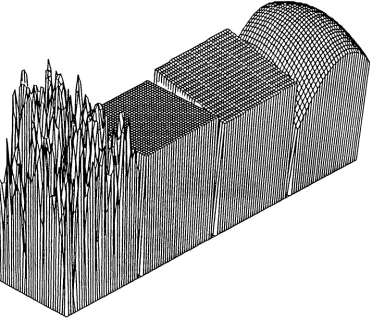
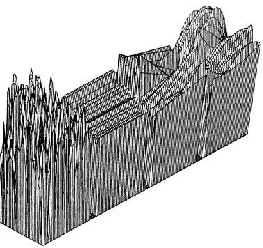
5.5. (a) Miss lJSA. (1)) Lena. (c) House. . . · · · . . . · . · · . · · . · · · · . · The segmented images using thJ1VD. (a) l\liss lTSA. (1)) Lena.. (c) House. ~)1 The segmeuted images using fila])' (a) Miss lJSA. (1))Lena. (c) House. ~):l

Comparison of the nonoverlap and overlap method. All image size and block size are 8 x 8 and -! x 4: respectively. . . 102 The class type images of l\Iiss {JSr\. (a) 0 percent overlap. (1)):j0 percent overlap. (c) 75 percent overlap. . . 106

1'}1e class t~"l)e images of Lena. (a) 0 percent overlap. (1)) 50 percent

overlap. (c) 75 percent overlap. . . ]08 The class t.~~l)eimages of House. (a) 0 percent overlap, (1)) 5U percent overlap, (c) 7!J percent overlap. . . 110 Modeling a. rough texture region using a. 2-D polynomial. From left. to to right are

the

3~ x 32 tree subimage ill Ilouse:

t.he

original"

t.he

zero-order model, the first-order 11lO(leI" and the second-order 1110del.. 120 Modeling a S11100th texture region using a 2-D polynomial. From leIt t.o to right are the 32x

:32

chill Sl11)i111age in Miss

trs

1\ : t.he original,

t.llp zero-order model. the first-order model. and the second-order 1110d{\1.121 Modeling a. rough texture region using a ]-1) polynomial. From k-It to to right. are the 32 x :l2 tree subimage ill House: the original, t.IH~ zero-order model, the first-order model, and

t

he second-order IllO(lt·~I.. 122 Modeling a. smooth texture region using a I-I) polyuomial. From

left

to to right are the 32 x 32 chin subimage ill Miss lJSA~ the original, the zero-order 1110(lel, the first-order 1110(lel" 811(1 the second-order 1110(1('1.1

:!:J

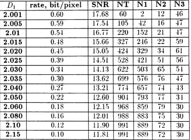
TIle decoded images of the test images with D]

=

2.0:1!j

an (I D2

=

2.:3G:3. (8) The decoded imageof l\Iiss

lTSA.

(1)) The decocled image of

J

Jf'lla.. (c) TIle decoded image of II ouse. . . 127 Plot of SNR versus rate, bit/pixel for Lena. D1 is variable a.B(1 !J'}. is

fixed

to

2.:36:3. . · · · · . · · . . . ..

1

~10

6.11 Plot of SNR versus rate .. bit/})ixf'l for House. D1 is variable and D'}. is fixed to 2.:36:3. . . .. 1·10 G.12 Plot of SNR versus rate .. lJit/!)ixel for House. D1 is fixed 2.0:3:) and L)l

is variable. . . 1~1 6.1:3 ']'he reconstructed images for Miss llSA. The images 011 t.het.op and

the bottom are coded at.1.0 lJit/l)ixe} with D1

=

2.UOl and

D

2

=

2.76

aucl 0.2 lJit./I)ixe} wit.h Dt = 2.00!)and

D

2 = 2.:36 respectively. . . 1J2 6.1! The reconstructed images for Lena.

The

images 011 the tOI) and the

1JOt.tOl11 are coded at 1.0 bit/})ixel with D1

=

2.005 and D2

=

2.71 and

0.2 bit/IJixel with

D1

=

2.050 and

D2

=

2.361 respectively. . . 1-1:3 6.15 The reconstructed images for House. The images on the 1.01) and the

bottom are coded at 1.0 bit/l>ixel with

D

1 = 2.U05 and

U

2

=

2.71 and

0.2 bit/l)ixel with Dt = 2.06 and D2 = 2.41 respectively. . . . lll 9.1 A crack code. (a) Set ,5': each point is labeled with a different lat.ter.

(b) Clockwise sequence of cracks around the border. beginning wit.h

the

crack At

at

t.lie 1.01>

of

A.

Tile

subscripts of t~1\b, I denote top, right ,

1)0t.

t.Ol11., and left" respectively. . . 156

List of Tables

5.1

Statistics of fractal dimension ill l\liss

lTSA

6i

5.2 Statistics of fractal dimension in Lena . . . Gi

5.:3 Statistics of fractal dimension ill House . . Gi

5.4 Fractal dimensions for each blocks, The column and 1"0\" index are ordered from the top left. The fractal dimension of each subirnage is given in table (a). Tile mean I' and the standard deviation (7 are given

in table

(b). . . ..

7:3

5.5 Fractal dimensions for each blocks. The coluuui and row index are ordered Iroin the top left. TIle fractal di mension of earII subimage is given ill table (a). The mean l' and the standard deviation (7 are given

ill table (1)). . . i-1 5.6 Fractal dimensions for each blocks. The column and 1"0\" index are

ordered from the top

left.

The

fractal

dimension of each subimage is given ill table (a). The mean I' and the standard deviation (7 are given

in table (1)). . . ..

i5

5.7 Fractal dimensions for each blocks, The COlUll11l and 1'0'" index are

ordered from t.he top left. The fractal dimension of each subimage is given illtable (a). The mean Ii and the standard deviation (7 are given

ill t.abIe (b). . . .. 7(.

5.8 Fractal dimeusions for each blocks, The COIUlll11 (\.11<.1 row index are ordered [rom the t.O}) left. The fractal dimension of each subimage is given in table (a).

TIle

mean Ii. and the standard deviation (7 are given

ill table (b). . . I I

5.9 Fractal dimensions for each blocks, The COlUl111l and row index are ordered from the tOI) left. The Iractal dimension of each su hi mage is given in table (a). The mean I' and the standard deviatiou

o

are given ill t.a ble (1)). . . .. 78

5.10 5.11 5.12 5.1

:3

5.14 5.15 6.1 c ') u.z 6.:3 G.-! 6.5 6.6

G.I

6.8

G.9

6.10

s.u

G.12

Fractal dimensions for each blocks. The column and 1'0"· index are ordered Irom the top left. The Iract al dimension of each su bimage is given in ta1)le (a). The mean II and the standard deviation (j are given

ill table (b) " " . " .

Fractal dimensions for each blocks. The COI\111111 and row index are ordered from t.he top left. 1'11efract-al dimension of each subiuiagr is given ill t.able (a). Tile mean JI 0.11<.1 the standard deviation a are given ill table (b). . . . Fractal dimensions for each blocks. TIre column and row index are orclered from the tOI) left. The fractal dimension of each subimage is given ill table (a). TIle mean I' and the standard deviation a are given ill table (1»). . . " . . . .

The number of segments for test images using

t

h

con

=

5.5.

The number of segments for test images using

t

hJ

r:

D.

The 11umber of segments for test images using t

hap.

Pixel percentage of each class in l\Iiss

l.TSA

Pixel percentageof each class

ill

Lena . . . Pixel percentageof each class ill House . .

Pr-rcent.age of the pixels in each class ill Miss lTSA wit.h 50(A'. overlap. 1)1 variable .. and D2

=

2.:3(;::1. . . · . . . · · · . . . .

Percentage of t.he pixels in each class ill l\liss lTSA with 50(/(, overlap, D_t

=

2.0:3,) .. and D2 variable, · . · . · · . · · · . · . Percentage of the pixels ill each class in Lena with 50(;(, overlap .. D1

variable .. and

D'2

=

2.3G:_J. · · · .. · .

Percentage of the pixels in each class type in Lena with !jO(j{, overlap ..

D

I

=

2.0:J5 .. 0.11(1

D'2

variable. · . · . · · · · . . . . · . . · . . · · . . .

Pcrceutage of the pixels in each class ill House with !jO~1 overlap .. D1 variable. and J)2

=

2.:jG3. · · · . . · · . . · . · . . · . · · · . Percentageof the pixels illeach class ill House with 50(/(\ overlap ..

D

1

=

2.0:3,) .. aucl

D'2

variable. . . · · . . . · . . · · · . · · . · · . . . Summary of the numbers of the total segments and the boundary points

using

D

₁

=

2.0:3·5 and

D2

=

2.:363. · · . · · · . . . · . · . · . . · · · .

SU111111ar~· of hits to represent the boundarv using the three (lifrerent. cocliug. . · . . · . . . · . . . . Sunnnarv of the numbers of the total segments and the l>erct'i,oed ("011-staut regions using D1

=

2.0:35 and D2

=

2.::16:3. . .

Summary of the number of bits to represent tlie const-ant, rpgioll .

x

80

81 8~J

lOG

IO~ 110 112 112 112

II!)

II

!j j Ii

6.1! The SUI11 of squared error (SSE) values for each model. 120 G.1!) The SUl1l of squared error (SSE) values for each 1110d('1. l~l

G.16 The sum of squared error (SSE) values for each 1110<.1(:'1. 122

(j.lT The sum of squared error (SSE) values for each model. 1~:J

(i.18

S

11111111ary of the 1111)nlx-rs of t.he segmen t.s ill the smooth and rougl1

textural regions and the number of bits to represent those regions using a 1-D polvnomial, '!'he polynomial coefficients were encoded using the arit.luuetic code. . . 12-1

6.19 Summarv of coding

information ill

l\Jiss

lfSA.

D1

is

variable and })2

is

fixed to 2.:36:3 0 0 • • • • • • • • • • • • • J:31 6.20 Summary ofcoding information ill Lena. D1 is variable 0.11(1

D'),

is fixed

to 2.:JG:J. . . .. 132 6.21 Summarv of codiug information in House,

D

1 is variable and

D'2

is

fixed to 2.:363. . . 1:3:J

6.22 Sunnnaryofcoding infonnatiou ill l\liss lJSA. D1 is fixed to 2.0:3!jand

D2 is variable. . . J:JJ

6.2:3 SUl1111)Clry' of coding information ill Lena. D₁ is fixed to 2.U:j!j and D₂

is variable. . . J:3!j G.24 Sununarv of coding information ill House. D₁ is fixed to 2.0:35 and

D'2

is variable. . . 0 • • • • • • • • • • • • • • • • • • • • • • • 1:3G 6.25 S1l111111a.r~·of coding iuformat.ion in l\Iiss lTSA. D1

=

2.0:l!j~ D2

=

2.:lf;:3'1

7'11f31'2 = 60 and

T

11t;Tl is variable. where

T II

_{f3 1}o. and

T

lIEl''), are t.he thresholds of regions beloiugiug to the Sl1100th and the rough textures respectively. . · · · · . . . 1:37 6.26 Summary of coding information ill Lena. D1

=

2.0:j!j~ D2

=

2.:3G:J~

T11e1'2

=

GO 01](1 T Helo] is variable. . . . .. 1:37 G.27 SU111111Clf3· of coding information ill Ilouse, D₁ = 2.0:3.)'1

D'2

=

2.:lG:3~

1'//'31'2

=

liO and

T lIt:

r1 is variable. . . 1:38 6.28 Summaryof coding information in Miss (TS.lt\.

D

1

=

2.U:3.'j~

D'2

=

2.:3():J~

]'Hf 1· ]

=

25 and 1'1Ie1'2 is variable, . . . 1:38

G.2~) Suuunary of coding information ill Lena. D₁ = 2.0:35, D

2 = 2.:3G:3"

]'Hf l · ]

=

25 0.11([ 1'j 1f. 1·2is variable. . . 1:3U

G.:30 Summary of coding information in House. D1 = 2.0:35" D2 = 2.:3G:J"

1'Hf3 1·]

=

25 and TIIf3T2 is variable.. · . . . 1:3~)

1

Introduction

The (ligital representation of an image requires a verv large number of bits. For

example, a

·512

x

512

pixel,

25G

gray level image requires over two million

bits,

This

large number of bits is a. substantial drawback when it is necessary to store or transmit a, digital image, Prior to transmission or storage" one would like to have a svstcm

that reduces 1.11is number as 11111Cl1 as possible. while keeping the degraclation ill th« decoded image to a minimum. This is tile goal of image compression, often referred

to as image coding.

EaTI,"

efforts ill image compression, solelv guided 1)~· inlonuation theorv, led

t.o

a plethora of methods, TIle compression ratio" st.art.iug at one with t.hefirst digital picture ill the early 1960"s" a ppeared to have reached a saturation level around 10:1

ill

the early 1980"s. This, however.

(lid

not mean

that

the upper bound given bv

t.hp

entropy of the source had also been reached, First." this entropy is not known aud

depends heavily on

t

he 1110(lel used for the source" i.e... the cligital image. Second, informatiou thcory does 110t. take into account

what

the human eye sees and 1I0\r it. Sf'es. Receut lv. techniques attempting to overcome these limit at ions are incorporat iug

properties of the human visual system (JI\~S)ancl tools of image analysis

into

image

compression t.o

achieve high

compression ratios with small loss in visual qualitv, This

reasoning follows Irom t.he fact that ill many compression applirat ions __ a human is the final observer of the image opera t.ed u1>011. A pplica t.ions of yo rious 1110d(,Is of tile II\rs have ill fact been empiricallv found to i11IprOYC compression performance [2!j~ -13 __ 57, 71~ 83].

One such technique is segmentation-based image compression [7~ 3n~ -l;3~ 7

J].

In segmentation-based image compression. the image to be compressed is segmented,

i.e. the pixels ill tile image are separated into mutually exclusive spatial regions

based 011 somecriteria. Once the image has been segmented, information is extracted

describing the boundaries (shapes] and textures [interiors] oftheimage segment s __and

compression is acllieved by efficiently encoding this informat.iou. Unfortuuatelv,

t

here a re Iimi t.at.ions wit.h segment at.ion-based image compression. The main limi t.a

t

ion is

due to the fact that the image (lata have been segmented into regions of constant

intensity. III complicated texture areas __ a good representation of the texture requires

manysmall segments, However, ill order to get

10\'"

bit rates, the numberofsegments must l)e limited and thus the quality is degraded.

We overcome the texture representation problem ill the research described ill this report 1)j9 proposing a methodology for segmenting all image into texturally

homoge-neous regions with respect to the degree of roughness as perceived l)y t.lie

I-I\9S.

The

segmented image information is then encoded for transmission. The proposed

algo-rithm is applied to three different t.ypes of imagery. The first is a head and shoulder image with lit.tle texture variation. This image is typical of video teleconferencing applications and one which the previously proposed segment.at ion-based compression

techniques are best suited. TIle second is a complex image

with

mauv edges and

t.he third is a natural outdoor image with

highly

textured areas. The previous

pro-posed segmeut.ation-based compression techniques (10 110t. 'York well for the' second

and third images. However. the proposed texture-based image compression t.echnique

works well for not only the first but also the second and the third t.\"l)(' of image.

III

tlie proposed texture-based image compressionalgorit lun. t.heIract al dimr-usiou ..

t.IH~ expected value .. and t.hejust noticea bledifference (.JND) are the measures used to characterize the texture information. The measured quant.ities are incorporated iut.o a c~llt.roid-Jillkage region growing algorithm [:32]

which

is

used to segment

each

image iuto three texture classes. The region growing algorithm is directed l)y the texture

feat.ure distance l)pt,,,eell image blocks. After segment.ation .. the image can be viewed

as being C0111])Osecl of region boundaries 0.11(1 texturallv homogeneous regions. Since the decoded images will be viewed by humans, our prime motivation is the production

ratios.

The second aspect of LItis work is to propose appropriate compression t.echniques

for the three textural classes 0.11([ the region boundaries, The three classes, I.. IJ~ and

A binary map representing the boundaries of the regions is encoded using a 1110di-Iiecl aclapt ive arit.lunet.ic coder [G2 .. 7:3.

To].

III

our work .. the represeut.ation of thp bounclarv information using blocks .. Bot pixels .. provides us with higher compression. Regions which belong to class I are modeled as flat planes .. hence tllf'y onlv need to have their mean intensity value transmitted. The means are then encoded using a modified adaptivearithmeticcode, TIle highest compression ratio is achieved for class I. Because of the sensitivity of the I-I\··S to 111j(1<.1Ie range spat

ial

frequencies .. regions belonging t.o class II require a 1110re accurate representation. Regions lx-longiug t.o class III contain the highest spatial frequencies. The II\.TS is less sensitive to thc high

spal.ia] frequencies .. thus these regions call be more highly compressed.

The

texttire

information in class II and III are modeled bv polynomial Iunctions. Higher COI1)-pression is achieved for class III bv allowing theerror between t.lieoriginal image and the modek-d image to be greater tl1a11 for class II. The result. is a segmeutation-based image coding system

wit.li

high compression and a s111al110ss in visual quality.

In SU111111ary, the main cont.ributious of this report are:

• a new technique for segmenting an imageinto text.urally consistent regions: • use of the fractal dimension for relating the SI)at.ial freqHeney of t.ext.ures t.o

the spatial frequency response of the human visual system:

• a new algorithm for encoding the segmented image information: and

• good quality compressed images at. 0.2 to 0.-1 1)1>1) for higher text.ural images.

In Chapter 2, the prerequisite background material. emphasizing "York which is pertineut to t.lie methods used ill this research is covered, as are the properties of

the II\rs.

III Chapter

3.,

fractal models ill texture analvsis are covered.

The

fractal dimension and t.lie power spectral density (PSD) of the fractional Brownian fuuct.iou

(I~}3F) are clerived 0.11(1 discussed. III Cha pt.er 4 _a complete description of tlu- new image compression system is given. III Chapter 5~ image segrnent.at.ion is developed

and evaluated using properties of the II\?S and the fractal dimension. III Chapter ()~ t.IH:~ mixed coding scheme is described and the performance of

t.hp

new image

2

An Overview of Image

Corrrpr-esaiori

2 .1

Introduction

Manv dat.a processing applications involve storage of large volumes of dot-a. For

ex-ample, t.orepresent a 512 x 512 pixel,25Ggray level digi t.al image.OYf')"t.wo luilliou bits

are required. IIIaddit ion, the number of data processing applications such as ill t.IIP

areas of meteorology, military reconnaissance, medicine, and electronic publishing is

increasing rapicllv. At the same time .. there has been a proliferationof computer com-municat ion net works and teleprocessing applications .. which ill '·0]ve massive transfers

of dat.a over long-distance communication links. For example .. to transmit all uucom-pressed 512 y 512 pixel, 256 gra~·level digital image over a G-!l\hit/s channel requires more

t

han t.hirty seconds.

TIle

requirements aTP even higher for a color image of

the Sa.IIICsize. To reduce

t

he (lata storage requirements and the (lata conunuuicat.iou

costs. there is a llPpd to reduce

the

redundancyill the data representat.iou. Image

corn-pression techniques have attempted t.oreduce the amount of data needed 1.0 transmit or store digital images .. while keeping the degradation in the quality of tlie decoded

image to a minimum.

III this chapter, we

briefly

review the recent advances ill image compression tech-uiques.

III

general. any imagecompression method call be broadly classified as lJt\ing

ei t.her statist icallv- based (algebraic] or symbolicallv- based [st ructural). The st.a

t.is-tical approaches to image compression are based on informatiou

t

hr-orctic principles

aud the met110dsused usually involve verv localized. pixel-oriented ff'at ures oftho

im-age. A sununarv of these techniques is presented ill Section 2.2. However. due to t.he

limitations of t.he st.at.ist.ical approaches. researchers were interested in finding a new approach t.o image compression for very

10,Y

bit rate applications, Many of the

11e,,-approaches are known as symbolically-basecl (second generation [.1:3]) image

C01l11>)"PS-sion. Syinbolicallv-based imagecompression methods employ tools of image analysis and properties of the human visual system (11\7'S) to achieve good image quality at.

verv low data rates. III symbolically-based compression, the geomet.ric structure of

t.IH~ image scene is emphasized, as opposed to tile algebraic structure of the pixels used bv statistically-based compression methods.

III

Section 2.:3 we sununarize t.he

work in the developing area ofsymbolically-based image compression.

Image compression methods can be further classified beyond t.he two main

cate-gories mentioned above. For example, theclassificationcan be based011 the techniques

t.he compression method employs and the distortion the compression 111eth()(1

iut.ro-duces ill the image. One possible classification of compression methods is as adaptive

or non-aclaptive. In a typical image, the stat.ist.ical characteristics of all image differ

considerablv Iroin one region to another. For example, walls and skies have

approx-imatr-lv uniform background intensities, whereas fa.ces and trees have large, dot.ailed

variations in intensifies. To compensate for this. parameters of the coder are adapted

to variations ill thelocal statistics ofthe image. such as local image contrast .

.4\

coder

that employs such parameter variation techniquesis classified as adaptive. If t.hist.Yl)P of variat ion is not used, the compression technique is non-adaptive. Some examples

of adaptive image compression techniques are adapt ive clillerent.ial pulse code

lation , aclapiive delta modulation. and adaptive transform compression

[:n.

28.90].

Auot.lierclassificatiou describes whet her themethod is distortionlessor non dist

or-tionless, If a compression method is dist.ortionless then the decoded image is perfect recreat ion of the original image. Nearlv all distort.ionless techniques are based 011 information theoretic approaches and usuallv attain data rates in the neighborhood

of two or lour bits })pr pixel (1)1)})) for an original 8 bpp image [-10]. Non-distortionless

compression methods introduce differences between the decoded image and t.he orig-inal image .. but they allow lower (lata rates. However .. the decoded image IllUS{. bp

kept as close to tile original as possi ble.

techniques.

2.2

Statistically-Based

Image Compression Techniques

l\lost of the compression techniques developed from the early 1~)60"s to t.hepresent

fit

into t.he category of the statisticallv-basecl image compression techniques, 1\block cliagraui of tIle gr-ueral st.atist.ical image compression svstern is shown in Figure 2.J.

']'IJe st.atist.icallv-basecl image compression techniques address t.lieimage compression problem Irom all information theory viewpoint, with the focus 0]1 eliminatiug

t

ltp st.at.ist.ical redundancy among the pixels in the image.

IdeaII,\".. the 1110st useful preprocessor... as shown ill Figure 2.1 .. is a t.ransformat.ion

of the image to the most suitable domain for coding. The best one ran do is find a pre-processor that l11a})S the (lata into uncorrelat ed spat ial-domain data or a s('t. of independent transform-domain coefficients. For example. the

mapping might

rp1l10YP

(

Decoder

-

Preprocessor

:- _Encoder t o

-(Decorrelator)

-

Channel) :::

-

-Image or

Sequence

of images

Reconstructed image or

Sequence of images

Figure 2.1: A general statistically-basecl image compression system

the mutual redundancy between successive pixels or take the discrete Fourier

trans-form of the image pixels, TIle desire for the pixels to l)e iudependeut is based on

rate-distortion theory. Hate distort.ion theory defines t.heoptimum coder to he the coder that attains the best possible signal ficlelity for a given elate rate, or t.hecoder that attains the best possible (lata for a given signal ficlelity [26].

coding blocks of (lata" rather than individual (lata points, III fact"

t.he

optimal coder is achieved as 1\7 ~ 00" where l\T is the length of the block of (lata being coded [81].

All

exampleof such a block coder is a vector quant.izer [26]. Obviously.. a coder wit.h infinite block Ieugth is impossible, and even a coder wit.h a reasonably long block

length is difficult to design and implement. IIo''''C'Yf'l\ it bas l)pel) shown that l\~ coders of block leugth one are nearly as good as (withill about O.~!j l)it.s/salll}'](') (is 011(' coder of block length ]\i" for the squared error distort ion measure [3:1]. Th us"

jf

t.he dat.a SC\.111IJles call l)e transformed so that

t

hev are statistically indepeudcnt , 1.11<'11

nearly optimum coder performance can l)e achieved with a coder of length one, i.c. a simple quant.izer. This fact forms the basis for st.at.isiically-based image coding.

Manv excellent reviews of st.atistical image compression techniques exist in 1lie

lit.erat.ure. III 19G6~ Schreiber wrote all interesting review of the early vears ofimage

compression [79]. Pratt [67] presented all overall sununaryof the state of image C0111-pression ill 1979. Net.ravali

and

Limb wrote an informative review

of

image COllI pres-sion techniques ill 1980 [56]. as did Jain ill 1981 [:36].

III

addition ..Jain [:36] contains an extensive bibliography of publications ill image compression and related areas. 1\1usmann, et al.

[!J-l]

presented a review

of

t.he advances made ill image compression techniquessince 1981'1 with specialemphasis placed on advances in thecoding of color television and video-conference signals. III addition to these review papers, there arc

many books and special issues of professional journals which deal exclusively with i111age compression [l~). 20. 29., 80].

III general. statistically-based image compression techniques can be categorized into five classes: predictive coding, transform coding .. hybrid coding. iut.erpolalive

and extrapolative coding, and a miscellaneous category [,5G].

Predictive image compression operates directly on the pixel intensitv values ill all image, The objective is to generate cUI error signal bv subtracting a predicted pixel value Irom

t.IIE'

actual pixel value. TIle predicted pixel value is a weightpd average

(Cl(IClI)t ive or nonadaptive] of spat.iallv and/or temporally adjacent pixels, The only

information

that

neetls to be transmitted is the error signal.

Transform image compression 111allSall image into a domain whore a large amount

l Ivbrid coding refers to methods which utilize a combiuation of pr--clictive and

translorm domain information. Predict ive and trausforrn coding techniqueseach have

some att ract ive characteristics aud Iimilat.ious. The combination of these two

tech-niqueslias thecapabilityof achieving higher COI11})ressio11than either of the t.wo coders

individually and has t.headvantages of hardware simplicitv of predictive coders and

high performance of transform coders. For more details" see [:36., !j1" !j(L ;5].

Interpolative and extrapolative methodsextract a subset of the pixels in all image 1)~' subsampliug. This subset is then transmitted .. and the decoder interpolates or

extrapolates to fill ill the missing pixels.

TIle

subsamplingof the image is done ill

the

spatial and/or temporaldomains. Simple interpolative coding consistsof the

following

steps: 1) choose certain pixels for transmission, 2) construct an iuterpolation of t.he nont.ransmit.ted pixels, all<.1 :3) evaluate the interpolation error. The interpolation

function can be zero .. first-order, or higher order 1)01~"110Illials. It has been shown

that interpolation using straight lines is quite effective a11(1 not much is gained by illterpola tion using polynomials of higher degree

[i).

If higher orcler 1)01~·110111ia.l8are

used in the interpolation, it may l)e necessary to transmit polynomial coefficients .. and the subset. of image pixels. In addition .. the computation t.ime involved in the

intr-rpolat.ion process grows rapidly with the degree of the fit.ting polynomial. For 1110re det-ails. see papers [15" 21., 45" 55].

Examples of some important st.at.ist.ically-based techniques t.hat <10 not.

fit.

into

any of tlie a bove categories include bit-plane coding .. curve fitting methods, and

run-length coding[21" 31]. Someof these methods aresimplyone-dimensionalcompression methods applied to two-dimensional image signals,

Symbolic description oftheimage ("message")

(Channel) Decoder

- Symbol

,

Encoder

~

-

-Extractor

::

-

:::.

Image or

Sequence

of images

ReconstlUcted

image or

Sequence

of images

Figure 2.2: A general symbolicallv-based image compression svstem.

2.3

Symbolically-Based Image Compression Techniques

The st.atist.icallv-based image compression techniques .. solelv guided bv iuforruatiou theorv.. led t.o a plethora of methods, The compression ratio appeared 1.0 have reached

bit rates were desirable. A 11e,Y approach t.oimage compression was necessarv ifhigh

known as symbolically-based or second generation image compression t.eclmiques. A

1)10ckdiagram of a general S~·1111>olicimage compression system is 8ho',"11 ill Figure2.2

There are t,YO main limit.at.ions ill the

st.at.ist

icallv-based image compression

tech-uiques.

First ..

since the entropy of the digit al image is normally not known .. t.h~

upper bound based on an estimate of first-order eutropy cannot. 1)~ expect.ed to work

'Yell. SeCOll(1.. information theorv does not take into account

what

a human. 111P

final observer of the image informa

t

ion. sees and

110'" it

sees. S~·lllbolically-based

im-age compression techniques have <lttellll>tf.'d to overcome these limitations corubiuing properties of the II\~Sand tools of image analysis to get high compression ratios with small loss ill visual quality, Global, rather than local pixel-oriented Ieat.ures of the image are emphasized. Examples of such glolJal feat tires include the size" shape. or

orientation of objects ill the image scene. Extracting the tvpes of features t.hat can

l)e used to provide a symbolic description of the image scene is t.he ultimate goal

of the message extractor ill a symbolic image compression scheme. This symbolic description might take tile form of a list of scene at.tributes. for example "there is a

chair ill the ul>j)er left corner of the scene ." or ""1110.11 ill a reel shirt is running from left. to right ill the scene while turning his head and looking at the camera." Notice

t.hat these are high level descriptions of the scene and (10 not (leal with actual image pixel values, but with the scene content, The encoder then efficicnt.lyencodes

t

hese scelle descriptious or "messages"'! •

Since the symbolically-based image compression techniques are Iairlv new _ there havenot l)pell many general reviews ofthese typesof compressionmethods published

vet. There are" however, several review papers of the second geueration compression

techniques ill the literature [-1:3]. III addition to this paper, there is mention of some

second generation compression techniques ill [!j4,5G].

1'0

better appreciate the symbolically-based imagecompression techniques, the

l"f']-evant propertiesofthe

H\'S

are first described

ill this

sect.ion. Following

t.hat

is (t

dis-cussion of the majorsyrnbolicallv-based image compression t.t:'ClllljqtleS~pyramidal im-age compression [9]" directional decomposition-based compression [-13]" segment.at ion-based compression [7" 38], and Iractal-based compression

[!)'l

35" 89].

2.3.1

Tile

H'urnan Visual Syst.em (HVS)

III

mauy applications like video phone, teleconferencing. T\·. and medical imaging,

the final ubser,-er of the image data is a human. Thus it is very important t hat. all image coder ]Je desigued to meet the needs of t.hehuman observer. Ideallv, no bits should ]Je required to encode the information ill all image t.hat is not important to

the 111l111o.Il viewer and all the bits should be used to encode the iuformation that. is important to human perception, For this reaSOII., the 1110re that is known about. t.he requirements of the IJ\·rs" the l>E~tterthe coding method can be designed. However. the II\'~S is very complex and not completely understood. therefore, making image coding a difficult problem.

Despite the complexity of the II\,rS., a great (leal of research has been done in all effort to determine some of its basic properties. This research is generally based 011 experiments with human subjects, so the results are necessarily subjective.

Dis-cussions of some of t.he basic techniques and significant results ill the area of

II\·TS

research can lJe{OtIIlClill [43" ,56~ 79]. TIle books by Cornsweet [1-1] and Marr [52] are useful references on human vision. Here we will briefly suuunarize some of t.he 1)108t.

well established properties of the ll\rs [7f)] for image coding applicat.ions.

A property of

the

]1\'S

that

has been studied extensively is contrast seusitivitv, Contrast sensitivity is measured

by

showing a subject a test pattern. and varviug

the

1+ ~I

I

~I

I

50 100 ISO 200 I

(a) (b)

Figure 2.3: A simple contrast seusit.ivity measurement

function of I ill Figure 2.:3b.

Figure 2.:31) sI10\,"s that the JJ\iS has greatly reduced contrast sensitivity in verv bright or verv dark intensitv regions of all image. However, this experiment is

time-consuming. All alternative is a 111etl10d introduced by Hamilton [:30]. It. is referred t.o

as a split-field technique, measures the .JND quickly and reliably. Here. t.he display is divided clown the middle into two equal-size fields, see Figure 2.-1. The

left

11('1<1 is a constant intensity reference field and the right. field begins

at

the t.Ol)

wit.h

the

reference intensity and increases linearly til) to -10 steps above the reIcreucewit.heach

lCY('1

presented as a baud 20 pixels in height To perform the test" an obse-rver simplv

Figure 2.4: Perspective drawing of the split-field experiment

The contrast sensitivity of a human call be used for designing quant.izers, as a

threshold for the split-merge condition ill segmentation-based compression. or for

human vision based image distortion measurements, More discussion of t.he use of this technique and how we incorporate .JND measurements into

t.he

proposed codec

will be given ill Section 5.~1.

A second important property of the

II\lS

is the modulat.ion transfer Iuuct.ion (l\ITF). TIle l\ITF is the response measured l)y all observer who was shown t.,YO SiIU:' wave grating transparencies, a reference grating of const.aut contrast and spat.ial frequency, and a variable-contrast test grating whose spatial frequency is set at. some

value different from that of the reference [66]. The contrast of the test grating is

varied until the brightness of

t.11E'

bright and (lark regions of

t

he t.wo transparencies

a-j)J)f.'ar ident.ical, TIle typical curve of the M'I'F is ShO'YII ill Figure 2..1.

TIle shape of the :t\ITF curve is

similar

to a

baud-pass

filter and suggests

that

Contrast sensitivity (DB)

50

40

30

20

10

0.5 1 5 10 50

Spatial frequency, cycles/degree

high spatial frequencies. This implies that the middle spatial frequencies plav a more

import.aut role in perceived image quality than other frequencies. This proportv

is verv important ill segmentation-based image compression [38]. For eXc1.1111>le"

if

all image is segmented into regions with respect to

t.he

information content. at. the

different frequencies. the image coder should require 1110re bits 1.0 encode regions

which contain 11li<I<.1Ie spatial Irequeucies to maintain quality, a)1<.1 USf' very Iew bits to encode regions which contain

10,'"

and high frequencies which the I-I\·l'S is less sensitive t.o.

A third propert y of the lI\"S is saturation effect. The contrast sensit.i vitv of the eve is known to decrease as t he intensitv of the visual st.imulus 1110YPS aw av from the middle range of intensitv yalues

[1.1].

That is, the Pyf' bas reduced sensit.ivit.v

to differences at very

high

gra~· levels and differences at verv low gray levels. This l)hellOlllenOll call be used t.o reduce the dynamic range of the image data.

Each of the a bove properties hell) to characterize the aspects of the II \rs tliat are 1110St important in the development of image compression techniques. \\:e now proceed to present l.he syiubolically-based image compression techniques.

2.3.2

Pyr-amidal

Irnage Compression

Pyramidal image compression

[9]

features a hierarchical representation Ior t.he

im-age. The hierarchical structure is similar to that of the nervous system and it. uses functions similar to those ill the II\:'S. The representation is geuerated using all it.-erat

i'''e

applicatiou of 10\"'-I>a88 filtering. A block diagram of this system is shown ill figure 2.6.

Starting

wit

h the original image ~r(11l'l11)'1 a low-pass version ~rl(1H'\11) is

COll1-j>uted using local averaging with a unimodal Gaussian-Iike two-dimensional impulse response. The 10\\"-}Jas8 image, wit.h a cutoff Irequeucy of .fl'\call be Yie'\,,(:lc.1 (\S a

pre-cliction of~r(111"'11). Tileprediction error (1(171"11) is the difference between t.heoriginal

image and tlre low-pass filtered image.

(2.1 )

<-'learlv. ifone coded the10'\,,-1)o.S8 imageand the prediction error this would he equi v-alent t.o directlv coding the original image. Compression call be (\('hie\"ed

wit.h

this

rf'])reSellt.atio11 ill two wavs: (1) Since the error image is high-pass and t.he II\'S has

Gaussian Planes

Laplacian Planes

Quantization Reconstructed

Laplacian

Reconstructed Gaussian

x (m.n)

n

x (m.n) 0-1

xj.m,n)

Original

Image

e (m.n)

n+l

I

•

I

'II

Reconstructed

Image

Figure 2.6: Block diagram of the pyramid coding method

}PSS seusit.ivitv at. high frequencies .. the error image call be coded

wit.li

Iewer bits tlian tlie original image, (2) B~· the two-dimensional sampling theorem. tile iO\Y-IJaSS filtered image call l)e represented with fewer samples

than

the original image.

An advantage of pvramidal coding is that the procedure described above call be al)})lie<l iteratively. S})ecificaJl~:,.. the low-pass filtered image ~rl(111.. 11) call he filtered a second t.ime, at a lower cu t-off frequency .(2 (tvpicallv

half

the Irequr-ncv of tlie first. filt.erillg operat.ion ), This twire-filtered image ~r2(111 .. 11) is now a prediction for ~l'1 (111 ..11 ) ..and the error for this predict ion is

(2.2 )

After n iterations .. a series of prediction error images fl (111 ..11)., ... .,f_n(111., 11) are 01)-t.ainecl. If these images are viewed as stacked one above the other. the result. is a. pyramidal (lata structure. At each iteration the dimension of the error image is

rpdllcpd (t.hrongh spatial decimat ion) 1))7a factor equal t.o t.h~ ratio of t.he cutoff

frp-(lUPJICies used ill that iteration aucl the previous iteration (t.ypically a factor of t.wo).

The resultiug error images are quant.ized(\.11(1 transmi

t

t.e(l to t.herecei ver.

1"'0 reconstruct tlie received image data... int.erpolat.iou filters are used to

recon-st.ruct tlu.l ('1'1'01' images from their decimated versions. A pixel-by-pixel sum of the reconstructf~d error images vields the decoded image . A nice Ica t.ure of this svstcui is

t.hat the quality of tlie decoded picture can l)e improved as desired at. the expense of a lower compression ratio. Good quality images call be obtained around 0.8 bpp.

2.3.3

Dir-ect.ional Decornposit.ion Based Image Compression

1~he molivation of directional clecomposi tiou image compression

[43]

is largelv d ue to

t

he existence of direct.ionallv-sensitive neurons ill the

H\rs.

In this met.hod. the orig-inal image is decomposed into a series of images using filtering operations emploving C;allssiall windows. TIle entire spatial frequency plane is covered with one ]O\Y-])ClSS filter .. plus a set of high-pass, directional filters.

TIle

purpose of

each

directional filt.~r

is to extract edges ill the image witli a particular spatial orientation. The filtered

versions of the original image are coded to Iorm t.he compressed image.

The lllessnges to be coded are t.he low-pass image and the direct.ionally-filt.ered

images. The low-frequency component is suitable for t.ransforrn coding. Each of the directionallv-filterecl images isspatiallydecimatedand then represented bv coding the positions ancl magnitudes of the edges in the decimated image. The edge posi

t

iOIlS are coded using a run-length II ullman codeI! a.11(1

t

11e magni

t

udes of

t.he

edges are quantized and coded using 3 bit coclewords. This coarse quantization is possible due

to tile reduced contrast sensitivity of the II\.!S at high frequencies.

1'0 reconstruct the original image, the low-Frequency component is obt ained bv

inverse transforrniug the coded coefficients and then the high-frequeucy dircctioual

edge images are reconstructed l)~r decoding the edge information and int.erpolating.

Once all t.he filtered images have been reconstructed,

they

are summed to Iorrn the final decoded image. This method call achievecompression ratios around 0.2 to

o.!)

1)})}>.

2.3.4 Segrnentation-Based Image Compr-ession

For segmentation-based image compression techniques [7.. 38]I! the image to l)e

com-pressed is first. segmented. In image segmentation. the pixels ill all image are divided

iJJ1.0 lllllt ually exclusi ve spatial regions based 011 some cril.erin. A It.eruat.iYP].'YI!

tilt.)

cri-t.eria used could 1)e as simple as the similarity of the pixel gray leyels (yielding flat image segments]

[12.. 72].

TIle

criteria could l)e 1110recomplex, such as how

'Yell

the pixels

fit

a given planar model (facet-based segment.at.ion ) [80]I! a twe-dimensional 1)01~·110111ialll10<.lel[i]I!

a

statist.ical

model (texture-based

segmentation] [6U~

821! 88]

or a fractal 1110(lel [:38 ..

G3].

Properties of t.he

II\tS

can

also

be incorporated iut.o

t.he

t.eria to obtain a reconstructed image with a small visual loss, For example, contrast sensitivity and the l\ITF, call be combined with classical segmcut.atiou algorithms. In general. seglllE'lltat.ion is carried out. in three steps: preprocessing. region growing.

and elimination of artifacts.

Thepurpose ofthe preprocessing is to reduce the local grallularit~·of original image ,vit.liout affect iug its contours, so that very small-sized regions are not. obtained after region growing.

A key

problem in preprocessing is the reconciliation of1.'''0 apparcntlv

cont.radir torv goals; namely. granularity removal and edge preservation. Most of t.he gra-lItllarit~o removal filters have low-pass characteristics an <.1 therefore smooth the edges as well, Au inverse gradient filter [86] may be a solution of the problem. This Iilt.er behaveslikes a 10\"'-I>as8 filter ill areas free of contours a11(1 like all all-pass filter ill

highly

contrasted areas.

TIle mechanism of region growing is the following. Regions to be extracted must be characterized with some property ill the first step, Tile property might be, for example, the gra~olevel of a pixel, the variation of t.lie grav level, or t.he energy within a given frequency l)a11(1. The selection of this propertY plays a verv i1111)01't.allt. role

ill

t

he complexity of the method and ill the exactness of tile contours obtained after segmentation. Then. starting with a given pixels ill the picture, its

ueighboring

pixels are examiued t.o see whetherthey share the same property. If this is the rase .. the pixel is included ill the region, and ill turn, its neighboring pixels are examined, aud so OIL

'''''Ilell there are 110 1110repixels left." COIlnected t.o the region and sharing thf-l same property.. t.lie procedure stops and restarts at any other pixel which is not. includr-d

ill

the first region. The segmentation is complete when all

t.he

pixels of th« picture are assigned to some region. The above procedure call also {\})l)ly to the block-based region growing algorithm if a feat ure set. based 011 blocks of all image is defined.

Alter region growing. there are artifacts such as false contours, which do not. correspond to real objects in the original image. such as 8111all regions gCllel'Clt.cd bv

noise. The nU1111)er of these contours is much higher than that. of the objects ill t

hp

original image. Two \Ya~9S are available to remove t.his problem: oliminat.icn of t.li« small regions and merging weakly contrasted adjacent regions. If it is assumed that

regions coutaiuing a number of pixels less than a threshold are llot siguilicant.. their elimination drast.ically decreases the number of s111al1 regions. To avoid t.he creation of holes in t.heimage, these regions are included in one of their adjacent regions. 1'0 minimize the corresponding distortion, the enclosing region is chosen as the adjacent region whose mean graj· level is closest to that of the 8111a11 region to be included. The second possibility to decrease the numberof regions is to merge adjacent regions

whose contrast is below a. certain level. The contrast between adjacent regions IS defined as the mean gray level difference calculated along their C0I11111011 border.

After the segmentation is COI111)J~t.e'l t.heimage consists of a set of disjoint. regions separated bv contours, Both the contour (boundary] iuformation and

t

he region

inlormat ion must 1)E' encoded. The contours may be approxunated with straight lines and circle segments and then the information describing this approximation is

encoded [·13]'1 Alternatively. a biuary image describing where segment contours are

located ill t.he image may be encoded [72]. The interior of a segment is represented by encoding. for example. tile coefficients ill a polynomial models describing PRell seguient, or for flat segments, the average gray level of the pixels in each segment.

Kuut ..

ct

al. [-1:3] divided an image into segments using a region growing technique based on informationofintensityvalue, Contour coding is carriedout

ill

a three-mode

procedure: 1) approximation bv line segments, 2) approximatiou 1)~· circle segments,

and 3) without approximation. The cost, associated wit.h each 1110dp'l ill terms of

nurnber of bits for coding, is evaluated and the cheapest 1110(1(:' is chosen. Texture

coding is used to encode the missing part. of tlie messages with a t.,Yo-dinl~llsiollaJ polynomial Iunct.ion. All underlving assumpt.ion is that within each region t.here is 110 longer any sharp discont.inuit.v.

Tile

order of t.he polynomial is detcnuiIHld as a Iuuct.ion of

t

he approximation error and of the cost involved ill coding polvuomial

coefficients. The approximation criterion usee! is the mean squared error (~ISE)which is minimized oyer each region for polynomials of order 0" 1'\ and 2. The granularitv removed with preprocessing is added back ill the form of a pseudo-random noise

t.o render the image more uatural. The ~ISE between the original i1l1age and tbe

iJllC\ge reconstructed

wit

11 a polynomial function is computed ill each region. The error is used to control the variance of a zero-mean Caussian pseudo-random signal acldecl as niicrotexture. This method achieved a gOO(! reconstructed image with the compression ra t.io around 50: 1.

Biggar, ctal. [7] made a performance comparison l)et,yeell segrnentation- based

coding and t.rausfonn coding techniques. III the segmeuf.at.iou-based method. C\ crite-rion which minimizes the sum squared error (SSE) l>et,veell the segmentation image 0.11(1 tile original image was used. The results of the comparison show that" ill tenus of the objective SSE measure, thesegmcntatiou-based COtler performs bett.er than t.lJf' transform coder at low bit rates (below about 1 bll}» and Iavorably oyer

t

he out.ire useful range of rates. Furthermore, he extended his segmeut.at.iou-based schemes for

video coding 1)~· applying segmentation to the frame difference signal [0].

"9hcu

t.he frame difference is segmented, a spatiallv dependent weight ing Iuuct.ion is combined

to encourage region boundaries Ileal'

t

hose ill the last frame. The results suggest.

that pfr~("tj,·eI(),," rate video coding is achievable. Rajala.

e

t

al.

[74] discussed as)l(-lc1.s

III

this environment. all image coder and t.he network must l)e treated as a whole.

Tliev suggested a set of requirements that. need to be considered when designing

a codec, Segment.at.iou-basecl compression methods t.ypicallv achieve a compression ratio around 0.2 to 0.7 bl)l).

2.3.5 Fractal Based Image Compression

Fractal-1)asf.'(1 compression is largely motivated by computer-generated Iractal images.

Maudelbrot [50], followed by Voss [85] showed that computer-generated fractals

pro-vided dramatically natural imagesSUCll as clouds, trees, continents. planets and so011.

A distinctive feature of such fractal images is self-similarity 011 many

diflereut

scales: when magnified. a small portion of the image resemblesSOl11e the larger part., it. comes froIII eitherexactlyor very closely, Once written to produce the detail 011 scale, much the same software can be reused illa 1001) to repeat the image on successivelv larger (or smaller ) scales. Thus remarkablv complex fractal images 1)}OSSOI11 from a

small.

simple I)iece of programs.

The self-similarity propertv of computer-generated

fractal

images intrigued

Barns-ley.

III

the early 1~)80"s Barusleyset out. tryiug to use it to compress the dat-a Heeded t.o re-create an image, At a time when 1110st 'York ill fractals focused on producing complex and realistic images from fairly compact computer programs, Barusley was attcmpt.ing the 01)IJOsite. Start.ing with a C01111>lex image, he attempted to find a.Sf't.

of fractals that would produce an image, or at least. a close COI>.Y of

it.

III early 1984 Barusley, ei ale [2] developed an iterated Iunct ion system (IFS) to reduce an image to a set of

Iractals, Their

system is described as 1'0110\\"8.

An

image is divided into segments which call be generated by fractals, The IFS matches each of the corresponding segments

wit.h

IFS code

that

represents a. fractal image close in

appearance to t he segments. The IFS hunts for a similar-looking Iract.al image b.,"

using a. scale called the Hausdorff metric. which measures how similar to t,YO images are ill terms of their spectral and spatial charact erist ics. The codes tha

t

prod uce the fractal images are called iterated Iunci ion svstem (IFS) codes. TIley call be used

to re-create the original image, and are stored ill place of the pixel information t.hat rnade HI) the original image, Therefore, verv high compression can be obt.ainod.

For eXaI11]>}e, an image of rain falling Oil a seashore might 1)(' broken clown iut.o rain, rocks ill tile water Ileal' the shore, foam ill the water near the rocks" the water

itself, birds ill the sky, clouds, tile sky itself, a strip of beach. and some grass near t.licbeach. The images are first. divided into segments. The IFS system then matches each of the segments with code that represents a fractal image close in appearance to

t.he segment using the Hausdorff metric . Jacquin [:l.'j] J>rOI)Ose<1 a Fractal-based block

compression technique,

Tile

main characteristic of his technique is that image blocks

rather than all image are reduced to a set of fractals. Furthermore. his S~·St.f'1l1 can 1){:' faster because it. call be implemented ill parallel.

Al though these methods call achieve the high compression ratios. there are some limit ations, One limit.ation is that this method niav 'York well onlv for images which

have

characteristics of

self-similaritv,

Another

limit

ation is that it. is computation-iutensi ve in both t.lie encoding and decoding phases because this met hod liSPS 1110lly itcrations to generate the fractal images, For example. the IFS system carried out on Masscorup 5GOO workstations with Aurora graphics took about 100 hours t.o compress a 780 x 10:2-1 pixel, 256 gray level digital image and :30 minutes to decode 011 t.lie-1\IaSS(01111)·

2.4

Conclusions

III

tlris chapter we provided au brief review of the previous approaches to the image

compression problem which are called as the st.at.ist.icallv-bascd image compression

t.echuiques. The st.at.ist.icallv-based imagecompression techniques havea main limit

a-tiou t.hal the (lata rates 111ay have reached a saturation level around 1 1Jl)P. \':e tlicn examined a new approach to image compression which is called as the svmbolically-based image compression techniques combining properties of the II\'I'S and tools of

image analvsis, The symbolically-based image compression techniques can achieve

lower (lata rates (below about 0.2 to 0.;- bl)})) than the stat.ist.ically-based image C0111-pression techniques.

3

Text ure Analysis

3.1

Introduction

AIIIOllg the characteristics of images, texture has been recognized as one of the 1l10St.

import-ant. It.is important because pixels call be groUI)ed into relat.ively large, ho-mogeueous regions and provide the essential structure iuformat.iou ill an image. For example, tile grass, the sky, and a tree will define relatively large homogeneous re-gious each with its O'YIl textural structure. When a relat.ivelv large region has a single texture. t.he large amount of redundancy call be renlOVf'(l. A good rr-presen-tatJOIl of texture information ill all image is necessary for developing a system with 11iglJ compression.

Text ure may ]-,e classified as being artificial or uatural. Artilicial t.ext.ures consist of arrangements ofsymbols placed against a neutral background. These symbols mav be line segments, clots, stars, or alphanumeric characterist.ics. Nat ural textures. as the

name implies, are images of natural scenes contaiuing semi-repet.it.ive arrangcmr-nts

of pixels. Examples include photographs of brick walls, terrazo t.ile. sand. grass, tree, et c. I3ro(latz [8] lias published an album of naturally occurring textures. A gPIl~r(d overview of texture analvsis call be found in Lipkin and Rosculekl [-16].

Of

particular interest to this research are measures for discriminatiug

differpnt

textures. Haralick ..

et ale

[:31] proposed co-occurrence statistics as a texture distance

measure. It is based on the estimation of the second-order conditional probability densit.v functions correspoudiug to a pair of pixels separated by a distance ill 1'(,1-ative orientation. Texture Icatures call be extractecl using these densit.y Iuuct.ious. However .. this met.hod suffers from several problems: 1) co-occurrence st.at.ist.ics oh-t.aiued from different spatial dependence of a pair of pixels may provide the different st ruct.ure information of an image a11<.1 2) a large number of computations 011d some-times excessive memory requirements are needed. Zucker,

et

ale [78] developed all

algorit.lun 1.0 find spatial relations that best capture the structure of textures when t.he co-occurrence matrix representation is used. Conners.

et

ale [13] proposed a compressed structural description of Ilaralick's Il1et.IlO(1. Unser [84] describes all al-t.eruative to the co-occurrence method which is nearly as efficient. .. while requiring

subst.ant.iallv less memory, Laws [4-4] used texture energy as a texture distance 111Pa-sure. The texture energy measure is computed using filters of dimension :3 x 3 or :) x !j pixels which match local features like e(lge~ spot, line. ripple, etc. Although

good results have been obtained. this approach remains heurist ic .. t.he filter set. is ill-COll11JIete~and its elements are not mutually orthogonal, Other approaches to texture

aualvsis include autocorrelation functions [16~ 68]~ gradient vector histograms [70] and resolu t.ion-dependcnce [88].

Most proposed texture analysis techniques have been used [or

t.lie

classification

and segmentation of textures regions: few have been used for texture coding. Kocher

and 1\ unt

[4

J]

proposed a segmen tation-based compression system b~"COiltour-textu re modeling. Image compression is achieved

by

approximating

t.he

contour

inforrnat.iou

and the texture information ill each region.

TIle

contour information

is

given 1)~· t.he locat.ion of th~ boundaries of each region aB(1

the texture

iuformat.iou 1>)" means of

2-D polynomial IunctiOIlS. It was assumed that the texture within the region does 110t

cont.aiu anv sharp cliscontinuitv.. thus a 2-D polvnomial aclequat.elv mock-Is the tr-xt.ure

content" Uuforf.unatr-lv.. in images cont.aiuing complex textures .. P,g... trees and hushes

having mauv sharp discout.inuities .. their met.hod does Bot work well. IIo,,·e,"er .. this mothod can achieve 0 compression ratio around 0.2 to O.G lJ!>}l for images with

10''"

texture content .. like a head and shoulder image.

l\Iost. of the models discussed above are two-dimensional .. not three-dimensional.

lTse of two-dirnensional models leads to difficulty ifone wants to describe the t hree-dimensional iuforrnat.ion aud theu relate that t.o t.he human perception of texture.

The fractal model developed l)y Mandelbrot [·-19] offers the potential of uuilyiug and simplifying these various two-dimensional texture descriptions, as 'Yell as the possi-bilitv of interpreting them ill terms of the three-dimensional structure of the image. The principal advautageofdescribing textures ill terms of fractals'! rather than ill anv

of these other methods .. is that it allows us to capture a simple physical relationship that underlines the texture structure. A relationship that allows us to interpret t.he two-dimensional texture measurements ill terms of

the

three-dimensional

world. The

fact that this physical interpretation call be lost with 1110st two-dimeusioual cliarac-terizat ions of texture makesit advantageous to characterize texture problemsill terms of t.lie t.hrce-dimeusional Iractal surface 1110(lel. Therefore .. a promising approach to texture mod--liug for image coding is to use fractals. Some import.aut propert.ies of

[ractals ill terms of image coding are discussed ill later sections.

3.2

Fractal Geollletry in Irnage Analysis

If we regard the pixel inteusity in an image as the height a bove a plane. then t.he iuteusitv surface of a texture image can be viewed as a rugged surface. The fract.al.

model provides an excellent explanation of the ruggedness of natural surfaces, An

application of the fractal 1110(le111as been used in the graphical simulation of natural phenomena like mountains, clouds. trees. human faces'I 0.11<1 animals

[1'\

:3'1 18.. 2:3].

1'11e Iract.al model has been applied to texture image analysis [GO" G:J'I 6-1]. as well as image coding [-!~ 3G].

One important characteristic of a fractal is the fractal dimension

D"

which is related to the metric properties. length and surface of a curve,

D

provides a good

measure of perceptual roughness of the curve or surface .. with increasing values in D

represen ting percept ually rougher curves and surfaces [63].

There are a 11ll1111)er of different fractal models [50] available t.o describe

non-random and non-random fractal objects. An typical eXa1111)le of non-random fractal

ob-jects is the Koch curve [50] which a mathematically iterative program models I).,'

superimposing smaller and smaller triangles. Other examples are a Cantor set." a

Sicrpinski triangle and so 011. These nOll-ro.l1(10111 fractal objects have exact scale ill-variance .. i.e., the shapes are invariant under magnification. However. 1110st objects

like' coast-lines .. trees, mountains and ctc, are only statistically scale invariant., since

they are only invariant ill all average sense. For example, magnification of coast-lines are qualitat.ively identical. Bot quanl.it.at.ively. These st.al.ist.icallv scale invariant objects are called as the raU(10111 fractal objects. 1\lan~· random Iract al ohject.s have

been l)~· the iteration ofC0111!llexfunctions (1\1 set and Julia set. curves ) and t.h~fractal Brownian function (FBF) [GO .. 59]. The 11108t useful fractal 1110dp] has been t.he