Abstract
CARRIGG, RILEY JO. Process Development and Optimization for High Efficiency Fiber Reactive Dyes. (Under the direction of Dr. C. Brent Smith and Dr. Gary Smith.)
Fiber reactive dyes are important in dyeing textiles because they are unequally in their ability to confer bright wetfast shades on cotton fabric. While fiber reactive dyes are commonly employed for this purpose, the use of these dyes can introduce high costs and environmental concerns. For example, their fixation levels can be as low as 50% and high salt levels are typically needed to achieve desired shades. Thus, a mechanism for increasing fixation and exhaustion efficiencies in an economical way would enhance the value of these dyes to the textile industry. With these points in mind, researchers at North Carolina State University have studied a reactive dye modification that holds promise for achieving desirable exhaustion and fixation efficiencies. Specifically, the reactivity and affinity of some widely used dichlorotriazine (DCT) reactive dyes was enhanced using a straightforward 2-step process to convert commercial dyes to structures of types 1-4. In laboratory dyeing studying it was determined that type 2 dyes gave the best results in affinity and shade depth assessments. It remained to be shown that these dyes could be applied in an industrial dyeing setting.
the modified dyes. In preliminary studies, laboratory-scale dyeings were conducted to further investigate the color strength relationships between the modified and commercial dyes. As the main thrust of this research, dyeings were conducted in the pilot plant at North Carolina State University in order to simulate a production environment. An optimized batch dyeing procedure was developed for the application of the modified dyes, including optimal temperature, salt and alkali concentrations, time, and bath ratio. It has been found that level dyeings can be readily produced using industrial scale equipment, and there was no adverse change in fastness arising from using the modified dyes in lieu of commercially available DCT reactive dyes. Further, it is clear that high fixation levels and deep shades are obtained using the modified dyes at lower dyeing temperatures and salt levels than commonly employed for the commercial dyes.
Dye N H N N N Cl Dye NH N N N Cl
SCH2CHNH
R SCH2CHNH
R
N N
N Cl
Cl SCH2CHNH
R N N N Cl Cl Dye NH N N N
Type 1 (R = CO2H); Type 2 (R = H) Type 3 (R = CO2H); Type 4 (R = H)
Dye Moiety
N N
HO3S
OH
SO3H NH2
N N HO3S
SO3H
SO3H
Blue Red
Yellow
SO3H
N N
HO3S
OH
SO3H N N
NHCONH2
SO3H HO3S
Process
Development
and Optimization
for
High Efficiency
Fiber Reactive
Dyes
by
Riley Jo Carrigg
Institute of Textile Technology Industrial Fellow
A thesis submitted to the Graduate Faculty of North Carolina State UniversitY in partial fulfillment of the requirements for the
Degree of Master of Science
Textile Technology Management
Raleigh 2006
APPROVED BY:
Dr. C. Brent Smith Co-chair Advisory Committee
Dr. Gary
Smith
Co-chair Advisory Committee
Dedication
This second work is dedicated to my mother, KittyRhett Riley. Through
her example, I have learned important values. She is the most God fearing,
capable, and loving woman I know. She has been one of very few constants in
Biography
Riley Jo Carrigg is from Columbia, SC and graduated in 2002 from
Clemson University with a Bachelor of Arts degree in Economics. In August
2004, she enrolled in the MS program at NCSU as an Institute of Textile
Technology Industrial Fellow. Riley Jo has worked for Milliken & Co. for three
and a half years and will be returning to work with the company as an Advanced
Acknowledgements
I would like to thank Matthew Farrell, an NCSU graduate student, for his
help during the course of this research. Without his time and patience much of
this work could not have been accomplished. I would also like to thank Judy
Elson, Jeff Krauss, and Birgit Andersen for their knowledge and guidance
throughout the research. Special thanks also go to Dr. Malgorzata Szymczyk,
visiting Assistant Professor, and Shiqi Li, ITT. I would also like to thank ITT for
the funding for this research and the members of my thesis committee for their
guidance during this process. Special thanks go to Dr. C. Brent Smith, who took
the time to help a business major successfully complete a chemistry-based
master’s thesis.
I would also like to thank, from industry, Russell Corporation for provided
research materials, and Milliken & Company for this amazing educational
Table of Contents
List of Figures...vii
List of Tables...ix
1. Introduction... 1
1.1 BACKGROUND... 1
1.2 SPECIFIC RESEARCH OBJECTIVES ... 3
2. Literature Review ... 5
2.1 CELLULOSIC FIBERS ... 5
2.1.1 Structure of Cellulose ... 5
2.1.2 Cellulose in the Presence of Alkali ... 6
2.2 REACTIVE DYES ... 6
2.2.1 History of Reactive Dyes ... 7
2.2.2 Molecular Structure ... 8
2.2.3 Application of Reactive Dyes ... 9
2.2.3.1 Electrolytes ... 9
2.2.3.2 Alkali ... 10
2.2.3.3 Bath Ratio ... 11
2.2.3.4 Temperature ... 11
2.2.3.5 Typical Procedure ... 12
2.2.4 New Reactive Dyes ... 13
2.2.5 Past Work ... 16
2.2.5.1 Optimized Laboratory Dye Process ... 16
2.2.5.2 Results and Conclusions of Past Work ... 17
2.3 PILOT PLANT THIES DYE JET ... 17
2.4 ENVIRONMENTAL CONCERNS ... 18
3. Experimental Plan and Methodology ... 20
3.1 GENERAL INFORMATION ... 20
3.2 QUALITY CONTROL TESTING ... 20
3.2.1 Fabric Testing ... 21
3.2.2 Dye Testing ... 22
3.3 LABORATORY DYEINGS ... 23
3.3.1 Salt ... 24
3.3.2 Alkali ... 24
3.3.3 Temperature ... 25
3.3.4 Washing Procedure ... 25
3.3.5 K/S Data Collection ... 25
3.3.6 Absorption Data Collection ... 26
3.3.7 Salt Trial ... 26
3.4 PILOT PLANT DYEINGS ... 26
3.4.1 First Round Dyeings ... 26
3.4.1.1 Salt ... 29
3.4.1.2 Alkali ... 30
3.4.1.4 Wash Steps ... 30
3.4.1.5 Fabric Dyeing and Conditioning ... 30
3.4.2 Second Round Dyeings ... 31
3.4.2.1 Salt ... 32
3.4.2.2 Alkali ... 33
3.4.2.3 Temperature ... 33
3.4.2.4 Wash Steps ... 33
3.4.2.5 Fabric Dyeing and Conditioning ... 33
3.5 COLOR DATA COLLECTION ... 33
3.6 ABSORPTION DATA COLLECTION ... 34
3.7 WASTEWATER ANALYSIS ... 34
3.8 PHYSICAL TESTING PROCEDURES ... 35
3.8.1 Colorfastness to Light ……….... 35
3.8.2 Color Fastness to Water ... 35
3.8.3 Color Fastness to Crocking ... 36
3.9 COMPUTATIONAL PROCEDURES ... 36
3.9.1 Calculation of Shade Values (K/S) ... 36
3.9.2 Determination of Dye in Solution (cs) ... 37
3.9.3 Calculation of Percent Exhaustion (%E) ... 37
3.9.4 Determination of Levelness (σ) ... 37
3.10 COST-BENEFIT ANALYSIS ... 38
4. Results and Discussion ... 40
4.1 LAB RESULTS ... 40
4.1.1 K/S Data ... 40
4.1.2 Optimal Dye Concentrations ... 45
4.1.3 Absorption Data ... 45
4.1.4 Salt Trial ... 47
4.2 PILOT PLANT RESULTS ... 49
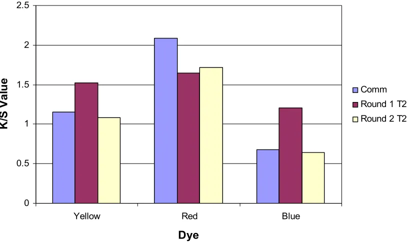
4.2.1 K/S Data ... 49
4.2.1.1 First Round Dyeings ... 50
4.2.1.2 Second Round Dyeings ... 52
4.2.2 Absorption Data ... 55
4.3 WASTEWATER ANALYSIS ... 63
4.4 LEVELNESS ... 64
4.5 FASTNESS ... 65
4.5.1 Colorfastness to Light ... 66
4.5.2 Colorfastness to Water ... 66
4.5.3 Colorfastness to Crocking ... 67
4.6 COST-BENEFIT ANALYSIS ... 68
4.6.1 Dye ... 68
4.6.2 Salt ... 70
5. Conclusions ... 72
6. Recommendations for Future Work ... 74
7. Works Cited ... 75
List of Figures
Figure 1.1 Modification Reaction ... 2
Figure 2.1 Cellulose Repeat Unit ... 5
Figure 2.2 Cellulose Reaction with Dye by Substitution ... 6
Figure 2.3 Type 1 Yellow Dye ... 13
Figure 2.4 Type 2 Yellow Dye ... 14
Figure 2.5 Type 3 Yellow Dye ... 14
Figure 2.6 Type 4 Yellow Dye ... 14
Figure 2.7 Procion® Red MX-8B (CI Red 11) ... 15
Figure 2.8 Procion® Yellow Mx-3R (CI Reactive Orange 86) ... 15
Figure 2.9 Procion® Blue MX-2G (CI Reactive Blue 109) ... 16
Figure 3.1 Quality Control swatches dyed in USA and Poland ... 22
Figure 3.2 NCSU Thies jet dye machine ... 27
Figure 4.1 K/S measurements at varied dye concentrations for yellow dyes ... 41
Figure 4.2 K/S measurements at varied dye concentrations for red dyes ... 42
Figure 4.3 K/S measurements at varied dye concentrations for yellow dyes ... 43
Figure 4.4 Fabric samples from laboratory 0.5% and 2.0% dyeings ... 44
Figure 4.5 % Exhaustion values for lab 0.5% dyeings ... 46
Figure 4.6 % Exhaustion values for lab 2.0% dyeings ... 46
Figure 4.7 K/S values for salt trial dyeings in the lab ... 47
Figure 4.8 Fabric samples from salt trials ... 49
Figure 4.9 K/S values for 0.5% pilot plant first round dyeings ... 50
Figure 4.10 K/S values for 2.0% pilot plant first round dyeings ... 51
Figure 4.11 Fabric samples from first round pilot plant dyeings ... 52
Figure 4.12 K/S values for 0.5% pilot plant dyeings ... 53
Figure 4.13 K/S values for 2.0% pilot plant dyeings ... 54
Figure 4.14 Fabric samples from pilot plant dyeings ... 55
Figure 4.15 % Exhaustion after salt addition for 0.5% pilot plant dyeings ... 58
Figure 4.16 % Exhaustion after salt addition for 2.0% pilot plant dyeings ... 58
Figure 4.17 % Exhaustion after alkali addition for 0.5% pilot plant dyeings ... 59
Figure 4.18 % Exhaustion after alkali addition for 2.0% pilot plant dyeings ... 59
Figure 4.19 Total % Exhaustion after dyeing for 0.5% pilot plant dyeings ... 60
Figure 4.20 Total % Exhaustion after dyeing for 2.0% pilot plant dyeings ... 61
Figure 4.22 Photos of spent dyebath samples for 2.0% dyeings ... 62
Figure 4.23 ADMI color values for wastewater samples from 0.5% dyeings ... 63
Figure 4.24 ADMI color values for wastewater samples from 2.0% dyeings ... 64
Figure 4.25 Cost per pound of production for 0.5% dyeings ... 69
Figure 4.26 Cost per pound of production for 2.0% dyeings ... 70
List of Tables
Table 3.1 Chemical list and suppliers ... 20
Table 3.2 Laboratory dyeing procedure outline ... 24
Table 3.3 Laboratory washing procedure ... 25
Table 3.4 First round pilot plant dyeing procedure outline ... 29
Table 3.5 Adjusted pilot plant dyeing procedure outline ... 32
Table 4.1 K/S values for laboratory dyeings ... 40
Table 4.2 Shade matched percent dyeings (OWG) for both dye types ... 44
Table 4.3 G dye per 25 yd lot needed to obtain commercial K/S values ... 45
Table 4.4 % Exhaustion values for laboratory dyeings ... 46
Table 4.5 K/S values for first round pilot plant dyeings ... 50
Table 4.6 G dye used for first and second round pilot plant dyeings ... 53
Table 4.7 K/S values for all pilot plant dyeings ... 53
Table 4.8 % Exhaustion achieved from addition of salt for pilot plant dyeings ... 56
Table 4.9 % Exhaustion achieved from addition of alkali for pilot plant dyeings ... 57
Table 4.10 % Exhaustion values after dyeing for pilot plant dyeings ... 57
Table 4.11 ADMI color values for wastewater simulation samples f all dyeings ... 63
Table 4.12 Levelness measurements for pilot plant dyeings (σL) ... 65
Table 4.13 Levelness measurements for pilot plant dyeings (σa) ... 65
Table 4.14 Levelness measurements for pilot plant dyeings (σb) ... 65
Table 4.15 Colorfastness to light results for pilot plant dyeings ... 66
Table 4.16 Colorfastness to water results for pilot plant dyeings ... 67
Table 4.17 Colorfastness to crocking results for pilot plant dyeings ... 68
Table 4.18 Cost of commercial and type 2 dyes ... 68
Table 4.19 Cost of materials for production, salt held constant ... 69
1. Introduction
Reactive dyes are among the most common dye type used in the dyeing
of cotton. Although there are many dyes commercially available, the use of
these dyes leaves excess pollutants in the wastewater after dyeing, principally,
salt and color. The treatment of these pollutants is costly and difficult to conduct.
One alternative is to increase the inherit affinity of dyes, thus increasing their
exhaustion and fixation, allowing a dyer to use less salt and dye and reduce the
residual color in his wastewater.
Homobifunctional reactive dyes, synthesized through modification of
commercially available dyes showed improved exhaustion and fixation in lab
experiments (3). The purpose of this work was to extend previous lab studies
into a pilot plant setting to further evaluate the performance of these modified
dyes. These pilot plant studies used, as a starting point, a procedure that was
determined in the lab to be optimal relative to commercially available dyes and
three modified dyes.
1.1 Background
The use of reactive dyes in cellulosic dyeing is often associated with
higher-than-necessary cost and environmental concerns from the discharge of
color due to inefficient fixation. To achieve an acceptable level of exhaustion and
fixation, high levels of salt are typically used with the reactive dyes currently
available on the market. This increases cost due to the cost of the salt and raw
material, as well as causing costly and difficult wastewater treatment to be
necessary. In addition, high concentrations of salt are very corrosive to batch
Researchers at North Carolina State University have been working with
derivatives of commercially available fiber reactive dyes that exhibit higher
affinities, but have the same fastness and color as the parent dyes (3). These
dyes have much greater exhaustion on cotton with greatly reduced amounts of
salt. Commercial dichlorotriazine dyes can be modified to form high-affinity
modified versions by adding steps to the dye manufacturing process. The
modification involves adding additional triazine rings to the dye molecule, thus
increasing its size. When this is done in a way that allows the rings to lay in the
same plane as the parent dye molecule, higher affinity results. The reaction is:
Fig. 1.1 Modification Reaction
Extensive analysis on this new dye form and its application has been
completed in the lab. Four modified dye types were studied for each of three
commercially available dyes. This lab work, completed by R. Berger, an Institute
of Textile Technology (ITT) Fellow at North Carolina State University, identified
reactivity, salt sensitivity, and temperature sensitivity. That work also included
characterization of each dye’s fastness and thermodynamic properties. An
optimized dyeing procedure was established that allows higher exhaustion and
fixation with less salt. These studies identified the optimal time, temperature, and
levels of auxiliaries for the dyeing process.
This research focused on further understanding the practical application of
the best modified dye type identified in the work completed by R. Berger,
specifically:
1. to replicate Berger’s work
2. to evaluate levelness and application properties of the modified dyes
3. to apply the modified dyes in a jet machine at low bath ratio.
This allowed not only for confirmation of lab findings in a pilot-plant setting, but
also gave a better understanding of the optimal dyeing process and realistic use
of the modified dye. This research evaluated the color, levelness, and fastness
of the fabric dyed with the modified dye on pilot-scale machinery. This work also
provided data necessary for cost analysis of the modified dyes, thus allowing an
estimate of economic feasibility.
1.2 Specific Research Objectives
The specific goals of this research were:
1. Optimize the dye procedure for the modified dyes
2. Determine the physical properties and overall performance of the
modified dyes relative to commercially available dyes on a realistic
3. Determine the levels of dye and salt in wastewater for commercial
versus modified dyes.
4. Determine the relative economics of the modified dyes relative to the
commercially available reactive dyes, including the cost savings from
the improved dyeing situation, as well as any changes in the cost of
the dyestuff manufacturing process.
2. Literature Review
2.1 Cellulosic Fibers
Cellulose is a very common raw material in textiles; it is a plentiful naturally
occurring fiber. There are many types of cellulose-based fibers used in textiles,
including cotton, flax, hemp, jute, and regenerated cellulosic fibers such as
Rayon (9).
2.1.1 Structure of Cellulose
The structure of cellulose allows certain benefits of its use in textile
products. The degree of polymerization of the natural cellulosic molecular chain
is of the order of 10,000, and the average cellulosic fiber is about one third
amorphous (8). This amorphous region causes cellulosic fibers to be highly
absorbent fibers; this is a desired attribute in many textile end uses.
Fig. 2.1 Cellulose Repeat Unit
The molecular structure of cellulose, seen in Figure 2.1, contains carbon,
oxygen and hydrogen (14). Two anhydroglucose rings bonded together by an
is made up of three hydroxyl groups (14). The hydroxyl groups allow hydrogen
bonding from chain to chain, which aids in stabilizing the fiber (8).
2.1.2 Cellulose in the Presence of Alkali
Cellulose reacts with dye to form covalent bonds by nucleophilic
substitution or addition. This chemistry is initiated with the treatment of cellulose
with an alkali to form an anionic cellulose nucleophyle. When cellulose is treated
with alkali, an anion is formed. This negative charge is attracted to the positive
site in the dye structure and is capable of reacting with a dye molecule through
either nucleophilic substitution or addition (7). The bond formed is a covalent
bond. This reaction allows for the dyeing of cellulose fiber and fabrics. In the
case of the current dyes, the reaction is a substitution, as shown in Figure 2.2.
Fig. 2.2 Cellulose Reaction with Dye by Substitution
2.2 Reactive Dyes
In 1956 a new class of dyes for cellulosics was introduced commercially;
this new dye class chemically reacted with cellulose. While these new dyes were
more costly and left a large amount of dye unfixed, they were quite popular for
bright shades and versatility of application (7). Research completed by Rattee
and Stephen in 1953 supported the formation of a covalent bond between these
ionic and hydrogen bonds of other cellulose dyes, thus improving fastness
properties. It also provided much improved fastness properties when compared
to traditional ways of attaching dyes to fiber, which were physical absorption or
mechanical retention (19). The reactive dye class was the only class that could
achieve this covalent bond with a substrate upon application (13). Reactive dyes
have also been used to dye wool and other fibers such as polyamide, but these
quantities are small when compared to the quantities used for cotton dyeings
(17). No other single dye class can produce the full range of brilliant colors on
cotton substrates that is available with reactive dyes (12).
2.2.1 History of Reactive Dyes
Textile dyers have been for years faced with the challenge of achieving
lifetime quality of product; this is to say to match the permanence of dyeings with
the useful life of the fabric dyed. Dyeing with available dyes prior to 1950 was
greatly limited by physical absorption or mechanical retention of the dye by the
fiber. Several pre-treatments and after-treatments were developed in an attempt
to improve the fastness of the available cellulosic dyes.
While wool and cotton both have reactive groups present in their
structures, developments in reactive dyes focused mainly on wool until the
1950’s. A wide variety of successful shades were already achievable with wool,
however, these dyeings were not successful with cotton fibers (2). Years of
research went into the development of a successful cotton reactive dye. Nearly
60 years after the initial research was begun, a viable system for achieving a
covalent bond between a reactive dye and cellulose in simple aqueous
commercial reactive dyes in 1956, capable of being applied to cellulose under
cold dyeing conditions (20-40 °C). The patents for these dyes were owned by
ICI, and they were named Procion® dyes. Other commercial reactive dyes were
introduced soon after this initial market penetration, including Cibacron® dyes by
Ciba and Remazol® by Hoechst (2).
2.2.2 Molecular Structure
The structure of triazine reactive dyes is made up of a chromogen, which
provides the color, which is connected to a reactive group and leaving group by a
bridge. The anionic cellulose displaces the leaving group by nucleophilic
substitution. This allows the reactive group to react with the resulting hydrogen
through substitution or addition. This reaction imparts dye color to cellulosic fiber
(7). One problem associated with this interaction is that alkaline hydroxyl groups
in the water (OH--) also are reactive nucleophilic, and they compete with the
hydroxyl group in the cellulose. Thus some of the dye molecules bond with these
hydroxyl groups through hydrolysis. Approximately 10-40% of the dye is lost to
hydrolysis during a reactive dyeing and is not attached to the cellulose molecule
(7).
There are several differentiating structural properties when considering
reactive dye molecules. There are several different chromophores, reactive
groups, and leaving groups that can be used to form reactive dyes. These
groups are used to categorize fiber reactive dyes into specific subclasses. The
dyes used in this research are dichlorotriazine dyes, with dichlorotriazinyl
reactive groups, meaning they have two chlorine atoms which react with the
2.2.3 Application of Reactive Dyes
The choice of dye class is based on desired quality and economics of the
end use product. If fiber reactive dyes are selected, the choice of sub-class is
dictated by production factors, specifically equipment availability, which affects
bath ratio, temperature capabilities, etc. Dye temperature and liquor ratio are
usually determined by the needs of the equipment and the substrate to be dyed
(12).
Optimal batch and continuous procedures for the application of reactive
dyes have been established based on known factors in dyeing, such as rate of
fixation, efficiency of fixation, and reactivity. Batch methods are most commonly
used, and a traditional batch procedure can be broken down into three steps (9).
These three steps are:
1. Exhaustion from an aqueous bath under neutral conditions in the
presence of salt at elevated temperatures.
2. Addition of alkali to promote further uptake and chemical reaction of
dye with fiber at elevated temperatures.
3. Salt, alkali, and unfixed dye are removed through rinsing and
soaping.
Regardless of temperature, a reactive dyed fabric must be washed to remove the
unfixed exhausted dye (12).
2.2.3.1 Electrolytes
Without the presence of electrolyte, exhaustion of dye onto a substrate in
a neutral solution is very low (2). The dye reacts more with water (OH--) in the
dyebath disrupts the molecular structure of the water. This reduces the hydration
of dye in the dyebath and hydrogen bonding sites in the fiber. The result is
exhaustion of dye onto the fiber. Electrolytes used in exhaust dyeing are
common salt (sodium chloride) and Glauber’s salt (sodium sulfate). It has been
shown that at several different concentrations, exhaustion was directly
dependant upon salt concentration (3, 9). It is important to note that increasing
salt concentration has a decreasing effect, thus very high concentrations of salt is
uneconomical (6).
Salt is typically added in the dry state unless large amounts are needed.
In this case, it is advantageous to dissolve the salt before addition to the dyebath.
Producing and handling brine as opposed to dry salt can be less labor intensive
and costly (9). However, using brine can be more risky due to the more rapid
action of brine, which produces the potential for streaky dyeings. The amount of
salt required for a reactive dye process is generally four times the amount
required for a direct dye process (2). Average salt usage in textile manufacturing
with reactive dyes ranges from 50-100% on the weight of the goods (15).
Average salt concentrations range from 70 to 100 g/L on the weight of the bath
for reactive dyeings.
2.2.3.2 Alkali
Under neutral conditions, reactive dyes will fail to form a chemical bond with a
cotton substrate. For this chemical bond to form, alkali is added to the dyebath
to produce more cellulosate ions (2). Once this occurs, the cellulosic substrate is
more capable of reacting with the dye molecules. Cellulose treated with alkali
the dye fixes on the fiber and is resistant to washing and rubbing. Before alkali is
added, the dyeing system is “almost in a state of equilibrium’ (19). At this time,
dye molecules are still diffusing from the dyebath into the fiber and out of the
fiber into the dyebath. When alkali is added, the diffusion of the dye molecules
out of the fiber stops, and more dye molecules diffuse out of the dyebath into the
fiber, thus increasing the overall fixation of dye in the fiber (19).
Commonly used alkalis include soda ash (anhydrous sodium carbonate)
and caustic (sodium hydroxide). Studies have demonstrated that cellulose
exposed to alkaline solutions forms the anionic/nucleophilic form, sometimes
called “soda cellulose” which is much more reactive with certain reagents,
including dyes (11). Soda ash or caustic is typically dissolved at low
temperatures and added to the dyebath in solution form (9). Concentration of
soda ash used with triazine reactive dyes is typically 10 g/L (5).
2.2.3.3 Bath Ratio
The bath ratio, or liquor ratio, is controlled by the dyer and defined as the
ratio of the weight of the liquid (usually water) used to the weight of the goods
being dyed. Lower bath ratios allow for less hydrolysis in reactive dye processes
as well as more efficient dyeings. Generally a decrease in liquor ratio must be
accompanied by an increase in dye concentration in order to maintain a specific
shade. Common bath ratios in the jet application of reactive dyes in industry
today range from 8:1 to 12:1 (15).
2.2.3.4 Temperature
The temperature of a dye procedure is dependant on the type of dye being
due to high levels of reactivity (12). Lower temperatures allow for a more
efficient dye process. Rattee showed, however, that an increase in temperature
did result in an increase in fixation for these dyes. The same result could be
achieved through an increase in salt concentration as well (10). In general,
higher fixation rates can be obtained in lower temperature dyeings through the
utilization of higher salt concentrations. Average dye temperatures for
dichlorotriazine fiber reactive dyes in textile manufacturing today range from
40-60 °C.
2.2.3.5 Typical Procedure
The following procedure is commonly used for a commercial reactive dye
application today (5). This procedure is for a 2.0% exhaust dyeing on 100%
cotton:
1. Fill dye container with water
2. Add cloth
3. Add pre-dissolved dye
4. Add 70 g/L common salt
5. Raise temperature 2 °F per minute to 105 °F
6. Run 15 min
7. Add 10 g/L soda ash
8. Run 45 min
9. Drop bath
10. Rinse hot for 2 min and drop bath
11. Soap at 200 °F for 15 min and drop bath
It is accepted practice to add salt and soda ash in increasing parts over an
average period of 10-15 min (9).
2.2.4 New Reactive Dyes
New homobifunctional reactive dyes were patented by Procter and
Gamble in 2002, and offer improved performance above traditional reactive dyes.
A bifunctional dye is one that has two reactive groups, allowing further reaction
with the substrate (13). A homo-bifunctional dye implies that the two reactive
groups are alike (13). There are currently four new dye types that are still in the
stages of investigation. Figures 2.3-2.6 are the new reactive dye structures for
the yellow versions.
Figure 2.4 Type 2 Yellow Dye
N
N NH N
N N
Cl
SCH2CHNH N
N N
Cl
NH N
N SO3H
HO3S
SO3H
HN O H2N
COOH
NH O
NH2
HO3S
HO3S
SO3H
Figure 2.5 Type 3 Yellow Dye
N
N NH N
N N
Cl
SCH2CH2NH N N N
Cl
NH N
N SO3H
HO3S
SO3H HN
O H2N
NH O
NH2
HO3S HO3S
SO3H
Preliminary research has determined that some of these new dye types provide
higher levels of exhaustion and fixation relative to traditional fiber reactive dyes.
This preliminary testing has also shown that the dyes required lower electrolyte
concentrations and temperatures, and dyed samples possessed good fastness
(3).
Suggested for synthesis and trials of these new dye types are the
commercially available Procion® dyes. These dye structures are shown in
Figures 2.7-2.9(3).
Figure 2.7 Procion® Red MX-8B (CI Reactive Red 11)
Figure 2.9 Procion® Blue MX-2G (CI Reactive Blue 109)
2.2.5 Past Work
Recent research completed by R. Berger, ITT Fellow, at NCSU
determined which of the modifications of the commercially available reactive
dyes offered an increased level of affinity and efficiency of fixation. Specific
objectives of her work included:
1. Evaluate the performance of the four modified dye types
2. Develop an optimal dye application process for the most promising
structure
Experiments were conducted using the three commercially available reactive
dyes and the four modified dye types (3).
2.2.5.1 Optimized Laboratory Dye Process
Previous laboratory dyeings were conducted with the modified dye type
using an Ahiba Texomat laboratory dyeing machine (3). Dyeings were done at
0.25% and 1.0% (owg) with a liquor ratio of 40:1. Deionized water was added to
each Texomat tube in the amount of 200 mL, followed by the appropriate addition
machine at 30°C. The fabric samples were mounted on Ahiba sample holders
and placed in the baths to agitate. The temperature was increased to 30, 60, or
90°C at the maximum rate of rise and held for 5 min. The baths were then
cooled at the maximum rate of cooling to the desired dyeing temperatures and
held for 10 min. Various amounts of salt were added to the tubes in two doses
spaced 1 minute apart. Dye exhaustion was continued for 15 min before alkali
was dosed over a 15 minute time period. Dyeing was then continued for 30 min.
Fabric was then removed and samples of the dye baths were placed in sealed
containers for subsequent analysis (3).
2.2.5.2 Results and Conclusions of Past Work
Berger’s exhaustion experiments yielded affinity and substantivity data for
all dye types. With this preliminary data she found that the type 2 and the type 4
dye structures had higher affinity relative to the commercial dyes and other two
modified structures. Further investigation was then conducted with these two
dye types. Lab dyeings yielded K/S data, fixation ratios, and percent fixation
data. Berger determined that the type 2 dye structure offered better performance
with no negative effect on the fastness performance of the dyed fabric (3).
2.3 Pilot Plant Thies Dye Jet
The Thies fabric “mini-soft” dyeing machine was created for dyeing
samples and small batches. This machine accurately represents dyeings in a
production plant (18). A minimum liquor ratio of 1:5 is recommended by the
manufacturer, and fairly high liquor ratios can successfully be obtained.
Maximum operating temperature is suggested by the manufacturer to be 140 °C
The “mini-soft” was created specifically to allow the capability of
reproducing the wet processes found in a production plant today. The unit is
equipped with electronic temperature control, adjustable liquor quantity,
adjustable winch speed and resulting fabric speed.
2.4 Environmental Concerns
Reactive dyes present two main environmental concerns: color in
wastewater and high salt concentrations. US textile manufacturers using
reactive dyes today face regulations that limit salt concentrations in rivers to 480
ppm. High salt concentrations required for fiber reactive dyes lead to typically
3,000 ppm of salt left in wastewater post-dyeing (15). This salt is diluted when it
enters the receiving stream, but when many discharges put salt-laden waste
streams into a river, eventually the US EPA limit will be exceeded.
One case study conducted by the EPA showed that mill producing about
400,000 pounds per week discharged over 50,000 pounds of salt in a 6-week
period (15). This computes to approximately 433,000 pounds of salt discharged
into the wastewater in one year. Environmental controls impose limits on the
amount of salt in wastewater discharged to a publicly owned treatment works of
as low as 250 ppm (15). It is extremely costly for a facility to lower the amount of
salt in its wastewater to low levels near 250 ppm. Reducing the salt in the
wastewater by reducing salt use would be a more efficient manner of dealing with
environmental concerns.
Another environmental concern is the amount of color remaining in the
wastewater after dyeing. An average ADMI color value for wastewater from a
approximately 15-40% of the dye can hydrolyze, failing to fix on the fabric and
remaining in the dyebath. This dye is discharged with the spent dyebath as color
in the wastewater. This color is not only an aesthetic pollutant, but it can also
inhibit the penetration of light into lakes and rivers, thereby affecting plant growth.
Also, some dyes are toxic to aquatic life. Treatment to remove this color from the
wastewater is costly and not very effective. This color can also interfere with
public waste treatment operations (16). In the early 90’s dyers and dye
manufacturers began focusing on modified dyes that require only about 60% on
the weight of goods salt concentration with approximately 90% exhaustion (4).
Dye modification is the most cost effective way of reducing the amount of color
3. Experimental Plan and Methodology
3.1 General Information
Approximately 600 yd of fabric was used for this research. Dyeings were
conducted with 100% cotton tubular jersey knit fabric weighing approximately 5.6
oz/yd². The fabric was fully prepared by Russell Athletics (bleached and
scoured) before it was donated. When the fabric was received, it was cut into 25
yd pieces and stored until dyeing. The commercially available dyestuffs as well
as the modified dyes were manufactured by the Institute of Dyes and Organic
Products in Poland. Approximately 5 kg each of Reactive Orange 86, Reactive
Blue 106, and Reactive Red 11 were purchased. A portion of the dyes were
converted to the modified type 2 structure by the dye manufacturer before
shipping. All commercial and type 2 dyes used in this research were purchased
from the same dye manufacturer. The chemicals used in this research included
sodium chloride (referred to as salt), sodium carbonate (soda ash), Triton X-200
(scouring agent), and water. The dyeings were conducted in a Thies Jet in the
NCSU COT pilot plant. The city water supply to the pilot plant was determined to
be of sufficient quality for use in this research. Table 3.1 lists the chemicals used
and the suppliers.
Table 3.1 Chemical list and suppliers.
Chemical Supplier
Sodium Chloride - Food Grade Morton
Sodium Carbonate - 100 Grade FMC Wyoming Corporation
3.2 Quality Control Testing
3.2.1 Fabric Testing
The fiber content of the fabric used for this research was tested according
to AATCC Test Method 20 and determined to be 100% cotton knit fabric. The
fabric was 22.5 inches wide tubular, 5.605 oz/sq. yd., and 2.284 yd/lb. The stitch
count was 32 courses and 30 wales per inch. The absorption of the fabric was
tested according to AATCC Test Method 79. The pipette released 18 drops/mL,
and 5 readings were taken at each of 10 different places measured on the fabric.
The average absorption time was determined to be 1.7 seconds.
The pH of the fabric was measured according to AATCC Test Method 81
with a Thermo ORION meter, Model 290A, which was calibrated with a 7.0 and
4.0 buffer solution. A 10 (+/- 0.1) g sample of the fabric was measured was
determined to have a pH of 9.6. The alkalinity of the fabric was tested according
to AATCC Test Method 144. Two samples were tested, and the alkalinity of the
fabric was calculated as 8.34%. The ash content of the fabric was determined
according to AATCC Test Method 78 to be .003%.
The fabric that was donated for this research was tested to ensure that it
had been fully prepared. Reactive dyes are very sensitive to chlorine, so it was
vital that the fabric and the water used for the dyeings be free of this agent. All
3.2.2 Dye Testing
Dyes used in this research were quality tested with the manufacturer
before order fulfillment. These quality control tests were conducted to ensure the
manufactured dyes would meet or exceed shades achieved with dyes
manufactured at NCSU for previous research. Quality control swatches were
received by NCSU from the dye manufacturer.
Figure 3.1 shows the quality control swatches that were dyed at NCSU in
the USA and the Institute of Dyes and Organic Products in Poland. It was
determined that the dyes manufactured in Poland were darker in shade than the
dyes manufactured at NCSU.
3.3 Laboratory Dyeings
Preliminary studies were conducted in the lab in order to better
understand the properties of the commercially manufactured type 2 reactive dye
modification. Laboratory dyeings with both the commercial and modified dyes
were conducted on a Pyrotec Roaches dye machine according to the procedure
listed in Table 3.2. Cotton fabric was cut into 25 g (+/- 0.1) samples, and the
second liquor ratio obtained was 10:1 in order to simulate pilot plant
specifications. Fabric samples was loaded into the chambers with 200 mL of
water and rinsed before the dye solution was added. After rinsing, the bath was
dumped and water was extracted from the samples.
Appropriate amounts of dye were dissolved in 200 mL aquatic solutions
and added to the dye chamber after fabric samples were reloaded. After addition
of pre-dissolved salt and alkali, described below, the total bath volume was 250
mL, giving a 10:1 second bath ratio. Commercial dyeings were conducted at 0%,
0.5% and 2.0% on the weight of the goods. Modified type 2 dyeings were
conducted at 0%, 0.5%, 1.0%, 1.5%, 2.0% and 3.0% on the weight of the goods.
Table 3.2 Laboratory dyeing procedure outline.
Step Description (min) Time Temperature (Celsius)
1 Load dye container with fabric and water 1 -
2 Heat at maximum rate of rise 4 30
3 Run 10 30
4 Drop bath and extract water from fabric 1 30
5 Load fabric and dye bath 1 30
6 Heat at maximum rate of rise 4 60
7 Run 10 60
8 Add 1/3 of salt solution to dyebath 1 60
9 Run 15 60
10 Add remaining salt solution to dyebath 1 60
11 Run 15 60
12 Add 1/5 of alkali solution to dyebath 1 60
13 Run 10 60
14 Add 1/3 of alkali solution to dyebath 1 60
15 Run 10 60
16 Add remaining alkali solution to dyebath 1 60
17 Run 20 60
3.3.1 Salt
Both the commercial and modified dyeings were conducted at 40 g/L salt
concentration. This salt concentration was determined optimal for the type 2 dye
modification in previous research completed by Berger. Appropriate amounts of
a saturated sodium chloride solution were added to the dye chamber in two
separate doses over a period of 15 min according to the scheme described in
Table 3.2.
3.3.2 Alkali
The second concentration of alkali was 10 g/L for each of the dyeings.
Again, this concentration of soda ash was taken from previous work by Berger.
Appropriate amounts of a saturated sodium carbonate solution were added to the
3.3.3 Temperature
The temperature of dyeing for the lab dyeings was 60 °C in order to
simulate pilot plant conditions. This temperature was previously determined to
be optimal for application of the type 2 reactive dye modification.
3.3.4 Washing Procedure
The fabric samples were washed after dyeing by first stirring them in cold
tap water immediately after dyeing. Excess water was removed by blotting
before the samples were placed in a hot wash with 0.25 g/L of Triton X-200.
Samples were then transferred to a clean warm bath for rinsing. Before drying
samples were cold rinsed and excess water was extracted by blotting. Samples
were then dried at 120 °C in a Despatchoven for 10 min. Samples were allowed
to condition at room temperature for 24 h before evaluation and testing.
Table 3.3 Laboratory washing procedure.
Step Description (min) Time
1 Place fabric in cold water and agitate 2
2 Transfer fabric into 60 °C water with Triton X-200 and agitate 3
3 Transfer fabric into clean warm water and agitate 2
4 Rinse in clean cold water 1
5 Remove excess water 0
6 Dry 8
3.3.5 K/S Data Collection
K/S measurements were taken on the dried and conditioned fabric
samples using a Datacolor Spectraflash SF600X instrument equipped with
3.3.6 Absorption Data Collection
Absorption measurements were taken on conditioned samples on a Cary
3E UV-Visible Spectrophotometer. The maximum absorption was recorded for
each of the spent dyebaths from the lab dyeings. Absorption data was read to
established calibration curves to determine concentration of dye in the solution
for spent dyebaths from each dyeing.
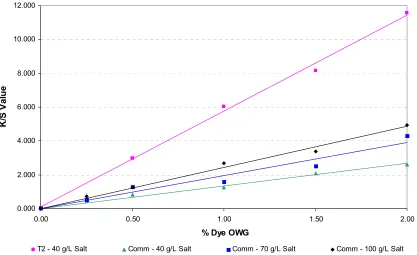
3.3.7 Salt Trial
In order to better understand the relationship of the modified dyes to the
commercial dyes in respect to salt sensitivity, dyeings were conducted with blue
commercial and modified dye at 0.25%, 0.5%, 1.0%, 1.5%, and 2.0% on the
weight of goods. The type 2 blue dyeings were conducted with 40 g/L salt as in
all laboratory and pilot plant dyeings. The commercial blue dyeings were
conducted at 40 g/L, 70 g/L, and 100 g/L salt. K/S values were obtained for each
dyeing.
3.4 Pilot Plant Dyeings
Two steps were completed in the pilot plant at NCSU. An initial round of
dyeings was conducted based on laboratory results and using a dye procedure
similar to that of the lab dyeings. After the dyed fabric was evaluated, a second
round of dyeings was completed using an adjusted dye procedure and optimized
type 2 dye concentrations.
3.4.1 First Round Dyeings
Initial dyeings were conducted with each of the three individual
commercial dyes (red, yellow, blue) at 0.5% and 2.0 %. Appropriate dyeings
order to match the shade obtained in the commercial dyeings. The appropriate
concentrations of dye were determined from laboratory results. K/S values
obtained from lab dyeings were used to create K/S graphs for each color. The
K/S curves for commercial and modified dyes were graphed together. The graph
was used to determine the type 2 dye concentration necessary to obtain the K/S
value obtained with a commercial dyeing of a specific percentage on the weight
of the goods. Dyeing temperature, salt and alkali addition, and hold times were
replicated directly from the laboratory dye procedure, which was taken from
previous laboratory work and adapted to the NCSU COT pilot plant Thies jet
dyeing machine seen in Figure 3.1.
Figure 3.2 NCSU Thies jet dye machine
Table 3.4 outlines the procedure used for the pilot plant dyeings. This
of 10:1 was and 100% cotton knit fabric was dyed in 25 yd lots of 11 lbs each.
Fabric was loaded into the jet for an initial cold rinse before the appropriate
amount of dye was added through the jet add-tank. Dye temperature was 60 °C
and second fixation time was 20 min. The dye procedure ended with two cold
Table 3.4 First round pilot plant dyeing procedure outline.
Step Description Time (min) Temperature (Celsius)
1 Fill dye jet with water 1 30
2 Load fabric 1 30
3 Run 10 30
4 Full drain 3 30
5 Fill with water 1 30
6 Add dye 1 30
7 Heat at maximum rate of rise 8 60
8 Run 10 60
9 Add 1/3 salt solution 1 60
10 Run 15 60
11 Add remaining salt solution 1 60
12 Run 15 60
13 Add 1/5 alkali solution 1 60
14 Run 10 60
15 Add 1/3 alkali solution 1 60
16 Run 10 60
17 Add remaining alkali solution 1 60
18 Run 20 60
19 Full drain 3 60
20 Fill with water 1 30
21 Run 10 30
22 Full drain 3 30
23 Fill with water 1 30
24 Run 5 30
25 Add Triton X-200 1 30
26 Heat at maximum rate of rise 8 80
27 Run 10 80
28 Cool at maximum rate 8 60
29 Run 10 60
30 Full drain 3 60
31 Fill with water 1 30
32 Run 10 30
33 Unload fabric 1 30
Total Process Time 185
3.4.1.1 Salt
A salt concentration of 40 g/L was used for all dyeings. Salt was added in
of 2 kg of salt was dissolved in 7 L of water, and appropriate amounts of solution
were added to the jet through the add tank.
3.4.1.2 Alkali
Ten g per liter of soda ash was added over a period of 20 min in three
separate parts according to the scheme in Table 3.4. A total of 500 g of soda
ash was dissolved in 2 L of water, and appropriate amounts of the solution was
added to the jet through the add tank. It should be noted that due to the addition
of salt and alkali as pre-dissolved solutions, the bath was increased by
approximately 9 L to a ratio of 11.8:1.
3.4.1.3 Temperature
The temperature of dyeing was 60 °C. This temperature was obtained
through maximum rate of rise after the addition of dye to the jet. The maximum
rate of rise on this jet was approximately 4 °C per minute.
3.4.1.4 Wash Steps
Triton X-200 surfactant was added to the jet during the wash step as
outlined in Table 3.4. A total of 0.25 g of surfactant was stirred into 100 mL of
water and added to the jet through the add tank.
3.4.1.5 Fabric Dyeing and Conditioning
Fabric was taken directly from the jet to a centrifugation unit to extract the
excess water. The 25 yd piece was then dried at 70 °C in an ADC dryer, model
number ADS50, for 60 min. After drying, an 8 yd piece was cut from the center
of the dyed piece for evaluation and testing. The sample was hung at room
3.4.2 Second Round Dyeings
A second round of dyeings was conducted with the three individual
modified dyes (red, yellow, blue) using adjusted dye concentrations, adjusted
according to first round dyeing results. The dye procedure was shortened from
185 min to 127 min based on excellent levelness and absorption data from first
round dyeings. The new procedure was less conservative. Decrease in length
of procedure resulted from the decrease in run times between and after salt and
alkali additions. Additional decrease in procedure time resulted from the
decrease in wash times. Concentrations of salt, alkali and surfactant, dye
temperatures, and bath ratio remained the same as in the first round dyeings.
Second dyeings were conducted on the same pilot plant Thies jet dyeing
Table 3.5 Adjusted pilot plant dyeing procedure outline.
Step Description Time (min) Temperature (Celsius)
1 Fill dye jet with water 1 30
2 Load fabric 1 30
3 Run 2 30
4 Full drain 3 30
5 Fill with water 1 30
6 Add dye 1 30
7 Heat at maximum rate of rise 8 60
9 Add 1/3 salt solution 1 60
10 Run 10 60
11 Add remaining salt solution 1 60
12 Run 10 60
13 Add 1/5 alkali solution 1 60
14 Run 10 60
15 Add 1/3 alkali solution 1 60
16 Run 5 60
17 Add remaining alkali solution 1 60
18 Run 15 60
19 Full drain 3 60
20 Fill with water 1 30
21 Run 5 30
22 Full drain 3 30
23 Fill with water 1 30
24 Run 5 30
25 Add Triton X-200 1 30
26 Heat at maximum rate of rise 8 80
27 Run 5 80
28 Cool at maximum rate 8 60
29 Run 5 60
30 Full drain 3 60
31 Fill with water 1 30
32 Run 5 30
33 Unload fabric 1 30
Total Process Time 127
3.4.2.1 Salt
Salt concentration remained the same during the second round of dyeings
scheme in Table 3.5. Salt was dissolved and added to the dye bath in the same
manner as outlined in section 3.4.1.1.
3.4.2.2 Alkali
Second concentration of soda ash was 10 g/L. Soda ash was added over
a period of 15 min in three separate parts according to the scheme in Table 3.5.
Alkali was dissolved and added to the dyebath in the same manner as outlined in
section 3.4.1.2.
3.4.2.3 Temperature
The temperature of dyeing was 60 °C. This temperature was obtained
through maximum rate of rise after the addition of dye to the jet. The maximum
rate of rise on this jet was approximately 4 °C per minute.
3.4.2.4 Wash Steps
Triton X-200 was added to the jet during the wash step as outlined in
Table 3.5. A total of 0.25 of surfactant was stirred into 100 mL of water and
added to the jet through the add tank.
3.4.2.5 Fabric Dyeing and Conditioning
Fabric was taken directly from the jet to a centrifugation unit to extract the
excess water. The 25 yd piece was then dried at 70 °C in an ADC dryer for 60
min. After drying, an 8 yd piece was cut from the center of the dyed piece for
evaluation and testing. The sample was hung at room temperature to condition
for 24 h.
3.5 Color Data Collection
K/S measurements and CIE Lab values were recorded for all fabric
The maximum K/S value and the average Lab value were recorded for each
sample.
3.6 Absorption Data Collection
Absorption measurements were taken on a Cary 3E UV-Visible
Spectrophotometer. The maximum absorption was recorded for samples taken
from the dyebath at three different stages for each dyeing. A sample of 20 mL
was taken after the addition of dye to the dyebath. A second sample of 20 mL
was taken after the addition of salt to the dyebath. A second sample of 20 mL
was taken after second fixation time.
3.7 Wastewater Analysis
ADMI color measurements were taken for each spent dyebath sample.
ADMI Color values were recorded for commercial dyeings and second round
modified dyeings. Wastewater samples were simulated using diluted spent
dyebath samples. The dilution was calculated based on 10 lbs per 1 lb
production water usage reported by the US EPA. Pilot plant dyeings were
conducted with approximately 108 lbs water and 11 lbs fabric. In a production
facility, 11 lbs of fabric would be processed with approximately 917 lbs water.
Thus spent dyebath samples from commercial and second round modified
dyeings were diluted 1:8.455.
Percent transmission readings were taken on a Cary 3E UV-Visible
Spectrophotometer at 438 nm, 540 nm, and 590 nm. ADMI color measurements
were calculated using the appropriate formulas. ADMI color measurements
3.8 Physical Testing Procedures
Physical testing was performed on each fabric sample after drying and
conditioning. The following tests were conducted in line with previous research:
1. Colorfastness to Light – AATCC Test Method 16-1998
2. Colorfastness to Water – AATCC Test Method 107-2002
3. Colorfastness to Crocking – AATCC Test Method 8-2001
3.8.1 Colorfastness to Light
Commercially dyed fabric samples from first round pilot plant dyeings were
tested for colorfastness to light according to AATCC Test Method 16-1998 (1).
Fabric samples from second pilot plant modified dyeings were also tested
according to the same procedure. Samples were placed in an Atlas 3Sun Hi35
High Irradiance Xenon weatherometer and exposed to a Xenon light source for
20 and 40 hour time periods. Color change was analyzed in two ways. The
change in color was calculated as delta E (ΔEcmc) measured on the Datacolor
Spectraflash SF600X. Color change was also evaluated according to AATCC
Gray Scale for Color Change according to AATCC Evaluation Procedure 1 (1).
Samples were rated on a scale from 1 (poor) - 5 (excellent). Color change was
assessed in a Gretag Macbeth Spectralight III instrument using illuminant D65.
3.8.2 Color Fastness to Water
Colorfastness to water was evaluated for fabric samples from first round
commercial pilot plant dyeings and second round modified dyeings. Fabrics
were tested according to AATCC Test Method 107-2002 (1). Samples were
evaluated with multifiber test fabric No. 10 for 18 h at 38 °C. To determine color
evaluated using the AATCC Gray Scale for Evaluating Staining according to
AATCC Evaluation Procedure 2 (1). Each of the six fiber strips from each
multifiber test sample was assigned a rating of 1 (poor) – 5 (excellent).
3.8.3 Color Fastness to Crocking
Fabric samples from first round pilot plant commercial dyeings and second
round pilot plant modified dyeings were tested for colorfastness to crocking
according to AATCC Test Method 8-2001 (1). Testing was conducted using an
AATCC Crockmeter. Color transfer was measured using the 9-step AATCC
Chromatic Transference Scale according to AATCC Evaluation Procedure 8 (1).
Color transference was evaluated in a Gretag Macbeth Spectralight III instrument
using illuminant D65. Samples were rated on a scale from 1 (poor) - 5
(excellent).
3.9 Computational Procedures
3.9.1 Calculation of Shade Values (K/S)
Reflectance (R) measurements at λ max (wavelength of minimum
reflection) were taken for each dye sample using the Datacolor Spectraflash
SF600X. K/S values were calculated for each sample using the following
formula.
3.9.2 Determination of Dye in Solution (cs)
Standard Beer-Lambert Law calibration curves were developed for each
dye used in this research. Dye concentrations were mixed with known
concentrations of 0.04 g/L, 0.06 g/L, 0.08 g/L, 0.12 g/L, and 0.2 g/L. The
absorption of each solution was measured using a Cary 3E UV-Visible
Spectrophotometer, and linear regression was used to develop a calibration
curve. This process was repeated for each dye. Absorption measurements were
taken for each dyebath sample, and the calibration curve for the appropriate dye
was used to determine the dye concentration of the sample solution.
3.9.3 Calculation of Percent Exhaustion (%E)
Percent exhaustion was determined using absorption data obtained from
dyebath samples. Second dye concentration was compared to initial dye
concentration according to formula 3.2.
%E = [(csinitial – cssecond) / csinitial] x 100% 3.2
3.9.4 Determination of Levelness (σ)
CIE Lab values were obtained for each dye sample using a Datacolor
Spectraflash SF600X instrument equipped with SLI-Form® software. A set of 10
Lab measurements were taken in a single place on each fabric sample. The
variation of the 10 measurements for each of the Lab readings was calculated as
σ2instrument for each set of data. The standard deviation was calculated from each
variation value and called σinstrument for each of the Lab sets of data. The standard
the instrument. Lab values were also read 10 times along the length of each
fabric sample at random places on the sample. The variation of these 10
measurements was calculated as σ2overall. This measurement was used to
calculate the standard deviation of the Lab measurements along the length of the
fabric sample (σoverall).
Levelness was calculated by the following equation for each Lab value for
each fabric sample:
σ = (σ2overall - σ2instrument )1/2 3.3
Fabric samples with a standard deviation of less than 0.2 for Lab readings were
considered to be from a level dyeing. Standard deviation values were also
analyzed using ANOVA tests.
3.10 Cost-Benefit Analysis
A cost-benefit analysis was conducted to understand the changes in cost
associated with using type 2 dyes in production. Two main variables were
considered: dye usage and salt usage. Environmental costs are highly variable
from location to location and were thus not included in this cost analysis. Costs
of the commercial and modified dyes were obtained from the dye manufacturer
from which the dyes were purchased for this research. Average costs for salt
and soda ash were obtained from Brenntag, the company from which the
chemicals were purchased for this specific research. The prices were bulk
prices.
The second and optimized dye procedure, including optimized dye
modified dyes. A cost comparison was conducted in order to determine the
losses or savings associated with the application of the modified dyes relative to
commercial dyes. Two dye procedures were also costed based on laboratory
salt trial results. A commercial blue dyeing with 100 g/L salt was costed and
4. Results and Discussion
4.1 Laboratory Results
Laboratory data were analyzed to determine optimal dye concentrations
for modified dyes before moving to the pilot plant. Laboratory dyeings were also
used to validate the proposed dye procedure adopted from previous research.
4.1.1 K/S Data
K/S measurements were used as a determination of shade in evaluating
the dyed fabric samples. Table 4.1 gives the K/S measurements for all
laboratory dyeings. These data were used to develop a regression model for
each dye. The graphs were used to study the strength relationship between the
commercial and modified dyes in order to determine what concentration of
modified dye was needed to match the K/S value obtained in 0.5% and 2.0%
commercial dyeings.
Table 4.1 K/S values for laboratory dyeings.
Dye
Concentration Yellow Red Blue (% owg) Comm Mod Comm Mod Comm Mod
0.00 0.044 0.044 0.031 0.031 0.031 0.031
0.50 1.600 2.537 2.530 3.696 1.232 2.979
1.00 - 5.329 - 8.086 - 6.048
1.50 - 6.376 - 11.489 - 8.168
2.00 7.336 9.005 9.662 13.552 4.001 11.583
*Comm: Commercial Dye *Mod: Modified Type 2 Dye
It was determined that the yellow type 2 dyeings had higher K/S values
relative to the commercially available yellow reactive dye. The regressions for
0.000 2.000 4.000 6.000 8.000 10.000 12.000 14.000
0.00 0.50 1.00 1.50 2.00 2.50
% Dye OWG
K/
S V
a
lu
e
T2 Comm
1.59
Figure 4.1 K/S measurements at varied dye concentrations for yellow dyes.
In all tables and figures, T2 or Mod represents the type 2 dyes and Comm
represents the commercial dyes. The 0.5% and 2.0% type 2 yellow dyed fabric
sample K/S measurements were an average of 40.66% stronger relative to the
0.5% and 2.0% commercial dyeings. It was determined that to obtain a K/S
value of that equal to the K/S value obtained in the 0.5% and 2.0% commercial
dyeings, respectively, dyeings at 0.35% and 1.6% needed to be conducted with
the yellow modified dye.
It can be seen on the graph above the concept that was used to determine
the modified dye concentrations. For example, the 2.0% commercial yellow
dyeing yielded a specific K/S value of approximately 7.3. As can be seen with
value to the modified K/S curve. From this curve, one can see that the
concentration needed for a comparable modified dyeing is only 1.59% on the
weight of goods.
0.000 2.000 4.000 6.000 8.000 10.000 12.000 14.000
0.00 0.50 1.00 1.50 2.00 2.50
% Dye OWG
K
/S Va
lu
e
T2 Comm
Figure 4.2 K/S measurements at varied dye concentrations for red dyes.
The 0.5% and 2.0% type 2 red dyed samples were determined to be on average
43.17% stronger relative to appropriate commercial dyeings. To obtain a K/S
value of that equal to the K/S value obtained in the 0.5% and 2.0% commercial
dyeings, respectively, modified dyeings were calculated at 0.38% and 1.46% on
0.000 2.000 4.000 6.000 8.000 10.000 12.000 14.000
0.00 0.50 1.00 1.50 2.00 2.50
% Dye OWG
K
/S Va
lu
e
T2 Comm
Figure 4.3 K/S measurements at varied dye concentrations for blue dyes.
The type 2 blue dyed fabric samples showed the highest increase in K/S values.
Type 2 blue dyed samples were an average of 165.65% stronger than the 0.5%
and 2.0% blue commercial dyeings. To obtain a K/S value of that equal to the
K/S value obtained in the 0.5% and 2.0% commercial dyeings, it was determined
that dyeings of 0.22% and 0.69% needed to be conducted with the blue modified
Table 4.2 Shade matched percent dyeings (OWG) for both dye types.
Dye Comm Mod
0.5 0.35
YELLOW
2.0 1.6 0.5 0.38
RED
2.0 1.46 0.5 0.22
BLUE
2.0 0.69
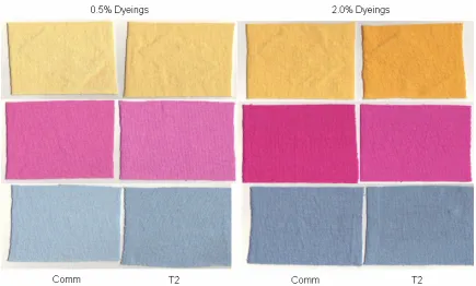
Figure 4.4 depicts the visual difference seen in the 0.5% and 2.0% commercial
and shade matched type 2 laboratory dyed fabric samples. The difference
between the modified and commercial dyes was most evident visually among the
blue samples.
4.1.2 Optimal Dye Concentrations
Based on the K/S regression curves, the optimal concentration of modified
dye for each of the yellow, red, and blue dyes was determined for use in the pilot
plant. Table 4.3 presents the amount of dye calculated that was used for initial
pilot plant dyeings. Commercial dye amounts in g were calculated at 0.5% and
2.0% on the weight of goods. Modified dye amounts in g were calculated to
obtain the same K/S values as each relative commercial dye.
Table 4.3 G dye per 25 yd lot needed to obtain commercial K/S values.
Dye % Dyeing (owg) Comm T2
0.5% 25 17.5
YELLOW
2.0% 100 79.5
0.5% 25 19
RED
2.0% 100 73
0.5% 25 12
BLUE
2.0% 100 34.95
4.1.3 Absorption Data
Absorption measurements were used to determine concentration of dye in
the dyebath before and after dyeing. Absorption measurements were read to
established calibration curves to determine concentration of dye in the solution.
Concentration data from the initial and spent dyebaths were used to calculate
approximate percent exhaustion after dyeing. Table 4.4 gives the % E values
Table 4.4 % Exhaustion values for laboratory dyeings.
Yellow Red Blue
% Dyeing (owg) Comm T2 Comm T2 Comm T2
0.5 57.1 77.8 36.4 88.9 33.3 75.0
2.0 69.2 71.6 52.4 64.3 33.3 72.5
The greatest improvement in percent exhaustion was observed in the 0.5%
dyeings. The modified dyes had on average 75% higher percent exhaustion
values relative to the commercial dyes.
Dyebath samples taken from 0.5% red type 2 dyeings showed the highest
percent exhaustion at 89%. Dyebath samples from the type 2 blue 0.5% dyeings
showed the greatest improvement over the commercial dye at an increase in
percent exhaustion of approximately 125%. For each dye, percent exhaustion
decreased with an increase in dye concentration. Dyebath samples taken from
type 2 blue 2.0% dyeings showed improvements of 118% over commercial
percent exhaustion. All modified dyeings showed improved levels of exhaustion
0 10 20 30 40 50 60 70 80 90 100
Yellow Red Blue
Dye % E Va lu e Comm T2
Figure 4.5 % Exhaustion values for lab 0.5% dyeings.
0 10 20 30 40 50 60 70 80 90 100
Yellow Red Blue
Dye % E Va lu e Comm T2
Figure 4.6 % Exhaustion values for lab 2.0% dyeings.
4.1.4 Salt Trial
K/S values were evaluated for the dyeings conducted at varied levels of