ABSTRACT
GAO, RUI. Control and Design of a PMSG Wind Energy Conversion System and Its Integration with Solid-State Transformer Enabled AC/DC Grid Systems. (Under the direction of Dr. Iqbal Husain.)
The Permanent Magnet Synchronous Generator (PMSG) has been widely adopted for wind renewable generation system, with the single wind turbine power rating ranging from several kilowatt to even ten megawatt. It has the advantages of high efficiency, high power density, and lower maintenance cost for wind energy conversion applications. The back-to-back converter enabled PMSG wind energy conversion system (WECS) outperforms its doubly-fed induction generator (DFIG) counterpart during grid fault situation. However, how to achieve the coor-dinated wind turbine control which consists of the wind generator and the turbine blade pitch angle control, is challenging. The higher penetration of wind energy poses increasing demand for grid support and power management functions of wind energy conversion system (WECS). Aiming at the maximizing the wind energy capture, necessary power curtail, and grid support functions of PMSG WECS, this dissertation addresses the wind turbine system controls, design and applications.
©Copyright 2017 by Rui Gao
Control and Design of a PMSG Wind Energy Conversion System and Its Integration with Solid-State Transformer Enabled AC/DC Grid Systems
by Rui Gao
A dissertation submitted to the Graduate Faculty of North Carolina State University
in partial fulfillment of the requirements for the Degree of
Doctor of Philosophy
Electrical Engineering
Raleigh, North Carolina
2017
APPROVED BY:
Dr. Alex Q. Huang Dr. Srdjan Lukic
Dr. Sharon Lubkin Dr. Iqbal Husain
DEDICATION
BIOGRAPHY
Rui Gao was born in Heilongjiang, China. he received the B.Sc. and M.Sc. degrees in electrical engineering from Harbin Institute of Technology, Harbin, China, in 2009 and 2011, respectively. He started to pursue his Ph.D. degree in North Carolina State University in 2011.
Since 2011, he has been working on the control and design of the wind energy conversion system and its integration with Solid-State Transformer enabled ac/dc grid system at Future Renewable Electric Energy Delivery and Management (FREEDM) Systems center. Starting 2015, he was also involved with the design and development of the high power density and high efficient Silicon Carbide (SiC) traction inverter system sponsored by PowerAmerica Institute. From May to August 2014, he was a research intern with ABB Corporate Research Center, U.S., conducting research on brushless dc motor drive.
ACKNOWLEDGEMENTS
I would like to express my deepest gratitude to my advisor Dr. Iqbal Husain, for his support and guidance in my studies. His technical and editorial advice is indispensable for the completion of this dissertation. I benefited a lot from him not only in terms of the insightful vision for technology, but also his great personalities and leadership, which will keep influencing me in my future career.
My thanks go to all my committee members, Dr. Alex Huang, Dr. Lukic, Dr. Sharon Lubkin, and Dr. Wensong Yu, who have given me lots of valuable suggestions to improve my Ph.D. dissertation. Specially, I would like to thank Dr. Wensong Yu for spending time discussing with me. His passion for research and enthusiasms for techniques really inspire me to go further in the world of power electronics. Meanwhile, the help from other faculties and staffs in the FREEDM systems center are really appreciated.
My thanks also go to my friends and colleagues in FREEDM systems center. It is my great honor to have the opportunities working with those talented minds. I learned a lot from the teammates of electric machine research group and SiC traction inverter design group. Special thanks go to Dr. Xu She, whose insightful suggestion really encourages me during the difficult times, and Dr. Rafael Montoya, whose profound control knowledge always help me clear the hurdles in my research work.
My heartfelt gratitude goes to my parents for their love and support. Family always gives me strength to move forward. Thanks my brother and sister-in-law for supporting me and creating such a warm and happy environment.
Lastly, I would like to thank my beloved wife Suxuan Guo, who worked with me as a colleague. Without her support, this work might not finish. Many times, you are the silver linings in my life. I really appreciate having you by my side.
TABLE OF CONTENTS
LIST OF TABLES . . . .viii
LIST OF FIGURES . . . ix
Chapter 1 Introduction . . . 1
1.1 Overview of Wind Energy Conversion System . . . 1
1.2 Components of Wind Energy Conversion Systems . . . 3
1.3 Types of Wind Energy Conversion Systems . . . 5
1.4 Problem Statement and Research Motivation . . . 8
1.5 Dissertation Outline . . . 10
Chapter 2 Design and Implementation of a 10 HP PMSG WECS . . . 12
2.1 Introduction . . . 12
2.2 Wind Turbine Modeling . . . 13
2.2.1 Wind Turbine Aerodynamic Characteristic . . . 13
2.2.2 Drivetrain Modeling . . . 14
2.3 Wind Generator Control with a Back-to-Back converter . . . 16
2.3.1 Control Methodology . . . 16
2.3.2 Simulation Study . . . 18
2.4 Pitch Controller . . . 25
2.5 Design of a Laboratory Wind Turbine Emulator . . . 26
2.5.1 Development Algorithm . . . 26
2.5.2 Test Results . . . 28
2.6 Implementation and Test of the PMSG Rectifier System . . . 31
2.7 Conclusion . . . 35
Chapter 3 PI Passivity-based Control for PMSG Wind Energy Conversion System . . . 41
3.1 Introduction . . . 41
3.2 System Modeling . . . 43
3.2.1 Wind Turbine . . . 44
3.2.2 Permanent Magnet Synchronous Generator . . . 46
3.2.3 The Overall System . . . 47
3.2.4 Control Objectives as Desired Equilibrium Points . . . 49
3.3 Control Design: The PI-PBC Approach . . . 51
3.3.1 Control Assumptions and Objectives . . . 51
3.3.2 Control Design . . . 51
3.4 Simulation Results . . . 54
3.5 Comparison Study . . . 55
3.5.1 The PI Controller Design . . . 58
3.5.2 Case Study . . . 60
3.7 Improved PI-PBC Method . . . 68
3.8 Experimental Verification of the Improved PI-PBC Method . . . 70
3.9 Conclusion . . . 71
Chapter 4 Standard Passivity-based Control for PMSG Wind Energy Con-version System . . . 77
4.1 Introduction . . . 77
4.2 System Modeling . . . 78
4.3 The Controller Design . . . 79
4.3.1 Control objectives & assignable equilibrium points . . . 79
4.3.2 Copy of the system . . . 82
4.3.3 Zero Dynamics . . . 82
4.3.4 The Controller . . . 84
4.3.5 Final control expression & implementation . . . 88
4.4 Simulation results . . . 89
4.5 Conclusion . . . 91
Chapter 5 Solid-State Transformer Interfaced PMSG Wind Energy Conver-sion System. . . 94
5.1 Introduction . . . 94
5.2 System Modeling . . . 98
5.2.1 PMSG Modeling . . . 98
5.2.2 Solid-State Transformer Modeling . . . 99
5.3 System Control . . . 100
5.4 Simulation Study . . . 101
5.5 Experimental Verification . . . 104
5.5.1 Demonstration of System Integration . . . 104
5.5.2 Modular SST for High Voltage and High Power Application . . . 107
5.6 Conclusion . . . 110
Chapter 6 Distributed Power Management Algorithm for SST Enabled PMSG Wind Turbine DC Network . . . .113
6.1 Introduction . . . 113
6.2 System Control . . . 114
6.2.1 Operation Assumptions . . . 114
6.2.2 System Control Principle . . . 115
6.2.3 Case Studies . . . 120
6.3 Discussions . . . 125
6.3.1 System Adaptability with Energy Storage . . . 125
6.3.2 System Comparison with Conventional WECS . . . 127
6.4 Conclusion . . . 128
Chapter 7 Conclusions and Future Work . . . .130
7.2 Future Works . . . 132
LIST OF TABLES
Table 2.1 System Parameters . . . 25
Table 3.1 Wind system parameters . . . 58
Table 5.1 System Parameters . . . 106
Table 5.2 Parameters of Single Converter Cell based SST . . . 106
Table 5.3 Circuit Parameters of Modular SST . . . 111
LIST OF FIGURES
Figure 1.1 Typical wind turbine structure. (a) conventional windmill [3] . (b) Vertical
axis wind turbine [2]. (c) Horizontal axis wind turbine [40]. . . 2
Figure 1.2 Size Evolution of commercial wind turbines [62]. . . 2
Figure 1.3 Wind turbine system structure [1]. . . 4
Figure 1.4 Basic configuration of a grid-connected wind turbine generation system [62]. 4 Figure 1.5 Type I: fixed speed SCIG WECS [62]. . . 5
Figure 1.6 Type II: WRIG WECS [62]. . . 5
Figure 1.7 Type III: DFIG WECS [62]. . . 6
Figure 1.8 Type IV: Variable speed WECS [62]. . . 6
Figure 1.9 Dissertation outline. . . 11
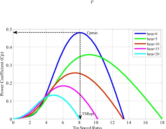
Figure 2.1 Cp-λcurves with various pitch angle. . . 14
Figure 2.2 Turbine power-rotational velocity curves. . . 15
Figure 2.3 Two-mass drivetrain model block diagram. . . 16
Figure 2.4 Back-to-back converter topology. . . 17
Figure 2.5 Control diagram of PWM rectifier. . . 18
Figure 2.6 Control diagram of PWM inverter. . . 19
Figure 2.7 System simulation setup. . . 20
Figure 2.8 Ramping wind speed. . . 20
Figure 2.9 Generator rotational velocity. . . 21
Figure 2.10 Wind turbine mechanical power. . . 21
Figure 2.11 Generator electromagnetic torque. . . 21
Figure 2.12 Generator three-phase currents. . . 22
Figure 2.13 Generator phase-A current. . . 22
Figure 2.14 Generator line-line voltage Vab. . . 22
Figure 2.15 Generator-side rectifierd−axis current. . . 23
Figure 2.16 Generator-side rectifierq−axis current. . . 23
Figure 2.17 Grid-side inverter q−axis current. . . 23
Figure 2.18 Grid-side inverter d−axis current. . . 24
Figure 2.19 Grid voltages. . . 24
Figure 2.20 Grid currents. . . 24
Figure 2.21 Control diagram of pitch controller. . . 26
Figure 2.22 WTE components. . . 27
Figure 2.23 Look-up table explanation. . . 29
Figure 2.24 WTE design flowchart. . . 30
Figure 2.25 Implementation diagram of WTE. . . 32
Figure 2.26 WTE prototyping test setup. . . 32
Figure 2.27 Wind turbine emulator operation waveforms: dc bus voltage, IM Phase-A current, circulating dc current and speed feedback (from up to bottom). . . . 32
Figure 2.29 Wind turbine emulator operation waveforms: dc bus voltage, IM three-phase
currents (from up to bottom). . . 33
Figure 2.30 Wind turbine emulator operation waveforms: dc bus voltage, IM three-phase currents (zoom in, from up to bottom). . . 34
Figure 2.31 Wind turbine emulator operation waveforms: load dc voltage, PMSG phase-A current, load dc current and and speed feedback (zoom in, from up to bottom). . . 34
Figure 2.32 Layout of the WECS controller board. . . 36
Figure 2.33 WECS user interface of FREEDM system SCADA. . . 36
Figure 2.34 Control system hardware components: (a) Interface conditioning board, (b) Control board, (c) ARM board. . . 37
Figure 2.35 Control system hardware components. . . 37
Figure 2.36 Encoder signal (AB). . . 38
Figure 2.37 Encoder index signal with position synchronization. . . 38
Figure 2.38 Position DA (mechanical and electrical) synchronization with phase-A back EMF. . . 38
Figure 2.39 Space vector PWM gating signals (three bottom switch). . . 39
Figure 2.40 Space vector PWM DA output. . . 39
Figure 2.41 System operation waveforms at 200 rpm. Vdc= 380V, Pdc=280 W . . . 40
Figure 2.42 Wind turbine emulator operation waveforms: position DA output, speed DA output, power DA output and PMSG phase-A current (from up to bottom). 40 Figure 3.1 System under consideration . . . 45
Figure 3.2 FunctionCp(λ) . . . 45
Figure 3.3 Block diagram of the control implementation . . . 56
Figure 3.4 Design stages flowchart. . . 56
Figure 3.5 Wind speed profile. . . 57
Figure 3.6 Simulation results. . . 57
Figure 3.7 Standard PI control diagram. . . 59
Figure 3.8 Control performance comparison with constant wind speed. . . 61
Figure 3.9 Control performance comparison with stepping wind speed. (a) Wind speed. (b)daxis current of the PMSG. (c)qaxis current of the PMSG. (d) Generator speed. (e) dc link capacitor voltage. . . 63
Figure 3.10 PI-PBC performance comparison with ramping wind speed (from top to bot-tom). (a) Wind speed. (b) d−axis current of the PMSG. (c) q−axis current of the PMSG. (d) Generator speed. (e) dc link capacitor voltage. . . 64
Figure 3.11 PI Control performance comparison with ramping wind speed (from top to bottom).(a) d−axis current of the PMSG. (b)q−axis current of the PMSG. (c) Generator speed. (d) dc link capacitor voltage. . . 65
Figure 3.12 Improved PI-PBC control diagram. . . 68
Figure 3.14 Waveforms at no load startup. . . 71
Figure 3.15 Steady state operation waveforms. . . 72
Figure 3.16 Load torque step waveforms 1. . . 72
Figure 3.17 Load torque step waveforms 2. . . 73
Figure 3.18 Load torque step waveforms 3. . . 73
Figure 3.19 Load torque step waveforms 4. . . 74
Figure 3.20 System performance waveforms under load torque increase. . . 74
Figure 3.21 System performance waveforms under load torque decrease. . . 75
Figure 3.22 System operation waveforms under speed ramping 1. . . 75
Figure 3.23 System operation waveforms under speed ramping 2. . . 76
Figure 4.1 Plotx4 versus ˙x4 of (4.12) for the different scenarios. Notice that, excluding the case when D=− VS2 4R2 SRe , ¯vc? is always a stable eq. point. . . 83
Figure 4.2 Block diagram of the control implementation. . . 88
Figure 4.3 Simulation results. . . 90
Figure 4.4 Control robustness under parameter variations (time scale: 3 sec/div). . . 92
Figure 4.5 Simulation Results (time scale : 16.7 sec/div). . . 93
Figure 5.1 Conventional integration strategy. . . 96
Figure 5.2 SST based integration strategy. . . 97
Figure 5.3 SST interfaced multiphase-generator structure. . . 97
Figure 5.4 SST interfaced with multiple-generator structure. . . 97
Figure 5.5 System layout diagram . . . 98
Figure 5.6 System control block diagram . . . 101
Figure 5.7 System simulation results under wind speed variation. (a) Wind speed. (b) Generator speed. (c) Pitch angle. (d) High voltage dc bus voltage. (e) Low voltage dc bus voltage. (f) Wind turbine output power. . . 103
Figure 5.8 System simulation results under load step change. (a) Distribution line side input current. (b) Distribution line side input voltage and current. (c) High voltage dc bus voltage. (d) Low voltage dc bus voltage. (e) Generator 3-phase currents. (f) Wind turbine system output power. . . 105
Figure 5.9 Prototype test setup . . . 107
Figure 5.10 VSR operation waveforms with wind speed variation: POI voltage, current, high-voltage and low-high-voltage dc bus. . . 108
Figure 5.11 System operation waveforms with wind speed variation: rectifier dc current, and generator phase A current. . . 108
Figure 5.12 System operation waveforms with constant load: generator phase A current, position signal DA output, and generator line voltageVab. . . 109
Figure 5.13 VSR space vector three-phase PWM reference DA output. . . 109
Figure 5.14 Load step response: generator phase A current and rectifier dc current. . . 110
Figure 5.15 Prototype of modular SST. . . 111
Figure 5.17 System operation waveforms under capacitive-mode: POI voltage, current, PWM
voltage, andVhdc3 . . . 112
Figure 6.1 System layout diagram. . . 115
Figure 6.2 System control block diagram. . . 117
Figure 6.3 System mode transition block diagram. . . 117
Figure 6.4 DBS algorithm flowchart. . . 119
Figure 6.5 Case I system operation. (a) Wind Speed profile. (b) Generator speed. (c) Pitch angle. (d) Turbine output power. (e) DC network bus voltage. (f) High-voltage dc bus. (g) Phse-A High-voltage and current of POI. (h), (i) Three-phase voltages and currents of POI. . . 123
Figure 6.6 Case II system operation. (a) Wind Speed profile. (b) Generator speed. (c) Pitch angle. (d) Turbine output power. (e),(f) dc bus voltage. . . 124
Figure 6.7 Case III system operation. (a) Generator speed. (b) Pitch angle. (c) Turbine output power. (d), (e), (f) dc bus voltage and the zoom-in. . . 125 Figure 6.8 Case IV Reactive power compensation operation. (a) Capacitive mode. (b)
Chapter 1
Introduction
1.1
Overview of Wind Energy Conversion System
Figure 1.1: Typical wind turbine structure. (a) conventional windmill [3] . (b) Vertical axis wind turbine [2]. (c) Horizontal axis wind turbine [40].
1.2
Components of Wind Energy Conversion Systems
The basic configuration of a grid-connected wind turbine generation system is shown in Fig. 1.4. The mechanical components include tower, nacelle, rotor blades, rotor hub, gearbox, pitch drives, yaw drives, wind speed sensors, drive-train and mechanical brakes [62]. The tower and nacelle mainly provide the structure support function. The higher the tower, the more energy the wind turbine can then capture with rotor blades and transformed into kinetic energy for the wind generators. The drivetrain may involve gear-box stage depending on the wind turbine rotor shaft angular velocity and the generator operational velocity. The anemometers are generally used for control and protection requirement. Possible pitch drives are equipped to regulate the blade pitch angles which curtail surplus wind power for security consideration and power demand. Yaw drives are used to regulate the rotor hub towards a upwind direction. The electrical components include an electric generator, a power electronic converter, a grid-side harmonic filter, a step-up transformer and the three-phase grid or transmission point of interconnection (POI).
Figure 1.3: Wind turbine system structure [1].
1.3
Types of Wind Energy Conversion Systems
As seen from Fig. 1.5 to Fig. 1.8, there are four main types of commercial WECS configuration differentiating from the adopted wind generators and are introduced in the following [15]:
Figure 1.5: Type I: fixed speed SCIG WECS [62].
Figure 1.6: Type II: WRIG WECS [62].
Figure 1.7: Type III: DFIG WECS [62].
1%). This technology is simple; however, the SCIG always draws reactive power during normal operation, which is not preferred from power grid. Thus, this configuration has to use a capacitor bank at the generator terminals to compensate the reactive power requirement.
2) Configuration of Fig. 1.6 is in principle the same as the one in type I; however, a wound rotor induction generator (WRIG) with external rotor resistance is utilized in this configuration. This type allows variable-speed operation in a limited range of up to 10% above the grid angular frequency. A capacitor bank is also used in this type for power factor correction. The advantage of this type is its larger slip range compared to type I. The variable speed operation of the wind generator increases the energy capture capabilities. However, the same reactive power compensation structure is needed, which brings in extra cost. Moreover, compared to type I operation, the losses have to increase due to the larger rotor resistance.
3) Fig. 1.7 shows type III configuration where the doubly-fed induction generator (DFIG) can provide a variable-speed operation by means of a partial-scale power-electronic back-to-back converter in the rotor circuit. Depending on the converter size, this configuration allows a wider range of the variable-speed WECS operation of approximately 30% around the grid angular frequency. Moreover, this structure is able to accomplish the reactive power compensation independently. And the small rating of the power electronics converters (30% of the rating) also make this solution attractive. However, this grid fault ride-through capability is limited due to this direct grid interface structure with rotor magnetizing circuit.
1.4
Problem Statement and Research Motivation
The PMSG wind turbine generation system has been widely adopted for real industrial ap-plications. A significant amount of research has done during the past decade. However, the wind turbine system level controls are rarely reported. Most of control work and novel power electronics configurations focus at the wind generator speed control. However, few research publications provide guidelines or design methods for the wind turbine systems. In this work, the overall control variables of the wind turbine system are identified first. And the coordinated wind turbine controls consisting of wind generator and blade pitch actuators are illustrated. Meanwhile, the stochastic and intermittent nature of wind resources makes it difficult or even impossible to conduct research work in laboratory environment. Thus, a 10 Hp prototype WTE is designed and developed for research and education purpose, which is comprised of a 10 Hp induction motor, an ABB ACS800 variable frequency drive (VFD), and a Microchip controller dsPIC24FJ128GA010 for turbine characteristic emulation. The studied wind turbine character is analyzed which involves both static and dynamic response. A low-cost, practical lookup table based method is proposed and implemented for the turbine emulator, and experimental results are provided for justification.
high-voltage and high-power three converter cell based SST are tested in the WECS. The simulated and experimentally verified SST WECS in this research work can be adapted for high-voltage megawatt level wind turbine system. The combination of wide bandgap power devices and the modular structure will further enhance the power and voltage capabilities of the Solid State transformer.
The controller design for wind energy conversion systems (WECS) is complicated consider-ing the nonlinear properties of electric machines (possible flux saturation, machine parameter variations etc.) and power converters. Significant amount of research work has been conducted to address the wind generator controls upon the maximum power tracking, fault tolerant functions, active power flow and reactive power regulation aspects. There are also research publication addressing the dc/ac Microgrid system involving wind turbine generation unit. However, rel-atively less research work tackles with the stability and robustness evaluation of the designed control system. Considering of the flexibility and control freedom that power electronics system brought to wind turbine generation system, it is reasonable to challenge the WECS robustness. How to achieve a controller design with guaranteed stability is critical for real application. Tar-geting this research gap, this dissertation adopts a passivity-based control (PI-PBC) methods for WECS. How to make the advantages of system component interconnection and energy re-shaping concept of this PI-PBC has been detailed addressed. And the controller robustness is proved following Lyapunovs Direct Method.
such control strategy.
1.5
Dissertation Outline
This dissertation focuses on the control and design of the PMSG wind turbine generation system, and its applications in the SST enabled dc/ac grid systems. The organization of the dissertation is shown in Fig. 1.9, the dissertation is divided into seven chapters:
DBS based distributed power management algorithm is elaborated targeting this system. The system grid-connected and islanding mode operation are discussed, demonstrating the potential feasibility of releasing the ESD requirement. Chapter 7 concludes the major contributions of the dissertation and proposes the future work.
Chapter 2
Design and Implementation of a 10
HP PMSG WECS
2.1
Introduction
2.2
Wind Turbine Modeling
2.2.1 Wind Turbine Aerodynamic Characteristic
The mechanical power extracted from the wind and turbine rotor torque are given in (2.1) and (2.2) [26], respectively.
Pw = 1
2ρACp(λ, β)v
3
w (2.1)
Tw =
π
2rρv
2
w
Cp(λ, β)
λ (2.2)
wherevw is the wind speed,ρis the air density,A is the area swept by the blades andCp is the turbine’s power coefficient, which is function of the tip-speed ratio (TSR) λ and the turbine blade pitch angle β. The definitions of TSR and Cp are given as (2.3) and (2.4) [26]. r, ωm represent the turbine rotor radius and mechanical velocity, respectively.
λ= rωm
vw
(2.3)
Cp(λ, β) =c1
c2 λi
−c3β−c4β2−c5
exp
−c6
λi
(2.4)
with fitted values c1= 0.5, c2 = 116, c3= 0.4, c4 = 0, c5 = 5,c6= 21 and
λi =
1
λ−0.035
−1
.
the real time wind speed variation is known. In this paper, this optimal λ is assumed known beforehand. Therefore, when the wind speed input varies, the local wind turbine controllers can calculate and generate the optimal rotor velocity reference for MPPT operation. Equation (2.5) givesωm?andλ?which are the optimal rotor speed reference and the optimal TSR, respectively. Besides, it is seen from Fig. 2.1 thatCp decreases asβ increases, which can curtail the surplus wind power when the wind generation is higher than the present load demand. This essentially forms the basis for turbine blade pitch angle control, which is used for wind turbine protections during extreme weather conditions.
ωm? =
vwλ?
r (2.5)
Figure 2.1: Cp-λcurves with various pitch angle.
2.2.2 Drivetrain Modeling
Figure 2.2: Turbine power-rotational velocity curves.
of gearbox and the low-speed shaft, while the second one consists of the generator mass, high-speed shaft and the other part of gearbox. The dynamic equations are obtained from Newton’s equations of motion for each mass as seen in (2.6) [56, 46],
2Htω˙t=Tm−Tsh 1
ωeB ˙
θtw=ωt−ωr
2Hgω˙r=Tsh−Te
(2.6)
whereHtis the the inertia constant of the turbine,Hg is the inertia constant of the PMSG,
ωr is the angular speed of the wind turbine in p.u.,ωeB is the electrical base speed, θtw is the shaft twist angle, and Tm, Te are wind turbine and generator torque, respectively. The shaft torqueTsh is represented by (2.7),
Tsh=Kshθtw+Dtθ˙tw (2.7)
Figure 2.3: Two-mass drivetrain model block diagram.
2.3
Wind Generator Control with a Back-to-Back converter
2.3.1 Control Methodology
The back-to-back converter structure shown in Fig. 2.4 is generally favored by modern wind turbines because of the decoupling of the generator-side dynamics and the support functionality for the grid-side requirement. As explained in the Chapter 1, the variable speed control can enhance the wind energy utilization efficiency. The downside of this structure comes from the full-scale feature for PMSG based system, which unavoidably increases the overall cost.
The generator-side rectifier control block diagram is shown in Fig. 2.5, where the cascaded control loop structure is observed [16]. The generator rotational velocity command is generated based on appropriated MPPT method to increase the wind energy capture efficiency, and the
currentsisa, isb and position angleθneed to be measured. All the controls are carried out with standard PI compensators.
Figure 2.4: Back-to-back converter topology.
Figure 2.5: Control diagram of PWM rectifier.
The grid-side inverter control block diagram is shown in Fig. 2.6, where similar cascaded control loop can be made. Two main objectives need to be accomplished for the grid-side inverter control, they are dc-link voltage maintenance and the injected reactive power regulation. The
q−axis current reference is adjusted following required reactive power command. Normally, unit power factor operation is generally preferred from inverter perspective. However, during grid voltage dip or fault situations, reactive power compensation function is mandatory for grid-connected renewable generation systems. The output of dq−axis current regulators, together with the rotational compensation items form thedq−axis voltage components. The modulation and reference frame transformation methos follow the same rules as above rectifier control implementation. For feedback component, three-phase grid voltage needs to be measured for the phase synchronization; the line currents and the dc-link voltage are measured for closed-loop control requirement.
It is noted that both machine-side rectifier and grid-side inverter control are implemented in the rotational reference frame, namely dq vector control. However, the q−axis is the active power axis for rectifier and thed−axis is the active power axis for inverter. The former is usually named as rotor flux oriented control, while the latter is named as voltage orientated control. This vector control method has the advantages of fast response, wide speed/voltage operation range, robustness, and decoupled dynamics for both sides.
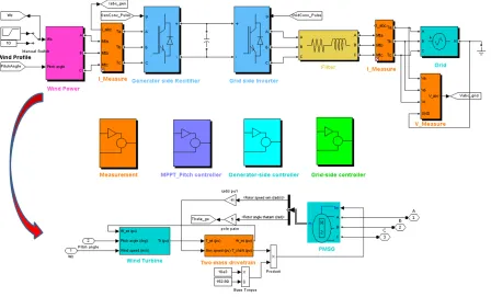
Table 2.1: System Parameters
Wind Turbine PMSG
Air density 1.225 kg/m3 No. of poles 4
Blades radius 3.5 m Rated power 10 kW
vw range 3−15 m/s Stator resistance 0.425 Ω
Gear ratio 1 : 7.3 Stator inductance 8.5 mH
Rated power 18 kW Rated speed 153 rad/s
Shaft stiffness 1 p.u. Flux linkage 0.433 Wb
Shaft damping coefficient 0.3 p.u. Generator inertia constant 0.014 s Turbine inertia constant 0.2 s
Converters & Electrical Parameters
DC link voltage 700 V DC link capacitance 3300uF
Grid voltage (Ph-Ph) 400 V Filter inductance 10 mH Filter resistance 0.1 Ω Switching frequency 10 kHz
2.3.2 Simulation Study
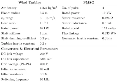
To further verify this benchmark control method, the back-to-back based PMSG grid-connected wind generation system is modeled with Matlab/Simulink, and the system simulation study is conducted considering an arbitrary variable wind speed condition and a unity power factor at grid side. The considered system parameters are given in Table 2.1. The simulation setup is shown as in Fig. 2.7, where it is mainly comprised of wind power block, back-to-back converter block, line filter, and power grid. The wind power block contains wind turbine model, two-mass drivetrain model, and the PMSG model as subsystem. The corresponding control blocks are sequentially shown at the bottom.
in a prompt way, and the static error is zero. A practical regulation can be achieved. Fig. 2.10 presents the extracted wind power, which follows the wind speed profile. Fig. 2.11 shows the PMSG electromagnetic torque output, where the negative value represents the generation condition. Figs. 2.12 and Fig. 2.13 show the PMSG current profile in a full time range and a zoom-in style; Fig. 2.14 shows the machine line-line voltage switching waveforms under 700 V dc link. Figs. 2.15 and 2.16 present the generator-side rectifier dq axis current regulation performance. Comparatively, Figs. 2.18 and 2.17 show the grid-side inverter dq axis current regulation performance. From the power flow perspective, it can be clearly observed that the rectifier q−axis current and inverterd−axis current share the same shape following the wind power variation. Grid-side three-phase voltage and current waveforms are shown in Fig. 2.19 and Fig. 2.20, respectively. And a clear unity power factor operation is observed from the phase relation of the grid voltage and current.
Figure 2.8: Ramping wind speed.
Figure 2.9: Generator rotational velocity.
2.4
Pitch Controller
Figure 2.10: Wind turbine mechanical power.
Figure 2.11: Generator electromagnetic torque.
Figure 2.13: Generator phase-A current.
Figure 2.14: Generator line-line voltageVab.
Figure 2.16: Generator-side rectifier q−axis current.
Figure 2.17: Grid-side inverterq−axis current.
Figure 2.19: Grid voltages.
control functions for over-speed and over-power protection. At circumstances where the load demanding is less than the generation, the power curtailing can be carried through the pitch controls too. The simulation proof of such functions is demonstrated in the chapter 5 together within the power management algorithm frame, and for format wise, the controller is presented here for integrity and logic coherence.
Figure 2.21: Control diagram of pitch controller.
2.5
Design of a Laboratory Wind Turbine Emulator
Considering the stochastic nature of the wind resources and the facility restraint, it is really difficult to set up a real wind turbine in a laboratory environment. When it comes to a com-mercial WTE, there aren’t many matured products available for research study. Thus, it is practically necessary to have a certain WTE for research, test and education purpose, and this is the main objective of this research work. After the comprehensive characterization of the real wind turbine, a low cost solution which features a lookup table based method is proposed and verified to tackle this issue.
2.5.1 Development Algorithm
angle. Since the pitching control mainly functions during protection and power curtail stage, this emulation assumes that the pitch angle maintains zero, which means that only wind speed and turbine rotor velocity are considered in this emulation strategy. On the other hand, a commercial two quadrant ac drive (ACS800) from ABB is considered to provide the driving for the mover, an commercial 10 Hp induction motor. The drive can be programmed into either speed or torque control mode. However, it can’t be operated directly as a turbine emulator. Thus, appropriate control design and programming is needed. This is fulfilled with an external Microchip PIC24 micro-controller unit, which can provide the mimicked torque profile following current wind profiles and generator velocity information. The PIC24 is a general purpose, high-performance 16 bits fixed-point microprocessor from Microchip company, with communication and strong periphery units (PWM, A/D, et al.). The components are shown in Fig. 2.22.
Figure 2.22: WTE components.
In the emulation algorithm, the induction motor needs to be programmed at torque mode, and such the wind generator can be maintained at speed regulation mode without conflict. This torque reference comes from the PIC24 output. Eq. 2.5 can be modified into following
p.u. form as Eq. 2.8, where b subscript stands for the base value for various variables. And
K1 is the constant depending only on wind speed input. Similarly, Eq. 2.2 can rewritten into
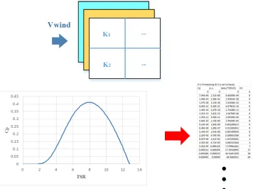
wind speed. To reduce the calculation load, both K1 and K2 are calculated off-line and then
stored in the parameter table of the PIC24. If it occurs when the measured wind speed does not match the lookup index, either roundup or interpolation can be made depending on the precision requirement and the memory size of the selected microprocessor. For here, the rounding method is firstly adopted. Following Eq. 2.10,cp is still needed to calculate the torque reference, which forms the second table, with λ as the look-up index. Again, this parameter table is expected to be obtained from either the turbine manufacturers or by certain aerodynamic modeling. This dissertation fits the second case, and the modeling and required cp table comes from Matlab/Simulink modeling and data post-processing. The studied characteristic is discussed at section 2.2, and the two tables are referred as Fig. 2.23. The design flowchart is shown in Fig. 2.24.
The digital implementation involves discretion and per unit conversion considering the low cost fixed-point processor. TSR λp.u. is modified to
λp.u.=
rωmωb
vwωbλb =k1
ωm
ωb
(2.8)
where
k1= rωb
vwλb
(2.9)
Turbine torque is converted accordingly as
Twtp.u.=
π
2r
2ρv3
w
Cpb
ωbTb
Cp
Cpb
ωbTb
ωm
=k2 Cpωb Cpbωm
(2.10)
where
k2 = π 2r
2ρv3
w
Cpb
ωbTb
2.5.2 Test Results
Figure 2.25: Implementation diagram of WTE.
Figure 2.26: WTE prototyping test setup.
Figure 2.28: Wind turbine emulator operation waveforms: dc bus voltage, PMSG Phase-A current, circulating dc current and speed feedback (from up to bottom).
Figure 2.30: Wind turbine emulator operation waveforms: dc bus voltage, IM three-phase currents (zoom in, from up to bottom).
2.6
Implementation and Test of the PMSG Rectifier System
This section discusses the hardware implementation and test of the PMSG rectifier system. The system controller function layout is shown in Fig. 2.32, where DSP TMS320F28335 is the main controller, and external analog to digital (AD) conversion is adopted, with up to 16 bits precision and ±10 V voltage range. Similarly, digital to analog (DA) conversion circuit is customized for debugging purpose[59]. Besides, as shown in Fig. 2.33, this PMSG rectifier system serves as one distributed renewable energy resource (DRER) node for Future Renewable Electric Energy Deliverable and Management (FREEDM) systems center, and thus the design also takes the communication functions into consideration. This is implemented through FPGA (Xilinx XC3S400) and one ARM board (TS-7800) with PC104 protocol. The ARM then communicate with the center SCADA system through DNP 3.0 communication protocol. The controller hardware is shown in Fig. 2.34, which includes interface conditioning board, control board, and ARM communication board. Fig. 2.35 shows the complete stack-structure based generator rectifier system. The power stage is acquired from Applied Power Systems, which can provide three-phase current and dc link voltage sensing for control applications. The machine position feedback is implemented with an incremental speed encoder acquired from BEI (1024 PPM), and the test waveforms are shown in Figs. 2.36 and 2.37. Fig. 2.38 shows the position angle with respect to the generator back EMF (open circuit). The space-vector modulation scheme is adopted for the PWM gating signals as seen in Figs. 2.39 and 2.40. The rectifier system operation at 200 rpm and constant torque mode is shown in Fig. 2.41, with roughly 280 W generation. And Fig. 2.42 shows a variable wind speed input scenario, where the drive is programmed at a jogging speed mode, and the generator is controlled under torque mode.
2.7
Conclusion
Figure 2.32: Layout of the WECS controller board.
Figure 2.34: Control system hardware components: (a) Interface conditioning board, (b) Con-trol board, (c) ARM board.
Figure 2.36: Encoder signal (AB).
Figure 2.37: Encoder index signal with position synchronization.
Figure 2.39: Space vector PWM gating signals (three bottom switch).
Figure 2.41: System operation waveforms at 200 rpm. Vdc= 380V, Pdc=280 W
Chapter 3
PI Passivity-based Control for
PMSG Wind Energy Conversion
System
3.1
Introduction
has been argued in [10] that nonlinear control designs may exhibit better performances. Classi-cal back-stepping methods have been used in [19, 20, 37], while [11] and [5] propose well known fuzzy and gain–scheduling controllers, respectively. Standard nonlinear control methods [30], based on feedback linearization, have been used in [9]. As mentioned above, all these works focus on the turbine control, making the assumption that the faster electrical part is ideally controlled by means of an inner loop whose references are provided by an outer loop involving the mechanical part. Therefore, there is no guarantee that the overall system will perform well or even preserve stability.
Controllers considering the whole system have also been reported. For example, [8] presented a sliding mode control of a wind system based on a fully actuated—hence, easier to control— doubly–fed induction generator. In [39], control of a solar and wind generation system to satisfy a power demand is accomplished using sliding mode control. By canceling undesirable nonlin-earities, the high-gain control renders the system passive respect to an energy function which depends on the sliding surface. In [48] is presented a control of a variable speed wind turbine emulator with a Permanent Magnet Synchronous Generator (PMSG) employing standard PI controllers with partial nonlinearity decoupling. As shown in [18], these PI controllers, generally without stability guarantee, are difficult to tune and exhibit poor robustness properties.
PMSG WECS is conducted [54]. The PBC method in this chapter follows the line of [27, 31, 67], where the final objective is to design a simple linear PI with guaranteed stability properties. Towards this end, a passive output for the nonlinear incremental model is identified, around which the stabilizing PI is added. The motivation of this work is to provide the guidelines for the design methodology of PI-PBC for the investigated WECS and verify its feasibility and advantages for such applications. The contributed comparison results of the PI-PBC and standard PI at the implementation level is provided.
One of the control objectives for variable speed wind turbines is to maximize the power capture from the wind. To carry out such a task, the turbine angular velocity is regulated by means of the electrical torque of the generator. Standard PI control structure is widely accepted in practice as they are easier to tune and simpler to implement than other existing model–based methods. Distinctive from the classical plant-controller picture, the passivity based controller is interconnected with other parts of the system and shapes the overall system energy function. The proposed PI-PBC is a linear PI controller, based on passivity, and the stability of the closed-loop system is guaranteed under practically reasonable assumptions.
Notation:Unless indicated otherwise, all vectors in the paper are column vectors. For a scalar functionH:Rn→R, we define∇xH:= ∂H∂x
>
—when clear from the context the subindex in
∇will be omitted.
3.2
System Modeling
3.2.1 Wind Turbine
The mechanical power extracted from the wind is given by the power function
Pw = 1
2ρACp(λ)v
3
w (3.1)
where vw is the wind speed, which is assumed constant and known,ρ is the air density, A is the area swept by the blades and Cp is the turbine’s coefficient power, which is function of the tip-speed ratio λdefined as
λ:= rωm
vw
, (3.2)
whereωm is the shaft’s rotational speed, andr is the blade’s radius.
The turbine’s power coefficient also depends on the blade pitch angle, and its functions have been discussed in previous chapters. In this chapter, we are interested in the operation regime where this angle is kept constant, also known as Region 2 [44]. For this reason this variable was omitted in the definition.
Fig. 3.2 shows a typical shape of the function Cp character. In the present approach, the generator rotational speed will be controlled to achieve the maximum power extraction, namely the system is required to operate in the point
λ?= arg maxCp(λ). (3.3)
This turbine character is assumed to be known beforehand from either test or the wind tur-bine manufacture, thusλ? is known. Consequently, the control task is to regulate the generator rotational speed at
ωm?:=
vwλ?
Figure 3.1: System under consideration
C
p(
λ
)
λ
Cp⋆
λ⋆
The dynamic equation of a wind turbine is obtained from Newton’s equation of motion
Jω˙m=−f ωm+Tm−Te (3.5)
whereJ is the rotor inertia, f >0 is a friction coefficient, Tm is the mechanical torque applied to the windmill shaft
Tm=
Pw
ωm = 1
2ρArv
2
w
Cp(λ)
λ , (3.6)
and Te is the electrical torque provided by the generator.
3.2.2 Permanent Magnet Synchronous Generator The dynamic equations of the generator in dq-coordinates are
L˙id=−Rid+Liqωe−vd
Li˙q=−Riq−Lidωe+φωe−vq
(3.7)
whereiq, id, vq, vdare respectively the q anddcomponents of the current and voltage,Rand L are the stator resistance and inductance respectively, φis the permanent magnetic flux andωe is the electrical frequency. The electrical frequency satisfies the relation
ωe=
P
2ωm. (3.8)
whereP is the number of pole pairs. The electrical torqueTe is given by
Te= 3 2
P
2φiq. (3.9)
The input voltages in the generator are
where d1 and d2 are duty ratio of the rectifier control signals in dq-coordinates. Finally, from
Kirchhoff’s current law we have
Cv˙C =−RevC+
VS
RS
+idd1+iqd2 (3.11)
where C is the capacitance value, Re := RRL+RS
LRS , RL is a resistive load and RS and VS are,
respectively, the supply internal resistance and dc voltage.
3.2.3 The Overall System
Substituting (3.6) and (3.9) in (3.5), (3.10) and (3.8) in (3.7) and from (3.11), the overall system becomes
Li˙d=−Rid+
P
2Liqωm−d1vC
Li˙q=−Riq−
P
2Lidωm+
P
2φωm−d2vC
Jω˙m=−f ωm+ 1 2ρAv 3 m 1 ωm Cp
vwωm
r
−3
2
P
2φiq
Cv˙C =−RevC +
VS
RS
+d1id+d2iq
Introducing the following definitions
φ1 := φP
2 , γ:=
P
2, J1 := 2
3J, f1 := 2
3f, (3.12)
and the change of variables
where the col() denotes the column of expressed vectors. The system can be rewritten as
˙
x1=−R
Lx1+ γ
J1x2x3− x4
Cu1 (3.14)
˙
x2=− γ J1
x1x3− R Lx2+
φ1 J1
x3− x4
Cu2 (3.15)
˙
x3=−f1x3+ Φ(x3)−φ1
Lx2 (3.16)
˙
x4=− Re
C x4+ x1
Lu1+ x2
Lu2+ VS
RS
(3.17)
where
Φ(x3) :=
1 3ρAJ1v
3
w 1
x3Cp
rx3 J1vw
.
Now, notice that the system admits the port–Hamiltonian representation [57]
˙
x= (J0(x3)− R+J1u1+J2u2)∇H(x) +E0(x3) (3.18)
where
H(x) := 1 2x
>Qx,
is the total energy of the system and the external force is defined as
E0(x3) := col
0,0,Φ(x3), VS
RS
and the matrices
Q:= diag
1 L, 1 L, 1 J1, 1 C ,
E0(x3) := col
0,0,Φ(x3),VS RS
,
R:= diag{R, R, f1, Re}>0,
J0(x3) :=
0 Jγ
1Lx3 0 0
−Jγ
1Lx3 0 φ1 0
0 −φ1 0 0
0 0 0 0
,
J1:=
0 0 0 −1
0 0 0 0
0 0 0 0
1 0 0 0
, J2:=
0 0 0 0
0 0 0 −1
0 0 0 0
0 1 0 0
.
3.2.4 Control Objectives as Desired Equilibrium Points
The control objectives are: 1) Minimize the copper loss and maximize the efficiency of the generator, this is carried out wheneverx1? = 0; 2) Operate at the maximum power extraction point x3? := J1λr?vw.
Lemma 1 The assignable equilibrium points of the system (3.14)-(3.17), compatible with the control objectives, are defined by the set
E=
x|x1= 0, x2=
L φ1
(Φ?−f1x3?), x3=x3?, h1(x4) = 0
where Φ?:= Φ(x3?)and
h1(x4) :=
Re
C2x 2 4−
VS
RSC
x4+
R φ2 1
(Φ?−f1x3?)2+
f1
J2 1
x23?−x3?
J1
Proof: At the equilibrium, (3.18) satisfies
0 = (J0(x3)− R)Qx+E0(x3) +G(x)u, (3.19)
where we defined the input matrix of the system (3.18) as
G(x) :=
J1Qx | J2Qx
.
The full–rank left–annihilator ofG(x) is
G⊥(x) =
x>Q
e>3
,
wheree3 := col(0,0,1,0). Multiplying (3.19) by G⊥(x) yields
−x>QRQx+J1
1x3Φ(x3) + VS
RSCx4
−f1x3+ Φ(x3)−φ1 Lx2
= 0.
Then, fixingx1= 0 and x3 =x3?, we get from the second equation,x2 = φL1Φ?−f1x3? :=x2?. Substituting the last value in the first equation yields the expression forh1(x4).
Remark 1 The necessary and sufficient condition for the existence of the desired equilibrium point is
R
φ21(Φ?−f1x3?) 2+ f1
J12x 2 3?−
x3?
J1
Φ?≤
VS2
3.3
Control Design: The PI-PBC Approach
3.3.1 Control Assumptions and Objectives
The control objectives are: 1) Maximize the PMSG efficiency for the studied PMSG, which is enacted by choosingid?= 0; 2) Achieve MPPT operation to maximize the energy capture. This research work considers a fixed pitch wind turbine application. A wind turbine level control which considers of pitch angle dynamics and functions is addressed in other publications [23]. Since an ideal energy storage device is adopted at the rectifier output side, there will be no captured power limitation for the studied system. The studied wind turbine power coefficient characteristics can either be tested or informed from the manufacturer side, and hence the optimalλis known. The corresponding optimal operation velocityωm? can then be calculated following ωm? := vwrλ?. The wind turbine characteristic will be addressed in detail at the simulation results section.
3.3.2 Control Design
To proceed with the design of the PI–PBC, the usual assumption that the mechanical dynam-ics is much slower than the electrical one is made, which translates into the following standing assumption.
Assumption 1 The system dynamics is represented by
˙
x= (J − R+J1u1+J2u2)Qx+E. (3.20)
where we defined J :=J0(x3?) andE :=E0(x3?).
Notice that we assumex3to be constant only when it appears in the interconnection matrix
J0 and the external forceE0, but it remains a state variable in the overall dynamics. Interested
Lemma 2 (Passivity) The system (3.20)defines a passive mappingu˜7→ywith storage function
V(˜x) = 1 2x˜
>
Qx,˜ (3.21)
where (˜·) = (·)−(·)? and the passive output is defined as
y:=G>(x?)Qx.˜ (3.22)
Proof. First, we define the incremental system of (3.20) as
˙
x=(J − R)Qx+G(x)(u?+ ˜u) +E (3.23)
Notice that at the equilibrium point x=x?
(J − R)Qx?+G(x?)u?+E = 0.
It follows that
G(x?)u?=−(J − R)Qx?−E. (3.24)
Differentiating (3.21) yields
˙
V = ˜x>Q[(J − R)Qx+G(x)(u?+ ˜u) +E]
=−x˜>QRQx˜+ ˜x>Q(G(x)−G(x?))u?+ ˜x>QG(x?)˜u
where (3.24) was employed. The proof is conclude realizing that
G(x)−G(x?) =G(˜x),
and by the fact that
Then, using these identities, the derivative yields
˙
V =−x˜>QRQx˜+y>u˜≤y>u,˜ (3.25)
which completes the proof.
As is well known [42] passive systems can be stably controlled with a PI as indicated in the proposition below.
Proposition 1 (PI-PBC) Consider the system (3.20)in closed–loop with the PI controller
˙
z=−y
u=−Kpy+Kiz,
(3.26)
where y is given in (3.22) and the tuning gains verify Kp > 0 and Ki > 0. For all initial
conditions (x(0), z(0)) the trajectories of the closed-loop system are bounded and
lim
t→∞x˜(t) = 0. (3.27)
Proof. Notice that (3.26) can be expressed as
˙˜
z=−y
˜
u=−Kpy+Kiz,˜
(3.28)
wherez? :=Ki−1u?. Consider the Lyapunov function candidate
W(˜x,z˜) =V(˜x) +1 2z˜
>
Differentiating this function and using (3.25) and (3.28) yields
˙
W =−x˜>QRQx˜+y>u˜−z˜>Kiy
=−x˜>QRQx˜−y>Kpy
≤ −α|x˜|2,
where| · | is the Euclidean norm and
α:=λmin{QRQ}>0.
Boundedness of the trajectories follows from Lyapunov’s Direct Method. The proof is completed from La Salle’s Invariance Principle which implies (3.27).
Remark 2 The passive output used in the PI controller of Proposition 1 is
y = 1
LC
x1?x˜4−x˜1x4?
x2?x˜4−x˜2x4?
(3.29)
which in the original system coordinates becomes
y=
id?˜vC−˜idvC?
iq?˜vC−˜iqvC?
(3.30)
3.4
Simulation Results
The proposed control design is implemented with Matlab/Simulink. The studied wind turbine power coefficient is assumed to be given by [26]
Cp(λ) =c1
c2 λi
−c5
exp
−c6
λi
wherec1 = 0.5, c2= 116, c5 = 5,c6= 21 and
λi =
1
λ−0.035
−1
.
The maximum value is Cp?= 0.411 and λ?= 7.954.
The parameters of the system were taken from [18] and are shown in Table 3.1. To test the controller in a real scenario, the simulation setting was realized in a switching based model. The considered PMSG wind turbine rectifier system is shown in Fig. 3.1. A constant voltage source is adopted at the dc output terminal to set the constant dc bus condition, which is normally maintained by the back-end converter. Space vector pulse width modulation (SVPWM) was adopted to generate the gate signals in the rectifier switches.
The control implementation diagram is shown in Fig. 3.3, where the real time equilibrium set is calculated following various wind speed. Distinct from the vector control based method, no cascaded loop structure is observed. Andq–axis reference still carries the speed information which is acquired from equilibrium point calculation. The dc bus voltage is also maintained at the reference value through the control. The control design flowchart is shown in Fig. 3.4. The wind profile is shown 3.5. To verify the controller performance under variable speed conditions, the wind profile involves two step variations. As it can be noticed from the profiles ofiq andid currents, they present typical switching noise, which is maintained in small range. A relatively good transient performance is seen without any overshoot and oscillation.
3.5
Comparison Study
Figure 3.3: Block diagram of the control implementation
6 9 12
v
w
!
m s
"
22.5 sec
div
Figure 3.5: Wind speed profile.
Table 3.1: Wind system parameters
Item Value
Turbine
Inertia J = 7.856 kg·m2
Blades radius r = 1.84 m PMSG
Nominal Power Sn= 5 kVA
Poles P = 28
Synchronous resistance R= 0.3676 Ω Synchronous inductance L= 3.55 mH
Flux φ= 0.2867 Wb
Friction coefficient f = 3.035×10⁻⁴ N·m·s
Rectifier & Electrical Parameters
Capacitance C = 3.3 mF
System Load RL= 60 Ω
Power Supply Voltage VS =400 V Power Supply Resistance RS= 0.1 Ω
3.5.1 The PI Controller Design
The proposed PI controller is depicted in Fig. 3.7 [16]. The cascaded loop structure is adopted for the design, of which the out loop regulates the rotor velocity with its reference generated for the inner q axis current;d axis current reference is set to 0. The analytical representation of the vector control strategy is
dd= 1
vC
−P
2Liqωm+u1
(3.31)
dq= 1
vC
P
2 (φ+Lid)ωm+u2
Figure 3.7: Standard PI control diagram.
where
u1 =kp1(id?−id) +ki1z1 (3.33)
u2 =kp3[kp2(ωm?−ωm)−iq] +kp3ki2z2+ki3z3 (3.34)
˙
z1 =id?−id (3.35)
˙
z2 =ωm?−ωm (3.36)
˙
z3 =kp2(ωm?−ωm) +ki2z2−iq. (3.37)
Gains kps and kis are chosen such that the linearization of (3.14)-(3.17) in closed–loop with (3.31)-(3.32) around the equilibrium point is exponentially stable. This means that the linearized system
˙
δx=Aδx (3.38)
has a Hurwitz matrix A ∈ R7×7. The entries of matrix A are: a11 := −L1 (R+kp1), a15 :=
ki1
L, a22 := −
1
L(R+kp3), a23 := − kp2kp3
L , a26 := ki2kp3
L , a27 := ki3
L , a32 :=
3 2
P φ
2J, a331 := 1For a scalar functionf:
R→R, we define (Df)(x?) := ∂f∂x(x)
−fJ +21JρAv3
w
h
1
ωm?(DCp)(λ?)−
Cp
ω2
m?
i
, a41 := kCvp1C?id?, a42 := Cviq?C?(R+kp3)−P φ2Cωvm?C?, a43 :=
iq?
CvC?
kp2kp3−P φ2
, a44:=−RCe+Cviq2
C?
Riq−P2ωm?
, a45:=−kCvi1iC?d?, a46:=−ki2CvkpC?3iq?, a47:=
−ki3iq?
CvC?, a51:= −1, a63 := −1, a72 :=−1, a73 := −kp2, a76:= ki2 The rest of the entries are
zero.
3.5.2 Case Study
For both considered scenarios, the adopted control parameters are listed as following. For stan-dard PI method, the PI gains are selected such that the linearization is exponentially stable. The chosen values arekp1 =kp3 = 17.8,ki1 =ki3= 1.8×10³,kp2= 27 andki2 = 54. The
eigen-values of (3.38) are: eig ={−3×10³, −5×10³, −1×10²,−2×10, −2.1, −5×10³, −1×10²}. On the other hand, matrices Ki and Kp in the PI-PBC of (3.22) were selected as Kp =Ki = diag(0.8, 0.8).
In the first case, vw is set as 10 m/s. The comparison results of the two control methods are provided in Fig. 3.8. It is observed that both methods can achieve a good control performance and reach the same equilibrium points for corresponding wind speed situation. However, PI-PBC demonstrates a smooth transition into steady state compared with PI method considering of generator velocity and q axis current waveforms.
Second case considers the wind speed stepping from 10 m/s to 11 m/s to testify the con-troller performance. Moreover, the switching model is adopted to prove the concon-troller’s dynamic response and switching characters. Fig. 3.9 shows the transient performance comparison of the two control methods. The following observations are in order.
1. Tuning the gains in the PI-PBC is simpler compared to the PI. This is due to fact that, when using the PI-PBC, there is a explicit condition on gain matricesKi, Kp.
3. It is observed that the PI-PBC is capable of stabilizing the system within a wider region. This is clearly observed from the system transient performance. Besides, the PI-PBC is not sensitive to the initial voltage of the dc link capacitor. However, the PI method tend to oscillate without correct initial settings in the simulation.
4. Future work includes a comparative study of the controller robustness for the two methods. As it can be seen from (3.31)-(3.32), the compensator part of the conventional PI controller depends directly on the system parameters.
5. Incrementing the gain values on the PI-PBC does not produce a obvious increment in the response. As a matter of fact, this behavior can be explained involving the zero dynamics of the system but might also be studied from the linearizaton of the closed–loop.
Third case considers the wind speed ramping case as indicated in Fig. 3.10 for a switching based model. The main purpose of this case study is to compare the transient response and system converging performance. The same test condition is also applied to the PI based system, with the results presented in Fig. 3.11. As it is highlighted, the PI-PBC method has a relatively slow convergence issues for the wind generator velocity (ωm) compared with the classical PI method. Even it has the inherent stability guarantee for the controller design. However, a faster speed response can increase the wind energy utilization efficiency considering a variable wind speed MPPT scenario. Thus a fundamental analysis for this issue is thus carried out.
3.6
Zero Dynamics Analysis
Before stating a lemma, first note that the output of the system inx’s coordinates is simply
˜
y(˜x) = ˜y(x−x?) = 1
LC
x1?x4−x4?x1
x2?x4−x4?x2.
(3.39)
Figure 3.9: Control performance comparison with stepping wind speed. (a) Wind speed. (b)
Lemma 3 Consider the system (3.14)-(3.17). The system zero dynamics respect to the passive output (3.39)are
˙
x3= Φ(x3, vw)−
φ1 L
x2?
x4?
x4
˙
x4=− 1
LC
ReL2x24?+RC2x22?
Cx2
2?+Lx24?
x4+ Cx2?x4?
Cx2
2?+Lx24?
φ1 J1x3+
Lx2 4?
Cx2
2?+Lx24?
VS
RS
(3.40)
Proof: From (3.39),
y= 0 ⇐⇒ x1 = x1?
x4?
x4 = 0 ∧ x2= x2?
x4?
x4. (3.41)
Multiplying (3.17) by LCx4?
x2?, adding (3.15), and substituting in the resulting equationx1,x2 in
agreement with (3.41) yields
x2?
x4? + L
C x4?
x2?
˙
x4 =−
L C2
x4?
x2?
Re+
R L
x2?
x4?
x4+ φ1 J1
x3+ L C
x4?
x2?
VS
RS
(3.42)
On the other hand, substituting x2 from (3.41) in (3.16) yields
˙
x3 = Φ(x3, vw)−
φ1 L
x2?
x4?
x4 (3.43)
From (3.42)-(3.43) follows (3.40).
It can be seen that the linearisation of (3.40) is
˙
x34=
Φ0(x3)|x3=x3? −
φ1 L
x4?
x2?
φ1 J1
Cx2?x4?
Cx2?+Lx1? − 1
LC
ReL2x21?+RC2x22?
Cx2?+Lx4?
x34 (3.44)
where we rewrite functionCp(λ) =Cp(Jrx1v3w) as
Cp(x3) =
α1
J1vw
r
1
x3 −β1
−α2
exp
−α3
J1vw
r
1
x3 −β1
Then, the derivative of Φ is
Φ0(x3) =
J
1vw
r
1
x33
α1
J
1vw
r
1
x3
−β1
−α2
α3−α1
− 1
x23
α1
J
1vw
r
1
x3
−β1
−α2
α0
exp
−α3
J
1vw
rx3
−β1
(3.46)
with α0 := 13ρAJ1vw3 and α1, α2, α3, β1 are parameters of Cp(x3) rewritten in (3.45).
Using the parameters of the system in Table 3.1, it follows that α1 = 58, α2 = 2.5, β1 =
0.035, α3 = 21, r = 1.84, J1 = 5.237, ρ = 1.225 with a constant wind speed vw = 10 and
x1?= 0, x2? = 0.0365, x3? = 226.402, x4? = 1.3192. Substituting them in (3.44) yields
˙
x34=
−0.181 −40845.630 0.0197 −3033.2667
x34. (3.47)
The eigenvalues of (3.47) are −0.446, −3033.001. It is noted that the larger the eigenvalue is, the faster the convergence will be. This small value directly corresponds to the slow convergence rate ofωm. This analysis fundamentally explains why the motor speed converges slowly.
3.7
Improved PI-PBC Method
Iq reference, real value, and from the PI-PBC are also highlighted together for comparison to prove the feasibility of the improved method. During ramping stage, or variable wind speed input interval, the PI-PBC method shows a divergence Iq command, this also explains why such convergence issue exists.
Figure 3.12: Improved PI-PBC control diagram.
3.8
Experimental Verification of the Improved PI-PBC Method
To verify the improved PI-PBC performance, experimental test is carried out. The hardware setup is shown in Fig. 2.26. For this test, the dc link is maintained with the power supply and paralleled load bank is adopted. The induction motor is controlled at torque mode. The PMSG is regulating the shaft speed. And in the following test results, the speed feedback, position angle,
state with load torque. At this interval, the speed is settled at 200 rpm with a phase current of 6.5 A (RMS). Fig. 3.16 shows system performance during the load step transient. Initially, system is settled under no load condition, which is indicated from the generatorq−axis current and the induction motor current, which is proportionally to the torque output. When the torque load added, the generatorq−axis current goes through a sudden dip, into negative value, which represents the generation condition. And the system can reach the steady state within less two seconds. Acceptable speed overshoot is observed, which is almost the same compared with above simulation results. Similar tests with higher PI gains are recorded in Fig. 3.17, where the speed overshoot becomes higher, and the position angle feedback is shown. Fig. 3.18 demonstrates the generator system transition from load condition to no load condition. 100 rpm is the current speed command, and during the load reduction transient, the generator goes over one cycle reverse rotation and quickly come back to the reference point. Fig. 3.19 shows the Iq and the generator speed performance. These tests prove that the system can handle the load step change and maintains a fast dynamic response. Fig. 3.20 and Fig. 3.21 present the torque load increase and decrease scenarios, respectively, of which the speed controller demonstrates satisfactory performance. Fig. 3.22 show the system speed generator speed regulation performance during loaded condition. The speed ramp (300 rpm to 100 rpm) is set in the PMSG controller, which is seen from the speed feedback DA results. During this transient, the generator current Iq is well maintained following the torque load. And Fig. 3.23 shows similar scenario, with the speed ramps from 100 rpm to 300 rpm.
3.9
Conclusion
Figure 3.14: Waveforms at no load startup.
Figure 3.16: Load torque step waveforms 1.
Figure 3.18: Load torque step waveforms 3.
Figure 3.20: System performance waveforms under load torque increase.
Figure 3.22: System operation waveforms under speed ramping 1.
![Figure 1.4:Basic configuration of a grid-connected wind turbine generation system [62].](https://thumb-us.123doks.com/thumbv2/123dok_us/1305357.1163176/20.612.91.541.101.397/figure-basic-conguration-grid-connected-wind-turbine-generation.webp)
![Figure 1.7:Type III: DFIG WECS [62].](https://thumb-us.123doks.com/thumbv2/123dok_us/1305357.1163176/22.612.133.496.382.592/figure-type-iii-dfig-wecs.webp)