in Database Management Systems
Rong Huang1, Rada Chirkova2, and Yahya Fathi1 1
Operations Research Program, NC State University Raleigh, NC 27695,
{rhuang,fathi}@ncsu.edu
2 Computer Science Department, NC State University, Raleigh, NC 27695,
Abstract. We present a study of the two-stage stochastic view selection problem in database management systems. The objective is to minimize processing times of the given queries subject to a storage limit. We as-sume that the queries are given in two or more workloads. We propose a two-stage stochastic programming (SP) model for this problem and study the structure and properties of its extensive form, which is an integer pro-gramming (IP) model. We use these properties to remove variables and constraints from this IP model, and obtain a smaller model with the same optimal solution. This allows us to solve realistic-size instances of the problem using commercial IP solvers. Subsequently, we present ap-propriate models, and techniques to assess the value of using a two-stage SP model, and discuss the value of perfect information. We discuss the properties of these values by conducting a computational experiment.
Keywords: Database management systems, View selection, Stochastic programming, Integer programming, Value of two-stage versus one-stage, value of stochastic solution, value of perfect information
1
Introduction
As an illustration, consider the following scenario. Large retailer companies (such as Sears, Kmart, Target, and WalMart in the USA) all maintain significant-size databases storing information about ongoing sales transactions. For instance, WalMart is known for maintaining database relations whose size is in billions of rows, ortuples. All these companies generally have significant volumes of mar-keting analysis going on throughout the year. That is, for accounting, reporting, and business-intelligence purposes, each company’s database system undergoes periodic runs of data-analysis queries on the stored information, including the queries for automatically or manually generated daily, weekly, or monthly sum-mary reports. In typical data-analysis, orOLAP (see [10] and [5]), queries, users are interested in obtaining summary information of a measure as a function of some business aspects, calleddimensions. For instance, in a daily volume-of-sales query in analyses run for Sears, the dimensions could beitem sold,date and time of sale, andcustomer.
Suppose the Sears sales data are stored in relations Sales, Time, and Customer. Suppose also that these relations form a star schema, with Sales as the “fact table” and Time and Customer as “dimension tables” (see [10]. Then the volume-of-sales query for November, 2010 could be expressed in the relational language SQL as the following grouping and aggregation over the star-schema join:
Q: SELECT itemCategory, customerType, sum(amount)
FROM Sales NATURAL JOIN Time NATURAL JOIN Customer WHERE dateMonth = 11 AND dateYear = 2010
GROUP BY itemCategory, customerType;
A data-management system evaluating the query Q on just the base relations would need to access all the sales information, including the likely large amount of irrelevant data for the salesbefore the reporting period. On the other hand, using derived data could reduce, perhaps significantly, the time to evaluate the queryQ. For instance, using anindex Ithat provides access to all sales events for all sales IDs for a specific month and year would obviate the need to access the irrelevant data for sales in months before (or after) November 2010. Note that evaluating the queryQusing the indexIwould still involve examining sales data at the granularity of individual sales events. Alternatively, the data-management system could reduce the evaluation time of the query Qby using amaterialized view V, which stores total sales per item category per customer type per month per year and is expressed in the relational language SQL as follows.
V: SELECT itemCategory, customerType, dateMonth, dateYear, sum(amount) FROM Sales NATURAL JOIN Time NATURAL JOIN Customer
GROUP BY itemCategory, customerType, dateMonth, dateYear;
time of Q when using V could be dramatically shorter than when not using V. Note also that the representation of the base data in the materialized viewVno longer distinguishes between individual items or sales dates.
Naturally in such a setting the problem of selecting an appropriate collection of derived data has to be addressed in the context of the objectives and lim-itations of that setting. In recent years several researchers have addressed the subject and developed exact and inexact methods for solving the problem in a one-stage deterministic environment, that is, where all queries are assumed to be known and given in advance, and a one-stage probabilistic environment, that is, where we have a probability of occurrence associated with each query in a given collection of queries. See [1], [2], [3], [6], [7], among others. [YF: give addi-tional references and update current refs]. In this article we study this problem in a two-stage environment and propose appropriate models and algorithms for solving the problem.
To illustrate this environment, let us refer to the Sears example described above. While some data-analysis queries would be posed on Sears’ sales data throughout the year, some of the queries may be run only at certain times of the year. The focus of such seasonally relevant queries could include, for instance: (i) demand for fancy gadgets (such as large-screen TVs) during heavy sales events (such as Black Friday in the USA); (ii) sales of deeply discounted basic household appliances during Christmas sale events; and (iii) August sale events for summertime gear. In such a situation, aside from designing and using derived data to improve the processing performance of the routine queries occurring throughout the year, it would be beneficial to design and use additional derived data in order to reduce the execution time of such seasonal queries as well. Of course it is natural that sometimes the collection of derived data that is useful for the queries in one season may be different from those that are useful for the queries in the subsequent seasons. On the other hand, it is always desirable if (at least some of) the derived data that is developed for one season can also be used for the queries in the subsequent seasons, since it would save both time and resources. After all, creating derived data itself requires both human and computational resources, and any savings in this regard translates to more efficiency in the overall operation. Hence, the problem in this context would be to determine the collection of derived data for two or more seasons (stages) so as to answer all the queries in an efficient manner while keeping the total volume of derived data as low as possible. In other words, in this context we need to propose two or more collections of interrelated derived data so as to minimize the overall query response time subject to a storage limit on the amount of derived data produced.
associated with each set. This, in turn, leads to a situation where we need to carry out the above mentioned analysis in a probabilistic environment, where we account for various scenarios (that is, query sets) that may occur in the future. For instance, in a situation where we deal with only two seasons, we may need to propose a collection of derived data to answer a given set of queries immediately (first season, or first-stage, queries), and a plan for several collec-tions of derived data, each collection associated with a possible set of future queries (second season, or second-stage, queries). In such a situation, in order to facilitate and expedite the process of creating the second-stage collections of derived data, it is clear that our decision for the first collection of derived data (that is, the first-stage decision) should be made with a view and consideration for various possibilities (queries) that may occur in the second stage. The idea here is to re-use in the second stage as many of the first-stage derived data as possible. This leads us to define and address a two-stage stochastic view selection problem as described in this paper.
Our specific contributions are as follows:
1. We define the two-stage stochastic view selection problem and model this problem as a two-stage stochastic programming (SP) model.
2. We study the structure and properties of the extensive form of the SP model, which is an integer programming (IP) model. We develop an algorithm that effectively reduces the search spaces of potentially beneficial views in the IP model, and obtain a smaller IP model whose solution is guaranteed to be optimal of the original SP model.
3. We conduct a computational experiment on the above IP models and dis-cuss the scalability of the reduced IP model. The reduced search spaces significantly reduce the size of our original IP model, so that for realistic-size instances of the problem this IP model can be solved efficiently by a commercial IP solver such as CPLEX [9].
4. We compare our two-stage SP model with several appropriate models and present techniques to assess the value of the SP model and the value of perfect information in this context.
5. We discuss the impact of the replacement mechanism on the optimal solu-tions in our SP model by conducting a sensitivity analysis.
2
The two-stage stochastic view selection problem
In this section, we first define the scope of the two-stage stochastic view selec-tion problem that we consider, i.e., the type of the database, queries and views. Subsequently, we propose a stochastic programming (SP) model [4] for this prob-lem. By studying the properties of the SP model, we then rewrite it as a model with fewer variables and constraints, and the resulting model is equivalent to the original SP model.
2.1 Formulation of the problem SVS
We consider a star-schema data warehouse (see [10] and [5]) with a single fact table and several dimension tables. In this context, we consider the evaluation cost of answering queries using unindexed materialized views such that each query can be evaluated using just one view and no other data. A queryqcan be answered using a viewv only if the set of grouping attributes ofv is a superset of the set of attributes in theGROUP BYclause ofqand of those attributes in the WHEREclause ofqthat are compared with constants. We usev to represent both a view and the collection of grouping attributes for that view, and we useq to represent both a query and the collection of attributes in theGROUP BY clause of that query plus those attributes in the WHERE clause of the query that are compared with constants. It follows that query qcan be answered by view v if and only if q⊆v. In order to evaluate a query using a given view (if this view can indeed be used to answer the query) we have to scan all rows of the view. Hence the corresponding evaluation cost is equal to the size of the view itself. We use ai to denote the size of each viewvi. We also use the parameterdij to denote the evaluation cost of answering queryqj using view vi. It follows that for each queryqj we have dij =ai ifqj ⊆vi, and we setdij= +∞otherwise.
In this environment we have a query workloadQ1 that we must answer at the present time (stage 1), and a second query workload Q2 that occurs at a future point in time (stage 2). We assume that the query workloadQ1 is known and given, but that the second query workloadQ2is a random set with a given probability distribution function. (We use boldface to emphasize that Q2 is a random set and differentiate it from a deterministic set such asQ1.) We illustrate all of these notions in Example 1 later in this subsection.
the views that we replace must not exceed a given storage limit b2. Naturally, b2≤b1.
In this context the technical problem that we need to address prior to stage 1 is to select all views in the setS1and a replacement plan associated with each possible realization Q2 ofQ2. The objective is to minimize the total evaluation cost for the queries at stage 1 plus the expected total evaluation cost for the queries at stage 2. Note that in order to obtain a global optimal solution for this problem which we callStochasticViewSelection(SVS) problem, all decisions regarding both stages (that is, the view set S1 and the replacement plan for every possible realizationQ2ofQ2) must be made prior to stage 1.
To illustrate, we present the following numeric example for a data cube [7] with 4 attributes.
Example 1. Given a database with four attributesa,b,c andd, the view lattice defined in [7] is shown in Figure 1. In this lattice, each node represents a view, and a directed edge from node v1 to nodev2 implies thatv1 is a parent of v2, that is,v2 can be obtained fromv1by aggregating over one attribute ofv1. The space requirement for each view in the lattice is given next to its corresponding node. In this instance, we assume that at stage 1, we are given two queries q1={a, b}andq2={b, c}. At stage 2,q3={b}andq4={a, c}would occur with probability 0.5, whileq5={c}andq6={b, d}would occur with probability 0.5. Equivalently,Q1={{a, b},{b, c}}, Q12 =
{
{b},{a, c}}, andQ22=
{
{c},{b, d}}. Assume the total space limitb1= 30 and the space limitb2= 15. Our objective is to minimize the cost of answering Q1 plus half of the cost of answering Q12 plus half of the cost of answeringQ2
2. We need to determine a collection of views S1 to materialize at stage 1, with the total size less than or equal to 30, and for each scenario at stage 2, we need to determine a subset ofS1to keep from stage 1 to stage 2, and another set of views to materialize at stage 2, with the total size less than or equal to 15.
2.2 A mathematical programming model
In this subsection, we describe a stochastic programming model for the above two-stage stochastic view selection (SVS) problem. Although the general form of the model that we propose is valid for any probability distribution function for Q2, in the following model and throughout the rest of this article we assumeQ2 is a random query set with Lpossible values. More specifically, we assume Q2 equals to query setQℓ
2 with probabilitypℓ, forℓ= 1 toL, where
∑L ℓ=1p
ℓ = 1. And we refer to each collection of queriesQℓ
2as ascenario. We start by defining the decision variables. For the first stage we define the following decision variables for all viewsvi∈V (whereV is the set of all views) and for all queriesqj∈Q1. xi=
{
1 if viewvi is materialized at stage 1 0 otherwise
zij =
{
Fig. 1.Lattice example with view sizes
For the second stage we define the following decision variables for all views vi ∈V, and for all queriesqj∈Qℓ2, forℓ= 1 toL.
uℓ i =
{
1 if viewvi is materialized at stage 1 and used in stage 2 for query setQℓ2 0 otherwise
yiℓ=
{
1 if view vi is materialized at stage 2 for query setQℓ2 0 otherwise
tℓ ij=
{
1 if we use viewvi to answer queryqj at stage 2 for query setQℓ2 0 otherwise
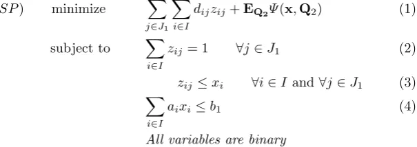
The cardinality of the view setV is 2K, where K is the number of distinct attributes in the database. Let I ={1,2, . . . ,2K} be the set of subscripts for all the views vi ∈ V. Also let J1 be the set of subscripts for all the queries qj ∈ Q1, and let J2ℓ be the set of subscripts for all the queries qj ∈ Qℓ2, for ℓ = 1,2, . . . , L. The problem can now be written as the following stochastic programming model [4] that we denote bySP.
(SP) minimize ∑
j∈J1
∑
i∈I
dijzij+EQ2Ψ(x,Q2) (1)
subject to ∑
i∈I
zij = 1 ∀j ∈J1 (2) zij ≤xi ∀i∈Iand ∀j∈J1 (3)
∑
i∈I
aixi≤b1 (4)
All variables are binary
where Ψ(x, Q2) is the minimum response time for a given set of values of the first stage variablesx=(x1,· · ·, x|V|
)
queries Q2, andEQ2 denotes mathematical expectation with respect toQ2. If
the probability distribution ofQ2is as discussed above, we have that
EQ2Ψ(x,Q2) = L
∑
ℓ=1
pℓΨ(x, Qℓ2) (5)
and for each value ofℓ, the corresponding value ofΨ(x, Qℓ
2) is obtained by solving the following view selection problem.
Ψ(x, Qℓ2) = min∑ j∈Jℓ 2
∑
i∈I
dijtℓij (6)
subject to ∑
i∈I
tℓij= 1 ∀j∈J2ℓ (7)
tℓij≤uℓi+yiℓ ∀i∈I and ∀j∈J2ℓ (8) uℓi ≤xi ∀i∈I (9)
∑
i∈I
aiyiℓ≤b2 (10)
∑
i∈I
ai(uℓi+yiℓ)≤b1 (11)
All variables are binary (12) Constraints (2) and (7) state that each query is answered by exactly one view in the set of materialized views. Constraints (3) and (8) guarantee that a query can be answered by a view only if the view is already materialized. Constraints (4), (10), and (11) state the storage limitation of view sets. Constraint (9) guarantees that the view kept from stage 1 to stage 2 is already materialized at stage 1.
In defining various decision variables in the above model we have used the subscript ito represent viewvi, and in every case we have defined the decision variables for all values of i in the subscript set I (or equivalently for all views in the entire view set V). Naturally, in practice for each decision variable with a subscript i(associated with view vi) we only need to consider those views vi that are relevant in the context of that decision variable. For instance, in defining the decision variablexi at stage 1 we only need to define this variable for those viewsvithat can be used to answer at least one query either in the first stage or in the second stage. In other words, we need not consider viewvi (or define the corresponding variablexi) if this view is not a superset of at least one query in our entire query set. In the remainder of this section we define various subsets of the overall view setV (and its corresponding subscript setI) so as to re-write the above model with few variables and constraints.
LetQb=Q1∪{∪L ℓ=1Qℓ2
}
be the collection of all queries (either in stage 1 or in stage 2). We define
V1=
{
vi∈V :vi⊇q for someq∈Qb
}
(13) V2ℓ={vi∈V :vi⊇qfor some q∈Qℓ2
}
Correspondingly, we define the sets of subscripts associated with V1 andV2ℓ as I1andI2ℓ, forℓ= 1 toL, respectively. It follows thatV1is the set of views that are relevant for stage 1, andVℓ
2 is the set of views that are relevant for the ℓth sub-problem (scenario) in stage 2, forℓ= 1 toL.
Similarly, associated with each queryqj in the setsQ1 and/orQℓ2 we define a sub-collection of views that are relevant in answering that particular query. For each queryqj ∈Q1 we defineV1j ={vi ∈V1:vi⊇qj}, and for each query qj∈Qℓ2we define V
ℓ 2j=
{
vi∈V2ℓ:vi⊇qj
}
, forℓ= 1 toL. Again, correspond-ing to the view sets V1j and V2ℓj we define the associated sets of subscripts as I1j andI2ℓj, forℓ= 1 toL, respectively.
Example 1 (Continued).In order to defineV1,V21 andV22, we only consider the views that could answer at least one query in the query setQb={q1, q2, q3, q4, q5, q6}, Q12 andQ22, respectively. Thus, we obtain that
V1=
{
{b},{c},{a, b},{a, c},{b, c},{b, d},{c, d},{a, b, c},{a, b, d},{a, c, d},
{b, c, d},{a, b, c, d}}
V21={{b},{a, b},{a, c},{b, c},{b, d},{a, b, c},{a, b, d},{a, c, d},{b, c, d},{a, b, c, d}} V22={{c},{a, c},{b, c},{b, d},{c, d},{a, b, c},{a, b, d},{a, c, d},{b, c, d},{a, b, c, d}}.
For each query, we define the relevant view sets in answering that particular query. For example, for queryq1={a, b} ∈Q1we defineV11=
{
{a, b},{a, b, c},
{a, b, d}, {a, b, c, d}}, and for query q6 ={b, d} ∈ Q22 we define V262 ={{b, d},
{a, b, d}, {b, c, d}, {a, b, c, d}}.
We can now define the first stage decision variablesxi, only for views in the set V1, and the first stage decision variables zij, only for views vi in the set V1j. Similarly, we can define the second stage decision variablesuℓ
i andyℓi, only for views vi ∈ V2ℓ, and the second stage decision variables t
ℓ
ij, only for views vi ∈V2ℓj, forℓ= 1 toL. It follows that we can now rewrite the above stochastic programming modelSP as the following model that we denote bySP′.
(SP′) minimize ∑
j∈J1
∑
i∈I1j
dijzij+EQ2Ψ(x,Q2) (15)
subject to ∑
i∈I1j
zij= 1 ∀j∈J1 (16)
zij≤xi ∀j∈J1 and∀i∈I1j (17)
∑
i∈I1
aixi≤b1 (18)
and the corresponding second stage subproblem can be written as
Ψ(x, Qℓ2) = min∑ j∈Jℓ 2
∑
i∈Iℓ 2j
dijtℓij (20)
subject to ∑
i∈Iℓ 2j
tℓij = 1 ∀j ∈J2ℓ (21)
tℓij≤uℓi+yℓi ∀j ∈J2ℓ and∀i∈I2ℓj (22) uℓi ≤xi ∀i∈I2ℓ (23)
∑
i∈Iℓ 2
aiyiℓ≤b2 (24)
∑
i∈Iℓ 2
ai(uℓi+yiℓ)≤b1 (25)
All variables are binary (26)
3
Solving the model
SP
We begin this section by introducing an integer programming model [16] ob-tained from the extensive form [4] of the above stochastic programming model. Later in this section we study the properties of the integer programming model, use these properties to remove some variables and constraints, and obtain a model that is significantly smaller. The optimal solution of the resulting model is guaranteed to be optimal for the original modelSP. This, in turn, allows us to solve larger instances of the SVS problem.
3.1 An integer programming model
(IP1) minimize ∑ j∈J1
∑
i∈I1j
dijzij+ L
∑
ℓ=1 pℓ
∑
j∈Jℓ 2
∑
i∈Iℓ 2j
dijtℓij (27)
subject to ∑ i∈I1j
zij= 1 ∀j∈J1 (28)
zij ≤xi ∀j∈J1,∀i∈I1j (29)
∑
i∈I1
aixi≤b1 (30)
∑
i∈Iℓ 2j
tℓij = 1 ∀j∈J2ℓ, ℓ= 1, . . . , L (31)
tijℓ ≤uℓi+yiℓ ∀j∈J2ℓ,∀i∈I2ℓj, ℓ= 1, . . . , L (32) uℓi ≤xi ∀i∈I2ℓ, ℓ= 1, . . . , L (33)
∑
i∈Iℓ 2
aiyiℓ≤b2, ℓ= 1, . . . , L (34)
∑
i∈Iℓ 2
ai(uℓi+y ℓ
i)≤b1, ℓ= 1, . . . , L (35)
All variables are binary (36) Note that for an instance withKattributes,n1 queries inQ1 at stage 1 and nℓ
2 queries inQℓ2at stage 2, forℓ= 1, . . . , L, there are at most (n1+
∑L ℓ=1n
ℓ 2+ 2L+ 1)|V1|variables and at most (n1+∑Lℓ=1nℓ
2+ 2L)(|V1|+ 1) + 1 constraints in the integer programming model IP1, where V1 is as defined in Section 2.2. Thus, even for a relatively small number ofK,L,n1 andn1
2,· · ·, nL2, the size of the model could be very large and the execution time of solving the IP model could be excessively long even with a relatively fast IP solver such as CPLEX 11 [9]. The applicability of our model is thus limited to only a small number of instances. We thus consider to reduce the size of our model by reducing the view setsV1,V1j,V2ℓandV2ℓj, forℓ= 1, . . . , L. In section 4, we will provide numerical results for solving modelIP1.
3.2 Reduction of search space
First reduction In a deterministic view selection problem, Asgharzadeh [1] proposes that one could reduce the search space of views (set of views to consider) by eliminating view v that has at least one attribute that is not in any of the queries answerable by this view. We extend the methods to our SVS problem and obtain the following observations.
Observation 1 In an instance of SVS problem, given a view vi in the view
set V1, if the number of attributes of vi is strictly greater than the number of
attributes in the union set of the queries inQbthatvicould answer, that is,|vi|>
| ∪q∈Qb q⊆vi
q|, then there exists an optimal solution such that vi is not materialized
at stage one, or equivalently,xi= 0.
Proof. For each query q∈Qb, if q could be answered byvi, thenq⊆vi. Thus,
∪q∈Qb q⊆vi
q ⊆vi and | ∪q∈Qb q⊆vi
q| ≤ |vi|. If | ∪q∈Qb q⊆vi
q| <|vi|, then vi has at least one attribute, call it attribute a, that is not in anyq∈Qb such thatq⊆vi. If there exists an optimal solution such that vi is materialized at stage one, we replace it with view v\ {a}. Since the size of vi\ {a} is no more than that of vi, the replacement will not violate the space limitation. And for each queryq∈Qbthat is answered byvi in the optimal solution,q could be answered byvi\ {a} with cost no more than that ofvi. Thus, we obtain an optimal solution such thatv is not materialized at stage one and the corresponding decision variablexi= 0. Observation 2 In an instance of SVS problem, given a view vi in the view
set Vℓ
2, if the number of attributes of vi is strictly greater than the number of
attributes in the union set of the queries inQl
2thatvicould answer, that is,|vi|>
| ∪q∈Qℓ2 q⊆vi
q|, then there exists an optimal solution such thatvi is not materialized
at stage two, or equivalently, yℓ i = 0.
Proof. Ifvisatisfies the above conditions, thenvi has at least one attribute, say attribute a, that is not in anyq ∈Qℓ
2 and q⊆v. Ifvi is materialized at stage two in an optimal solution, then replacevi byvi\ {a}and the solution remains optimal.
Second reduction In the deterministic view selection problem, Asgharzadeh, Chirkova, Fathi [2] and Asgharzadeh [1] propose that one could reduce the search space of views based on the size of the views and on the total size of the queries that each view could answer. LetS(·) be the size of a query or a view. Then, we obtain the following observations.
Observation 3 In an instance ofSV S problem, given a viewvi in the view set V1, if vi satisfies the condition that the size of vi is greater than the total size
of the queries in Qb that this view can answer, that is, S(vi)>
∑
q∈Q,qb ⊆viS(q),
then there exists an optimal solution in whichvi is not materialized at stage one,
Proof. Assume thatvi ∈V1satisfies the above inequality condition and that vi is materialized at stage one in an optimal solution. Note that a query could be answered by a view with the same set of attributes as the query, and the sizes of the query and the view are identical. LetV(v, Q) be the set of views that have the same set of attributes as the queries that a viewvcould answer in a query set Q. At stage 1, if we materialize all the views inV(vi,Qb) instead ofvi, then the space limitation is not violated because of the above inequality condition. And every query in Qb that vi answers could be answered by some view in V(vi,Qb) with cost no more thanS(vi). Thus, the new solution remains optimal.
Observation 4 In an instance of SVS problem, given a viewvi in the view set Vℓ
2, ifvi satisfies the condition that the size ofvi is greater than the total size of
the queries inQℓ
2 that this view can answer, that is, S(vi)>
∑
q∈Qℓ2 q⊆vi
S(q), then there exists an optimal solution such that vi is not materialized at stage two, or
equivalently,yℓ i = 0.
Proof. Ifvi∈Qℓ2 satisfies the above condition and is materialized at stage two in an optimal solution, then replace vi by the set of views V(vi, Qℓ2) and the solution remains optimal.
Note that the first and second reductions on the same set of views could be conducted simultaneously. It follows that we can now derive the reductions on the view setV1based on Observations 1 and 3, and derive the reductions on the view setVℓ
2 based on Observations 2 and 4. We denote the reduced view sets of V1 andVℓ
2 as V1 andV2ℓ, forℓ= 1 toL, respectively.
We further define a new set of views for each scenarioℓthat we refer to asVℓ 12. This would be the set of views that are materialized at stage 1 and potentially utilized for scenario ℓ at stage 2. In the following observation, we show that Vℓ
12=V1∩V ℓ 2.
Observation 5 For each viewvithat is materialized at stage one and kept from
stage one to stage two for the ℓth scenario, v
i∈V1∩V2ℓ.
Proof. The proof of Observation 5 is straightforward. Observation 6 Vℓ
2 ⊆V12ℓ ⊆V1, forℓ= 1, . . . , L.
Proof. Firstly, Vℓ
12 ⊆ V1 could be obtained directly from the definition of V12ℓ. Secondly, we show Vℓ
2 ⊆ V1. Noting that V2ℓ ⊆ V2ℓ ⊆ V1, we obtain that for all v ∈ Vℓ
2, v ∈ V1. Assume v ̸∈ V1. Then, v must be eliminated during first or second reduction. If v satisfies the first reduction condition, that is, |v| >
| ∪q∈Qb q⊆v
q|. Since Qℓ
2 ⊆ Qb, ∪q∈Qℓ2 q⊆v
q ⊆ ∪q∈Qb q⊆v
q. Thus, |v| > | ∪q∈Qℓ 2 q⊆v
q| and v is eliminated from Vℓ
2 by first reduction. And thus v ̸∈ V2ℓ. This contradicts the conditionv∈Vℓ
that is, S(v) > ∑q∈Qb q⊆v
S(q). Since Qℓ 2 ⊆ Qb,
∑
q∈Qb q⊆v
S(q) ≥ ∑q∈Qℓ 2 q⊆v
S(q). Thus, S(v)>∑q∈Qℓ
2 q⊆v
S(q) andv is eliminated fromV2ℓ by second reduction. And thus v̸∈Vl
2. This contradicts the condition v∈V2ℓ. Hence, the assumption does not hold andv∈V1, which proves thatVℓ
2 ⊆V1. Thirdly, sinceV2ℓ⊆V2ℓ, we obtain that Vl
2 ⊆V ℓ
2 ∩V1=V12ℓ.
Correspondingly, we define the sets of subscripts for V1, Vℓ
12 and V2ℓ as I1, Iℓ
12andI2ℓ, forℓ= 1 toL, respectively.
For each queryqj ∈Q1we defineV1j ={vi ∈V1:vi⊇qj}, and for each query qj ∈Qℓ2 we define V12ℓj = {vi ∈V12ℓ : vi ⊇qj} andV2ℓj ={vi ∈ V2ℓ : vi ⊇qj}, forℓ= 1 toL. It follows thatVℓ
2j⊆V12ℓj by Observation 6. Again, we define the associated sets of subscripts forV1j,V12j andV2ℓj as I1j,I12j andI2ℓj, forℓ= 1 toL, respectively.
Example 1 (Continued).View{c, d}in the setV1 answers only one query{c}in
b
Q, and contains one more attribute than{c}. As a result, view{c, d} is elimi-nated fromV1 by the first reduction. View{a, b, d}in the setV1 answers query
{b},{a, b}and{b, d}inQb, and the total size of the three queries is less than the size of view {a, b, d} (4 + 7 + 8 = 19<20). As a result, view {a, b, d} is elimi-nated from V1 by the second reduction. With the same approaches, we obtain the reduced view sets as follows.
V1={{b},{c},{a, b},{a, c},{b, c},{b, d},{a, b, c},{b, c, d},{a, b, c, d}} V1
12=
{
{b},{a, b},{a, c},{b, c},{b, d},{a, b, c},{b, c, d},{a, b, c, d}} V1
2 =
{
{b},{a, c},{a, b, c}} V2
12=
{
{c},{a, c},{b, c},{b, d},{a, b, c},{b, c, d},{a, b, c, d}} V2
2 =
{
{c},{b, d}}.
For each query, we define the relevant view sets in answering that particular query. For example, for queryq1={a, b} ∈Q1we defineV11=
{
{a, b},{a, b, c},
{a, b, c, d}}, and for query q6 ={b, d} ∈Q2
2, we define V12 62 =
{
{b, d}, {b, c, d},
{a, b, c, d}}andV2 26=
{ {b, d}}.
In Section 4, we will provide the numerical results of our reductions of the search space by a number of instances.
Modified integer programming model IP2 We can now redefine the first stage decision variablesxionly for views in the setV1, and the first stage decision variableszij only for viewsvi ∈V1j. Similarly, we can redefine the second stage decision variables uℓ
variablesyiℓonly for viewsvi∈V2ℓ. SinceV2ℓj⊆V12ℓj, we can redefine the second stage variablestℓ
ij only for viewsvi∈V12ℓj, forℓ= 1 toL. It follows that we can now rewrite the integer programming model IP1 into an integer programming model that we denote asIP2 with reduced size.
(IP2) minimize ∑ j∈J1
∑
i∈I1j
dijzij+ L
∑
ℓ=1 pℓ
∑
j∈Jℓ 2
∑
i∈Iℓ 12j
dijtℓij (37)
subject to ∑ i∈I1j
zij = 1 ∀j∈J1 (38)
zij ≤xi ∀j∈J1,∀i∈I1j (39)
∑
i∈I1
aixi≤b1 (40)
∑
i∈Iℓ 12j
tℓij= 1 ∀j∈J2ℓ, ℓ= 1, . . . , L (41)
tℓij ≤uℓi ∀j∈J2ℓ,∀i∈Iℓ 12j−I
ℓ
2j, ℓ= 1, . . . , L (42) tℓij ≤uℓi+yℓi ∀j∈J2ℓ,∀i∈Il
2j, ℓ= 1, . . . , L (43) uℓi≤xi ∀i∈I12ℓ , ℓ= 1, . . . , L (44)
∑
i∈Iℓ 2
aiyℓi ≤b2, ℓ= 1, . . . , L (45)
∑
i∈Iℓ 12
aiuℓi+
∑
i∈Iℓ 2
aiyiℓ≤b1, ℓ= 1, . . . , L (46)
All variables are binary (47) The optimal solution ofIP2 is also an optimal solution ofIP1. Thus, given an SVS problem, we could solve it by solvingIP2. SinceV1j,V12ℓj,V2ℓj,V12ℓ andV2ℓ are all subsets ofV1, we could obtain an upper bound (n1+∑Lℓ=1nℓ2+2L+1)|V1| for the number of variables and an upper bound (n1+
∑L ℓ=1n
ℓ
2+2L)(|V1|+1)+1 for the number of constraints in IP2. Compared with IP1, both numbers are dramatically reduced, and thus the size ofIP2 can be significantly smaller than IP1. In section 4, we will provide numerical results for the comparisons ofIP1 andIP2.
4
Experimental results of solving the SVS problem
construct a collection of instances of the SVS problem with varying sizes using a number of databases of the TPC-H benchmark [15]. We then solve each instance using models IP1 and IP2. We observe that the search spaces of views are significantly reduced in IP2 compared with IP1, which allows us to use IP2 to solve several larger instances of the SVS problem of realistic size. We also observe that some realistic-size instances could not be solved due to insufficient memory. We have implemented all of our algorithms in C++, and have used CPLEX 11 [9] to solve the integer programming modelsIP1 andIP2.
In Section 4.1 we describe how we construct each of the instances in our experiments. In Sections 4.2 and 4.3 we evaluate the effectiveness of our models for solving the SVS problem, and report our findings. Finally in Section 4.4 we present a summary of our experimental results.
4.1 Constructing instances
The input parameters for an instance of the SVS problem are a given database
D, query sets Q1 and Q2 = {Q12, . . . , QL2}, associated probability vector p = (p1, . . . , pL), and the space limitsb1 andb2. Thus, each instance is identified by (D, Q1,Q2,p, b1, b2).
In this section, all the instances are constructed based on three different databases of the TPC-H benchmark [15]. More specifically, we use a 7-attribute database, a 13-attribute database and a 17-attribute database to construct the collection of instances in our experiments. Each database was obtained by adding, to the original stored TPC-H tables generated with scale factor one, a single re-lation, with either 7, 13, or 17 grouping attributes, that results from the natural join of a subset of the set of these base relations. We measure the size of each view in terms of the number of bytes that it occupies, and estimate this value using analytical methods.
For all instances in this section, we setL= 2. Equivalently, there are 2 po-tential query sets,Q1
2andQ22, that occur at stage 2, with respective probabilities p1andp2. We further assume thatp1=p2= 0.5.
In order to construct query setsQ1,Q1
2andQ22for each instance, we comply with the following principles. In each query set, each query is generated over the given database randomly. In addition, the total sizes of all the query sets are “approximately” the same. More specifically, the difference between the sizes of any two query sets is no more than the size of the raw-data view.
Given a database fact table (that is, stored relation)DwithKattributes, in order to randomly choose a queryq, we first determine the number of attributes in qby randomly generating an integertfrom {1,2, . . . , K−1}. Then, we ran-domly chooset distinct integers a1, . . . , at from {1,2, . . . , K} as the attributes ofq. Then, {a1, . . . , at} uniquely defines queryqover databaseD.
To determine the queries in each query set, we first choose an integer n1, ranging from 20 to 50, as the number of queries in Q1. For some instances, we also set n1 to several larger values. Then, we randomly generaten1 queries over databaseD as query setQ1. In order to obtain query sets Q1
size of the generated queries is less than or equal toSize(Q1), but not less than Size(Q1)−Size(v1), where Size(·) denotes the total size of the queries in a query set (·), andv1 denotes the raw-data view. Thus, we obtain that
S(v1) +Size(Qℓ2)≥Size(Q1)≥Size(Qℓ2), ℓ= 1,2 (48) The difficulty of solving a specific instance of the SVS problem depends on the relative size of the storage spaces as compared with the size of the queries. Suppose the size of storage spaceb1is expressed as
b1=α·Size(Qb) (49) whereαis a non-negative real number andQb=Q1∪Q12∪Q22.
Ifb1 ≥S(v1), the problem is feasible, since we could always materialize the raw-data view and use it to answer all the queries. And if b1 < S(v1), there is no guarantee that the SVS problem is feasible.
Ifα≥1, the SVS problem becomes trivial, since the best solution could be materializing all the views with the same sets of attributes as the queries inQb at stage 1. Thus, in order for an instance of the SVS problem to be nontrivial, we need to have 0< α <1.
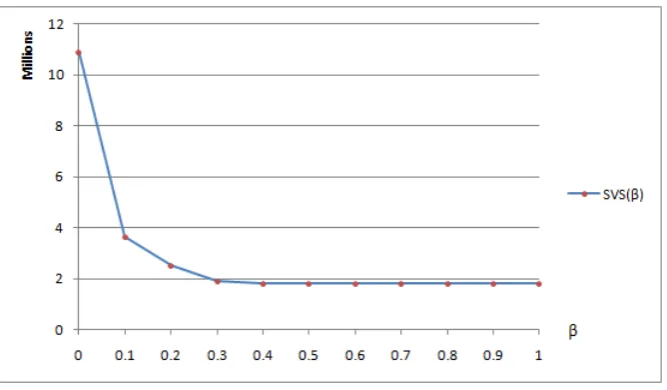
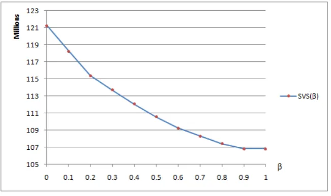
Note thatb2 ≤b1 always holds on the space limitsb1 andb2. Supposeb2 is expressed as
b2=βb1 (50) where 0≤β≤1.
Ifb2 ≥maxQ∈{Q1
2,...,QL2}Size(Q), the second stage sub-problem of the SVS problem becomes trivial, since at stage 2, for each scenarioℓwe can materialize all the views with the same set of attributes as the queries inQℓ
2.
In this section, for all instances based on the TPC-H datasets we choose α= 0.2 and β = 0.5, that is, the storage space limitb1 is equal to one-fifth of the sum of the sizes of the queries inQb, andb2 is one-half ofb1. It follows that
b1= 0.2Size(Qb)≤(0.2)(3Size(Q1)) = 0.6Size(Q1) b2= 0.5b1≤(0.5)(0.6Size(Q1))≤0.3Size(Q1)
which guarantees that the instances of the SVS problem are nontrivial.
4.2 Reducing the search space
Table 1.Comparison of search spaces in modelsIP1 andIP2, for instances over the 7-attribute TPC-H database
inst-ance
query sets (|Q1|,|Q12|,|Q22|)
number ofxinumber ofu1i number of yi1number ofu2i number ofy2i
IP1 IP2 IP1 IP2 IP1 IP2 IP1 IP2 IP1 IP2
|V1| |V1| |V21| |V12|1 |V 1
2| |V21| |V 2
2| |V12| |2 V 2 2| |V22|
1 (20,17,19) 125 64 80 54 80 24 108 55 108 43
2 (20,25,20) 125 84 122 82 122 47 110 75 110 38
3 (30,35,39) 127 105 124 102 124 65 120 99 120 62
4 (30,26,31) 127 92 120 88 120 42 124 89 124 58
5 (40,45,41) 127 109 122 104 122 72 123 105 123 77
6 (40,38,35) 126 103 120 98 120 62 116 99 116 44
7 (50,48,50) 127 119 121 113 121 91 126 118 126 85
8 (50,47,53) 127 113 124 110 124 74 125 111 125 87
Table 2.Comparison of sizes and computing times in models IP1 and IP2, for in-stances over the 7-attribute TPC-H database
inst-ance
query sets (|Q1|,|Q12|,|Q22|)
number of number of time to build time to solve variables constraints model (sec.) model (sec.)
IP1 IP2 IP1 IP2 IP1 IP2 IP1 IP2
1 (20,17,19) 1621 901 1425 873 0.015 0.000 0.734 0.469
2 (20,25,20) 1937 1315 1838 1288 0.015 0.000 1.500 1.235 3 (30,35,39) 2575 2135 2527 2076 0.000 0.016 0.938 0.859 4 (30,26,31) 2385 1761 2330 1738 0.000 0.015 8.312 6.969 5 (40,45,41) 2873 2523 2859 2456 0.015 0.016 6.297 5.640 6 (40,38,35) 2600 2139 2556 2139 0.015 0.016 2.031 1.859 7 (50,48,50) 3447 3209 3459 3122 0.016 0.015 8.156 6.110 8 (50,47,53) 3437 3060 3455 3001 0.015 0.015 3.125 1.625
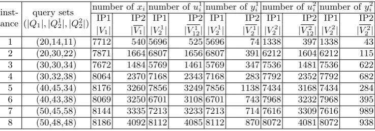
Table 3.Comparison of search spaces in modelsIP1 andIP2, for instances over the 13-attribute TPC-H database
inst-ance
query sets (|Q1|,|Q12|,|Q22|)
number ofxinumber ofu1i number of y 1
i number ofu 2
i number ofy 2 i
IP1 IP2 IP1 IP2 IP1 IP2 IP1 IP2 IP1 IP2
|V1| |V1| |V21| |V12| |1 V21| |V21| |V 2
2| |V12| |2 V22| |V22|
1 (20,14,11) 7712 540 5696 525 5696 74 1338 397 1338 43
2 (20,30,22) 7871 1664 6807 1656 6807 391 6212 1604 6212 115
3 (30,30,34) 7672 1484 5769 1461 5769 347 7536 1481 7536 622
4 (30,32,38) 8064 2370 7168 2343 7168 283 7792 2352 7792 682
5 (40,45,34) 8176 3260 7856 3249 7856 1138 7434 3168 7434 284
6 (40,43,38) 8069 3250 6701 3108 6701 743 7968 3232 7968 395
7 (50,45,58) 8144 3335 7213 3233 7213 714 7616 3309 7616 989
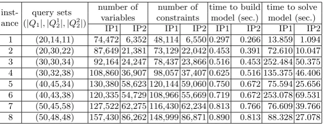
Table 4.Comparison of sizes and computing times in models IP1 and IP2, for in-stances over the 13-attribute TPC-H database
inst-ance
query sets (|Q1|,|Q12|,|Q22|)
number of number of time to build time to solve variables constraints model (sec.) model (sec.)
IP1 IP2 IP1 IP2 IP1 IP2 IP1 IP2
1 (20,14,11) 74,472 6,352 48,114 6,550 0.297 0.266 13.859 1.094
2 (20,30,22) 87,649 21,381 73,129 22,042 0.453 0.391 72.610 10.047 3 (30,30,34) 92,164 24,247 78,437 23,866 0.516 0.453 252.484 50.375 4 (30,32,38) 108,860 36,907 98,057 37,407 0.625 0.516 135.375 46.406 5 (40,45,34) 130,380 58,623 120,144 59,060 0.750 0.672 75.594 25.656 6 (40,43,38) 120,335 54,729 108,966 55,669 0.719 0.672 253.078 69.531 7 (50,45,58) 127,522 62,275 116,430 62,234 0.813 0.766 76.609 39.766 8 (50,48,48) 157,430 86,262 148,999 86,871 0.890 0.813 88.328 27.078
CPLEX IP solver, for models IP1 and IP2. The results are shown in Table 2 and Table 4.
We observe that the number of views in the search space for modelIP1 is significantly reduced inIP2 over all the instances. It is also observed that the size ofIP2, when expressed by the total number of variables and constraints, is much smaller than that ofIP1, yet the optimal solution ofIP2 is also optimal for the modelIP1. While there is no significant difference between the time to build the models IP1 and modelIP2, the time to solveIP2 is significantly smaller than that ofIP1, especially for relatively large problems, such as instances based on the 13-attribute database.
We observe that the reduction in the number of each group of decision vari-ables and the reduction in the size of the model, expressed by the reduction in the total number of variables and constraints, are relatively large for instances with a small ratio of the number of queries over the total number of views in the database. For instances with larger ratios, the reduction rate decreases. More specifically, we compare the results for instances over the 7-attribute database in Tables 1 and 2. When we increase the number of queries in each query set of the instances, the ratio of the number of queries over the total number of views increases, and the magnitude of associated reductions in the number of variables decreases. We also compare the results for the instances with similar number of queries based on different databases. More specifically, we compare each pair of instances with same instance ID over the 7-attribute database and the 13-attribute database. Note that the number of views in the 7-13-attribute database and in the 13-attribute database are 128 and 8192, respectively. For each pair of instances, the one over the 13-attribute database has a relatively small ratio of the number of queries over the total number of views, and the associated reductions are relatively large.
4.3 Scalability of the model IP2
In this subsection we evaluate the scalability of the modelIP2 to solve instances of the SVS problem. Based on the results in Tables 2 and 4, we could solve all the instances over the 7-attribute TPC-H database usingIP2 within 10 seconds, and all the instances over the 13-attribute TPC-H database within 80 seconds. In order to examine the scalability of model IP2, we construct instances with the number of queries in Q1 varying from 60 to 200 based on the 13-attribute TPC-H database, and instances with the number of queries inQ1varying from 20 to 40 based on the 17-attribute TPC-H database. We solved all the instances using modelIP2, and reported the time required to build the model and the time required to solve the model for the corresponding IP2 based on each instance. The results are shown in Table 5 and Table 6.
Table 5.Scalability ofIP2 for instances over the 13-attribute TPC-H database
instance query sets (|Q1|,|Q12|,|Q22|)
time to build model (sec.)
time to solve model (sec.)
1 (60,58,64) 0.922 23.484
2 (60,60,63) 0.875 41.860
3 (70,63,59) 1.000 113.000
4 (70,73,72) 1.093 55.235
5 (80,80,86) 1.453 247.375
6 (80,83,75) 1.328 153.907
7 (90,103,99) 1.671 264.954
8 (90,87,79) 1.406 106.230
9 (100,98,95) 1.547 198.531
10 (100,103,98) 2.078 217.140
11 (120,122,124) 1.797 584.688
12 (140,140,139) 2.125 451.078
13 (160,161,153) 2.485 >20min
14 (180,191,192) 2.953 >20min
15 (200,202,215) 3.203 >20min
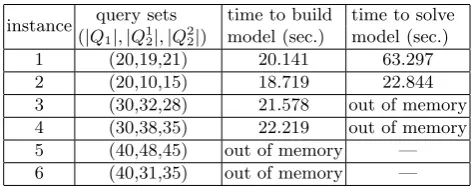
Table 6.Time of solvingIP2 for instances over the 17-attribute TPC-H database
instance query sets (|Q1|,|Q12|,|Q22|)
time to build model (sec.)
time to solve model (sec.)
1 (20,19,21) 20.141 63.297
2 (20,10,15) 18.719 22.844
3 (30,32,28) 21.578 out of memory
4 (30,38,35) 22.219 out of memory
5 (40,48,45) out of memory —
From Table 5, we observe that we could solve all the instances whose number of queries inQ1is no more than 140 based on the 13-attribute database within 10 minutes. However, when we increase the size of the query set, the solver fails to provide an optimal solution within the time limit of 20 minutes. Moreover, from Table 6, CPLEX fails to give an optimal solution for the instances based on the 17-attribute database where the size of the query set grows to 30. The failure is due to memory limitation. In addition, when the size of the query set grows further to 40, we are not able to even build the model due to insufficient memory.
Comparing “the time to build model” with “the time to solve the model” in Tables 2, 4, and 5, we observe that, as the number of queries in each query set of the instance increases, the time required to build the model IP2 grows slowly. At the same time, the time required to solve the model grows relatively fast. For all the instances, the time required to build the model is smaller than the time required to solve the corresponding model IP2. For the instances with larger size of query sets and larger execution times, this difference is quite significant.
4.4 Summary of observations
From the results of the above experiments, we observe that the search spaces for the view sets are significantly reduced in model IP2 compared with model IP1. As a result, the size of the model is much smaller inIP2. This allows us to solve the instances of problem SVS of realistic size using model IP2 to obtain an optimal solution, while IP1 may not able to solve the problem within the time limit. It is also observed that there are some realistic-size instances which could not be solved byIP2.
5
Value of the two-stage stochastic model
In Section 5.1 we compare and contrast the modelSP with a correspond-ing one-stage model, and introduce the value of two-stage versus one-stage. In Section 5.2 we compare the model SP with a two-stage model which is based on the expected value of random events, and introduce the value of stochastic solution. In Section 5.3 we provide several related numerical results.
5.1 Two-stage versus one-stage
In this subsection, we introduce the value of two-stage versus one-stage for solv-ing the SVS problem. In the two-stage stochastic view selection model, we allow for a view replacement at stage 2. Thevalue of two-stage versus one-stage mea-sures the gain obtained via this replacement mechanism. We start by discussing the one-stage model, that is, the model in which we do not allow to drop or replace any materialized views at stage 2. In other words, at time 1 (stage 1), we decide to materialize a set of viewsS under a given space limitb1. We use the views inSto answer all queries inQ1, as well as all queries in the query setQℓ 2 that may occur at time 2 (stage 2), forℓ= 1 toL. We then compare the optimal value of this model with the optimal value of the corresponding two-stage model and define thevalue of two-stage versus one-stage in this context.
Let the decision variablesxi,zijandtℓijbe as defined in Section 2.2. It follows that we could formulate the one-stage problem as an integer programming model that we denote byOS as follows.
(OS) minimize ∑ j∈J1
∑
i∈I1j
dijzij+ L
∑
ℓ=1 pℓ
∑
j∈Jℓ 2
∑
i∈Iℓ 2j
dijtℓij
subject to ∑ i∈I1j
zij = 1 ∀j∈J1
z∑ij≤xi ∀j∈J1, ∀i∈I1j
i∈Iℓ 2j
tℓ
ij = 1 ∀j ∈J2ℓ, ℓ= 1, . . . , L tℓ
ij ≤xi ∀j∈J2ℓ, ∀i∈I2ℓj, ℓ= 1, . . . , L
∑
i∈I1
aixi≤b1
All variables are binary
(51) We note that if we setb2= 0 in modelSP, then the model is equivalent to the model OS.
LetOptv(·) represent the optimal value of a model (·). We have the following observation.
Observation 7 The optimal value ofOSis an upper bound on the optimal value of modelSP, that is,Optv(SP)≤Optv(OS).
uℓi=xi, ∀i∈I2ℓ, ℓ= 1, . . . , L
Then, in model IP1, constraints (33)-(35) are redundant, and constraint (32) becomes
tℓij≤xi ∀j∈J2ℓ, ∀i∈I ℓ
2j, ℓ= 1, . . . , L.
Note that after adding those constraints toIP1, the new IP model is equiv-alent to OS. In other words,IP1 is a relaxation of OS. We thus obtain that Optv(OS) is an upper bound on the optimal value of modelSP, that is,Optv(SP)≤ Optv(OS).
We definethe value of two-stage versus one-stage (V T V O) as the difference between the optimal values of the one-stage and two-stage models, namely,
V T V O=Optv(OS)−Optv(SP). (52) For a given instance of the problem, the corresponding value ofV T V O pro-vides the magnitude of improvement in the optimal response time achieved by allowing the partial replacement of views at stage 2.
5.2 The value of stochastic solution (V SS)
In this subsection, we introduce the value of stochastic solution for the SVS problem. In the literature on stochastic programming [4], thevalue of stochastic solution (V SS) provides the possible gain obtained from solving the stochastic programming model as opposed to solving a model based on expected values. More specifically, for the SVS problem, we consider the model in which we make the first-stage decisions based on the “expected” scenario of stage 2, instead of a number of scenarios with associated probabilities as we do in model SP, and then we make the second-stage decisions given the actual query set occurring at stage 2. We compare this model with the modelSP. The difference between the expected response times is the value of stochastic solution.
In order to examine theV SS from the perspective of the SVS problem, we first consider and define the expected value problem. In this model, instead of having a number of realizations ofQ2, we consider the query workload at stage 2 as a deterministic query setQ2=∪L
ℓ=1Qℓ2, with cost weightpℓfor queryq∈Qℓ2. If a query is in more than one query set from{Qℓ2, ℓ= 1, . . . , L}, the weights are accumulated accordingly. In other words, we can define the weightwj for each queryqj ∈Q2as
wj=
∑
ℓ:qj∈Qℓ2
pℓ (53)
answering the queries occurring at time 1 and the cost of answering the queries occurring at time 2. We now construct a mathematical model for this problem which we refer to asEV.
LetJ2be the set of subscripts for all queries qj ∈Q2. We define V2={vi∈V :vi⊇qfor someq∈Q2}
Note thatV2=∪Lℓ=1V ℓ
2, whereV2ℓ is as defined in Section 2.2. Correspondingly, we define as I2 the set of subscripts associated withV2. For each queryqj∈Q2 we define V2j = {vi ∈ V2 : vi ⊇ qj}. Similarly, we define as I2j the set of subscripts associated withV2j.
We can now define the following second stage decision variables for all views vi ∈V2.
ui=
{
1 if viewvi is materialized at stage 1 and kept at stage 2 0 otherwise
yi =
{
1 if viewvi is materialized at stage 2 0 otherwise
In addition, we define the second stage decision variables tij for all queries qj∈Q2, and for all viewsvi∈V2j.
tij=
{
1 if we use viewvi to answer queryqj at stage 2 0 otherwise
Let the first stage decision variables xi and zij be as defined in Section 2.2. It follows that the expected value problem could be formulated as an integer programming model that we denote byEV, as follows.
(EV) minimize ∑
j∈J1
∑
i∈I1j
dijzij+
∑
j∈J2
∑
i∈I2j
wjdijtij
subject to ∑ i∈I1j
zij = 1 ∀j ∈J1
z∑ij ≤xi ∀j ∈J1, ∀i∈I1j
i∈I1
aixi≤b1
∑
i∈I2j
tij = 1 ∀j ∈J2
tij≤ui+yi ∀j ∈J2, ∀i∈I2j u∑i≤xi ∀i∈I2j
i∈I2
aiyi≤b2
∑
i∈I2
ai(ui+yi)≤b1
All variables are binary
of the stochastic solution measures how poor a decision ( ¯x,z¯) is in terms of the model SP. We define theexpected result of using the EV solution as
EEV = ∑ j∈J1
∑
i∈I1j
dijz¯ij+EQ2Ψ(¯x, Q2) (55)
whereΨ(·) is defined in (20)-(26). We make the following observation.
Observation 8 EEV is an upper bound on the optimal value of modelSP, that is, Optv(SP)≤EEV.
Proof. EEV is equal to the optimal value of model IP1 after fixing the first stage decision variablesxiandzij to be ¯xi and ¯zij, respectively, for alliand all j. Thus,EEV is an upper bound on the optimal value of modelSP.
We compareEEV andOptv(SP), and define thevalue of stochastic solution
(V SS) as the difference between these values, namely,
V SS =EEV −Optv(SP). (56) For a given instance of the problem, the corresponding value ofV SSprovides the magnitude of improvement in the expected response time achieved by solving the stochastic programming model versus solving the smaller expected value problemEV.
5.3 Numerical results
In this subsection we conduct several computational experiments over a number of instances to assess theV T V O and theV SS for the model SP. We observe that the magnitudes of both the V T V O and the V SS vary among instances. This relies on the structure and properties of both the database and the query workloads. We also observe that for each of the two values, there are some instance where the corresponding value is very significant. This indicates that the modelSP is very beneficial over these instances.
Numerical results on V T V O In order to obtain V T V O, the value of two-stage versus one-two-stage, we need to solve the modelOS. Note that the modelOS is equivalent to the deterministic one-stage modelOV IP′ introduced in [2] if we define the frequency fj for each query qj as follows. For each query occurring only at stage 1 we define its frequency as 1, for each query occurring only at stage 2 we define its frequency aswj, and for each query occurring at both stage 1 and stage 2 we define its frequency as 1 +wj, where wj is defined in (53).
fj =
1 ∀j∈Q1−Q2 wj ∀j∈Q2−Q1 1 +wj ∀j∈Q1∩Q2
Thus, we can now apply the exact methods introduced in [2] to solve the model OS.
Example 1 (Continued).For the example introduced in Section 2.1, the optimal value of modelOS is 40.5. As a result, we obtain thatV T V O is 6.5 (=40.5-34). In a computational experiment we constructed and solved a number of in-stances of the two-stage problem with varying sizes over different datasets. For each instance we obtained the corresponding value ofV T V O. We observed that the relative magnitude of V T V O varies among these instances. While in some instances this value is relatively small, in other instances it is quite significant. Following is a numeric example in which the value ofV T V Ois relatively high.
Example 2. We construct this example based on a 13-attribute type I non-symmetric synthetic dataset [8] DI. The master table contains all the possible entries by taking different values over the 13 attributes. The numbers of different values that the 13 attributes take are 2, 2, 2, 2, 3, 3, 3, 3, 4, 4, 4, 4, 4 and 4, re-spectively. We apply a similar approach as in Section 4.1 to obtain the query sets Q1andQ2={Q12, Q22}for this instance. The number of queries in each query set is 20, 15 and 21, respectively. We setp= (0.5,0.5) andb= (b1, b2) = (1632334, 816167). Then the instance is represented by (DI, Q1,Q2,p,b).
We compare the optimal values of modelsSP andOS, and we also report V T V O and the ratio ofV T V O overOptv(SP) in Table 7.
Table 7.Results ofV T V Oover Example 2
Optv(SP) Optv(OS) V T V O V T V O/Optv(SP) 1,810,103 10,892,471 9,082,368 501.760%
We observe that in this instance the value ofV T V Ois more than 5 times the optimal value of modelSP. In other words, in this instance, applying a two-stage model, that is, modelSP, instead of a one-stage model reduces the corresponding response time by more than 80%. Thus, the stochastic view selection model could be very beneficial over some instances.
Numerical results on VSS In order to obtain V SS, the value of stochastic solution, we need to solve the model EV and calculate EEV. In the model EV, we are given a deterministic query set Q2 at stage 2. Thus, the model EV could be considered as a special case of the modelSP where there is only one scenario at stage 2. We can apply a similar approach as in Section 3.2 to reduce the search spaces of views for the model EV, and solve it to obtain the EV solutions. We then plug theEV solutions into equation (55), and solve the second stage problem to obtain EEV.
the first stage solutions over modelsSPandEV. The optimal value of the model SP is 34. We fix the first stage solutions to be as obtained in modelEV, solve model SP, and obtainEEV = 35. Thus,V SS=EEV −Optv(SP) = 1.
Again in a computational experiment, we solved modelEV and calculated the corresponding value EEV over a collection of instances of varying sizes bases on different types of datasets. We then calculated the associated value of V SS and the ratio of V SS over the optimal value ofSP for each instance. We observed that the relative value ofV SS varies among these instances, and that its magnitude depends on both the structure of the underlying database and on the corresponding size of the views, as well as on the structure of the query set. While in some instances the value ofV SS is relatively small, in other instances it can be quite substantial. Following is a specific example in which this value is relatively high.
Example 3. This example is based on a 13-attribute symmetric synthetic dataset [8]DS(13; 2) (denoted asDS for short). Each attribute takes 2 different values, and the master table contains all the possible entries by taking different values over the 13 attributes. The number of queries in query setsQ1,Q2={Q12,Q22} are 20, 19, and 20, respectively. We set b = (17858,8929) and p = (0.5,0.5). Then the instance is represented by (DS,Q1,Q2,p,b).
We compareV SSwith the optimal value of modelSP and report the results in Table 8.
Table 8.Results ofV SSover Example 3
Optv(SP)Optv(EV) EEV V SS V SS/Optv(SP)
27,139 41,841 35,686 8,574 31.49%
As observed in Table 8, it is beneficial to take into account the stochastic properties of the future when performing model formulation of the stochastic view selection problems. In this instance, the expected response time would be more than 31% higher if we used the expected value model EV instead of the stochastic programming modelSP.