Acute Inflammatory Response to Endotoxin Challenge: Model Development, Parameter Estimation, and Treatment Control.

(1)

ABSTRACT

FRANK, DENNIS ONYEKA. Acute Inflammatory Response to Endotoxin Challenge: Model Development, Parameter Estimation, and Treatment Control. (Under the direction of Hien T. Tran.)

Bacterial lipopolysaccharides (LPS; endotoxins) are the major outer surface membrane compo-nents present in almost all Gram-negative bacteria and act as extremely strong stimulators of innate or natural immunity in diverse eukaryotic species ranging from insects to humans. They also induce acute inflammatory response comparable to bacterial infection. Like most biological processes, modeling the inflammatory response involves using highly nonlinear dynamic systems of differential equations with a relatively large number of parameters. Several researchers have within the last seven years developed mathematical models of acute inflammatory response to infection; some of these models are low-order and are biologically irrelevant due to oversim-plification of the real process. The high-order models on the contrary, are highly complex, computationally expensive and constitute challenges in calibrating the model to experimental data.

In the first phase of our work, we propose and validate a number of competing models of acute inflammatory response to compare with a recently developed model in the literature. Our desire to come up with models that can accurately predict the observed dynamics of the pro-and anti-inflammatory cytokines led us to conduct sensitivity analysis, subset selection pro-and parameter estimation in order to obtain accurate parameter values from existing data. Next, we employ a model selection technique to aid with selecting the “best” model among all the potential candidates. In addition, we prove the existence and uniqueness of a solution to our “top choice” model as well as study the model’s steady state and stability behavior.

(2)

c

(3)

Acute Inflammatory Response to Endotoxin Challenge: Model Development, Parameter Estimation, and Treatment Control

by

Dennis Onyeka Frank

A dissertation submitted to the Graduate Faculty of North Carolina State University

in partial fulfillment of the requirements for the Degree of

Doctor of Philosophy

Mathematics

Raleigh, North Carolina 2010

APPROVED BY:

Stephen L. Campbell Negash G. Medhin

John E. Franke Hien T. Tran

(4)

DEDICATION

To my parents, Victor and Beatrice Ureh Frank, who had to sacrifice a lot to provide me with quality education, and to my second mom, Joyce Esuru Osoh, who helped shape my

(5)

BIOGRAPHY

(6)

ACKNOWLEDGEMENTS

Only as I approached the tail end of this chapter of my life did I come to the realization that a Ph.D. is more about the journey than the end result. This entire journey has been one of mixed emotions, personal growth and maturation. In all of these, the most valuable lessons I learned are patience, perseverance and respect for people’s accomplishments. In view of this, I would like to express my heartfelt gratitude to my advisor, Dr. Hien Tran. Thank you for your patience with me. Thank you for being very understanding. Thank you for your guidance and all the time you spent mentoring me.

To my committee members: Dr. Stephen L. Campbell, Dr. Negash G. Medhin and Dr. John E. Franke. Thank you for serving on my committee. I really do appreciate the conversations I had with each of you. Thank you for all your advice and encouraging words. More than anything else, thank you for your wisdom and how in a number of ways your words of wisdom were what made all the difference in my life. Thank you! Thank you!! Thank you!!!

I would also like to take this opportunity to thank the staff of the Mathematics department, es-pecially Denise Seabrooks, Seyma Bennett-Shabbir, Nicole Dahlke, Carolyn Gunton and Char-lene Wallace. I had a lot of personal interactions with all of you, and each of you is simply “awesome.” You always provided “on the spot” help and assistance to me regardless of what you were doing. Thank you very much for your generous hearts.

To my parents, Victor and Beatrice U. Frank as well as Joyce O. Osoh, thank you for inspiring me, and thanks for all your prayers and encouragement. Thank you for believing in me more than I believed in myself, and thanks for giving me the gift of education when I was young. To my siblings, Eze, Odiri, Ike, Chima and Mary Ann, thanks for all your support.

Special thanks to my beloved wife, Ojochide, and the kids, Whanyichukwu, Elemchukwu and Ogochukwu. Thanks for tolerating me for these 5 years. I apologize for those times when I took my academic frustrations out on you guys. Thanks for giving me space and privacy to do my work. Thank you for sharing in my academic joys and sorrows.

(7)

4.3.1 GPOPS . . . 73

4.3.2 SNOPT . . . 75

4.4 Numerical Results . . . 76

4.4.1 Numerical Results for endotoxin challenge level 3mg/kg . . . 77

Chapter 5 Model Predictive Control . . . 84

5.1 Introduction . . . 84

5.2 Historical Background . . . 85

5.3 MPC Methodology . . . 86

5.4 Nonlinear Model Predictive Control (NMPC) . . . 88

5.4.1 Theoretical Issues in NMPC . . . 90

5.4.2 Stability . . . 91

5.4.3 Robustness . . . 93

5.4.4 Output Feedback . . . 95

Chapter 6 NMPC Numerical Results: Reduced 7D Model. . . 97

6.1 Acute Inflammation: NMPC Simulations . . . 99

6.1.1 NMPC Simulations at 3mg/kg endotoxin challenge level . . . 99

6.1.2 NMPCin silico simulations at 6mg/kgand 12mg/kgendotoxin challenge levels . . . 107

6.2 NMPC and UKF . . . 117

6.2.1 Unscented Kalman Filter (UKF) . . . 117

6.2.2 NMPC and UKF at 3mg/kg endotoxin challenge level . . . 118

Chapter 7 Conclusions. . . .122

7.1 Summary . . . 122

7.2 Discussion . . . 124

References. . . .125

Appendices . . . .135

Appendix A 8D Mathematical Model . . . 136

Appendix B 7D Parameters and Plots . . . 140

B.1 Reduced 7D Model Simulation Results . . . 140

(9)

Appendix C Gauss Pseudospectral Method (GPM) . . . 145

Appendix D Sequential Quadratic Programming (SQP) . . . 149

Appendix E 7D Optimal Control Results . . . 152

(10)

LIST OF TABLES

Table 2.1 Parameters of the 8D model . . . 7

Table 3.1 Relative sensitivity ranking for 8D at 3mg/kg endotoxin level, this was calculated using modified L₂ norm . . . 26

Table 3.2 Relative sensitivity ranking for 8D at 12mg/kg endotoxin level, this was calculated using modified L2 norm . . . 28

Table 3.3 8D-15 Model Parameter Estimation . . . 31

Table 3.5 Relative sensitivity ranking for 7D at 3mg/kg endotoxin level, this was calculated using modified L₂ norm . . . 38

Table 3.6 Relative sensitivity ranking for 7D at 12mg/kg endotoxin level, this was calculated using modified L2 norm . . . 40

Table 3.9 Calculated AIC values . . . 52

(11)

LIST OF FIGURES

Figure 2.1 Schematic diagram of the inflammatory response system . . . 8 Figure 3.1 8D relative sensitivity ranking plots at 3mg/kg endotoxin level . . . 25 Figure 3.2 8D relative sensitivity ranking plots at 12mg/kgendotoxin level . . . 27 Figure 3.3 IL6(t) curve fitting plots comparing 8D-15 and 8D at 3mg/kgand 12mg/kg

endotoxin challenge levels . . . 31 Figure 3.4 T N F(t) curve fitting plots comparing 8D-15 and 8D at 3mg/kg and

12mg/kgendotoxin challenge levels . . . 32 Figure 3.5 IL10(t) curve fitting plots comparing 8D-15 and 8D at 3mg/kg and

12mg/kgendotoxin challenge levels . . . 33 Figure 3.6 IL6(t) curve fitting plots comparing 8D-21 and 8D at 3mg/kgand 12mg/kg

12mg/kgendotoxin challenge levels . . . 36 Figure 3.9 7D relative sensitivity ranking plots at 3mg/kg endotoxin level . . . 37 Figure 3.10 7D relative sensitivity ranking plots at 12mg/kgendotoxin level . . . 39 Figure 3.11 IL6(t) curve fitting plots comparing 7D-15 and 8D at 3mg/kgand 12mg/kg

12mg/kgendotoxin challenge levels . . . 45 Figure 3.14 IL6(t) curve fitting plots comparing 7D-21 and 8D at 3mg/kgand 12mg/kg

12mg/kgendotoxin challenge levels . . . 48 Figure 3.17 IL6(t) model validation plots comparing all the models at 6mg/kg

endo-toxin challenge level . . . 49 Figure 3.18 T N F(t) model validation plots comparing all the models at 6mg/kg

en-dotoxin challenge level . . . 50 Figure 3.19 IL10(t) model validation plots comparing all the models at 6mg/kg

en-dotoxin challenge level . . . 51 Figure 4.1 Optimal treatment control at 3mg/kg endotoxin level . . . 77 Figure 4.2 Model solution under optimal treatment control and model solution with

(12)

Figure 4.4 Model solution under optimal treatment control and model solution with

no treatment control at 6mg/kg endotoxin level . . . 81

Figure 4.5 Optimal treatment control at 12mg/kg endotoxin level . . . 82

Figure 4.6 Model solution under optimal control methodology at 12mg/kgendotoxin level . . . 83

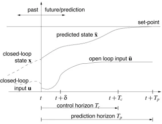
Figure 5.1 Model Predictive Control (MPC) strategy . . . 87

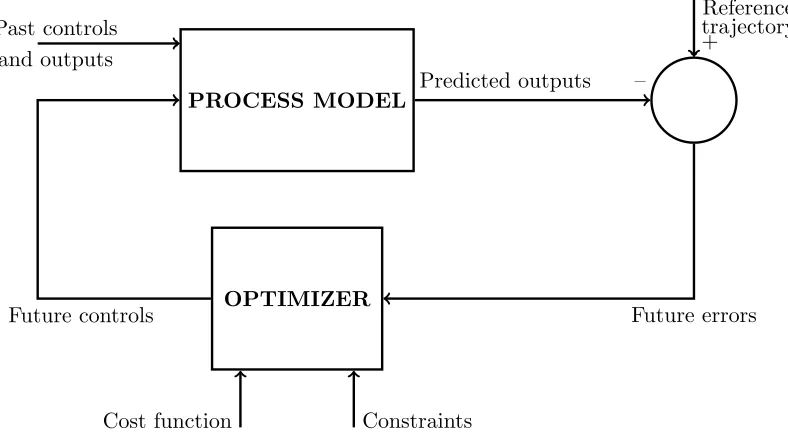
Figure 5.2 Schematic structure of Model Predictive Control (MPC) . . . 88

Figure 5.3 Distribution of MPC applications versus the degree of process nonlinearity [115]. . . 89

Figure 6.1 NMPC simulation ofP(t) at 3mg/kg endotoxin challenge level . . . 100

Figure 6.2 NMPC simulation ofN(t) at 3mg/kg endotoxin challenge level . . . 101

Figure 6.3 NMPC simulation ofD(t) at 3mg/kg endotoxin challenge level . . . 102

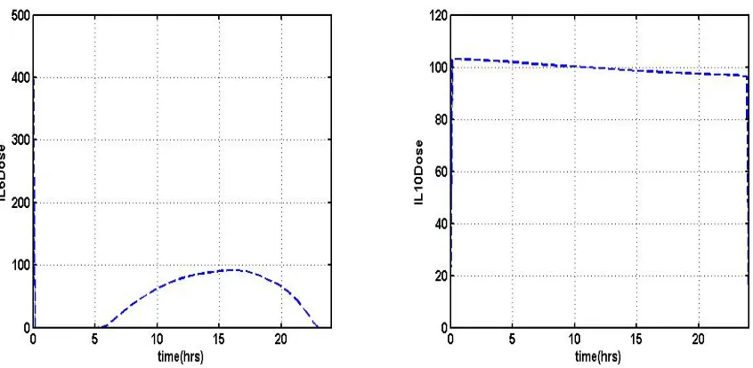
Figure 6.4 NMPC simulation ofIL6(t), andIL6Dose(t) at 3mg/kgendotoxin chal-lenge level . . . 103

Figure 6.5 NMPC simulation ofT N F(t) at 3mg/kg endotoxin challenge level . . . . 104

Figure 6.6 NMPC simulation of IL10(t), and IL10Dose(t) at 3mg/kg endotoxin challenge level . . . 105

Figure 6.7 NMPC simulation ofYIL10(t) at 3mg/kg endotoxin challenge level . . . . 106

Figure 6.10 NMPC simulation ofN(t) at 6mg/kg endotoxin challenge level . . . 109

Figure 6.11 NMPC simulation ofN(t) at 12mg/kgendotoxin challenge level . . . 109

Figure 6.12 NMPC simulation ofD(t) at 6mg/kg endotoxin challenge level . . . 110

Figure 6.13 NMPC simulation ofD(t) at 12mg/kgendotoxin challenge level . . . 110

Figure 6.16 NMPC simulation ofT N F(t) at 6mg/kg endotoxin challenge level . . . . 113

Figure 6.17 NMPC simulation ofT N F(t) at 12mg/kg endotoxin challenge level . . . 113

Figure 6.20 NMPC simulation ofYIL10(t) at 6mg/kg endotoxin challenge level . . . . 116

Figure 6.21 NMPC simulation ofYIL10(t) at 12mg/kgendotoxin challenge level . . . 116

Figure 6.22 NMPC simulation combined with UKF forP(t),N(t), andD(t) at 3mg/kg endotoxin challenge level . . . 119

Figure 6.23 NMPC simulation combined with UKF forIL6(t),IL6Dose(t), andT N F(t) at 3mg/kg endotoxin challenge level . . . 120

(13)

Figure B.1 7D model simulation results at 3mg/kg endotoxin challenge level . . . 141 Figure B.2 7D model simulation results at 6mg/kg endotoxin challenge level . . . 142 Figure B.3 7D model simulation results at 12mg/kg endotoxin challenge level . . . . 143 Figure E.1 Optimal treatment control functions at different endotoxin concentrations 152 Figure E.2 Model solution under optimal treatment control at 3mg/kgendotoxin level.153 Figure E.3 Model solution under optimal treatment control at 6mg/kgendotoxin level.154 Figure E.4 Model solution under optimal treatment control at 12mg/kg endotoxin

(14)

Chapter 1

Introduction

The body responds to bacterial infection or tissue trauma by the activation of acute inflam-matory response. This response, which is non-specific, is considered to be the body’s first line of defense against danger [66]. Inflammation is vital for the removal/reduction of irri-tants to the organism and subsequent restoration of homeostasis. In an attempt to reestablish homeostasis, the inflammatory response is pivotal in clearing invading organisms and offending agents, enhancing wound healing, and promoting tissue repair [140]. This response is made up of a combination of local and systemic mobilization of immune, endocrine, and neurological mediators.

In an ideal situation, the inflammatory response becomes activated, clears the pathogen if there is any infection, begins a repair process and abates. However, inflammation itself can damage otherwise healthy cells which can then further stimulate inflammation. This process can become uncontrollable and lead to tissue damage, organ dysfunction, and ultimately death [24]. To curb the excessive inflammatory response, the body has some regulatory devices such as and anti-inflammatory cytokines that assist with the initiation of tissue repair. The pro-inflammatory cytokines (e.g, interleukin-6 (IL−6)) and tumor necrosis factor-alpha (T N F−α)) up-regulate inflammation and control infections, whereas anti-inflammatory mediators (e.g, interleukin-10 (IL−10)) down-regulate the inflammatory actions, ideally after infection control has been achieved [101].

(15)

sepsis. It is believed that the complex nature of the inflammatory response renders the effect of targeting isolated components of inflammation difficult to predict [76].

Bacterial lipopolysaccharides (LPS), also known as lipoglycans, are highly conserved, highly immunogenic, constituent molecules found in the outer membrane of Gram-negative bacteria, and act as endotoxins. When bacteria are lysed by immune effector cells and molecules, surges of endotoxin may be released into the host, intensifying the inflammatory response and causing further activation of immune effector cells [6]. The administration of antibiotics sometimes results in pulses of endotoxins release from Gram-negative bacteria as the antibiotics attempt to kill the invading bacteria, validating the clinical significance of this subject matter [45]. The fact that direct endotoxin administration in animals and humans is likely to trigger an acute inflammatory response that reproduces many of the features of an actual bacterial infection, such as fever, makes this a compelling reason to develop a valid mathematical model for inves-tigating the inflammatory response [33, 98, 105]. Besides, elevated levels of endotoxin can be lethal.

To this end, the control of inflammatory response to endotoxin challenge has become impera-tive. Thus, we seek to construct a mathematical model that can provide important insights into the global dynamics of the inflammatory process from which therapies may be developed. The advent of the new millennium has brought considerable attention on the development of math-ematical models of acute inflammatory response to infection. This includes the development of both low-order and high-order models of inflammatory response have been developed. For example, in [76] a system of 3 dimensional (3D) ordinary differential equations (ODEs) that consists of a response instigator (pathogen) and early and late pro-inflammatory mediators was proposed. This model was later modified and then extended to incorporate tissue damage as well as anti-inflammatory mediators in [120] to form a 4D model consisting of inflamma-tory stimulus (pathogen), pro-inflammainflamma-tory mediators, tissue damage, and anti-inflammainflamma-tory mediators. To examine repeated endotoxin administration in the context of acute inflamma-tory response, the pathogen equation in [120] was replaced with an endotoxin equation [38]. Although these models provided significant insight into key drivers of inflammatory response outcome, they were not calibrated to any experimental data. On the other end of the spectrum are high-complexity models of the acute inflammatory response cascade [29, 80, 112, 140] . For instance, in [80] the model consisted of 17 ODEs, while [112] had 15 ODEs and [140] contained 31 ODEs. It should be noted that all of these high-order models were calibrated to experimental data.

(16)

was recently developed [126]. This model had a total of 46 parameters. Endotoxin chal-lenges at 3mg/kg, 6mg/kg and 12mg/kg were administered to rats and experimental data for pro-inflammatory cytokines such as interleukin-6 (IL−6) and tumor necrosis factor-alpha (T N F −α) as well as anti-inflammatory cytokine such as interleukin-10 (IL−10) were ob-tained. Data on endotoxin challenges at 3mg/kgand 12mg/kgwere used to calibrate the model, and model validation was performed at endotoxin level of 6mg/kg. In view of the above, this research is motivated in part by:

• The need to come up with a moderate size model that is not as highly complex as that developed in [126], and can be calibrated to the same experimental data on inflammatory cytokines.

• The importance of designing an optimal treatment strategy that can control the effects of acute inflammatory response to endotoxins.

In accordance with our motivation, our contributions at the end of this study to the field of acute inflammatory response are as follows:

1) Development and validation of a reduced mathematical model that can accurately predict acute inflammatory response to endotoxin challenge.

2) Prove the existence and uniqueness of a solution to the reduced mathematical model. 3) Apply a Nonlinear Model Predictive Control (NMPC) scheme in conjunction with the

Un-scented Kalman Filter (UKF) to derive optimal therapeutic interventions for the control of acute inflammation triggered by endotoxins.

To the best of our knowledge, the only work that has been done regarding the control of inflammatory response using NMPC was in [39] (as at the time of writing this thesis, this paper though has been submitted for publication, is yet to be published). Besides, the work ([39]) used a low-order simulated model that was not calibrated to any experimental data.

This work is organized in two main parts. Part I which comprises Chapters 2 and 3 deals with thederivation of mathematical models of acute inflammatory response to endotoxin challenge. In Part II, we focus our attention on the derivation of optimal treatment controls to modulate acute inflammation; this part contains Chapters 4 through 6. For the remaining of this chapter, we will briefly describe the contents of the chapters in this thesis.

(17)

We then present the reduced model equations describing the acute inflammatory response sys-tem to endotoxin challenge. We also presented a brief introductory background on Sensitivity analysis, Subset selection and Parameter estimation since they are the mathematical tools used to construct and calibrate our models with existing data. We conclude this chapter with a description of a model selection criterion called Akaike Information Criterion (AIC) [3]. We began Chapter 3 by displaying the relative sensitivity rankings at 3mg/kg and 12mg/kg endotoxin challenge levels for both 8D and the reduced model, respectively. With the aid of subset selection, the most linearly independent sensitive parameters are identified for all the models we proposed; this information is useful in the calibration of these models to the observed data on cytokines. Next, we present the model comparison and validation plots as well as AIC results. Following the construction of the reduced model in the previous chapter, we show a rigorous mathematical analysis of the existence and uniqueness proof for a solution of the reduced model as well as conduct steady state and stability analysis.

Optimal control methodolody is introduced in Chapter 4 to study our model under open-loop optimal control based treatment strategies. Two control inputs representing treatment therapies are added to the model and an open source solver known as GPOPS is used to solve the optimal control problem numerically. Lastly, we summarize thein silicosimulation results of the optimal control solutions for each of the three endotoxin challenge levels (3mg/kg,6mg/kg and 12mg/kg).

(18)

Part I

(19)

Chapter 2

Model Derivation

This chapter deals with the materials and methods for the derivation of a mathematical model of acute inflammatory response to endotoxin challenge. To this end, we discuss the formation of “modified 8D”1 models from carrying out sensitivity and parameter identification analyses on the original 8D model. In addition, we elucidate our decision to construct a reduced model. We will wrap the chapter up by introducing a quantitative model selection technique use for model comparison. For completeness, we will begin with a summary of the 8D model developed in [126]. The interested reader should consult this reference for a comprehensive description of the 8D model development.

2.1

8D Model Overview

Experimental data on cytokines at 3mg/kg and 12mg/kg endotoxin challenge levels were used to calibrate the 8D model. The original experiments were conducted on three cohorts of Sprague-Dawley rats weighing approximately 200gand were performed according to an IACUC-approved protocol at the University of Pittsburgh, Department of Surgery, to study the acute inflammatory response to endotoxin insults at various concentration levels. The rats received endotoxin (Escherichia Coli) at levels of either 3mg/kg, 6mg/kg, or 12mg/kg, intraperitoneally. Blood samples were collected at time points 0, 1, 2, 4, 8, 12 and 24 hours after endotoxin administration. Concentrations of pro- and anti-inflammatory cytokines such as interleukin-6 (IL6), interleukin-10 (IL10) and tumor necrosis factor-α (T N F) were measured in triplicate using commercially available ELISA kits (R & D Systems, Minneapolis, MN).

1

(20)

Table 2.1: Parameters of the 8D model

No. Parameter Value Unit No. Parameter Value Unit

1† dP 3 hr−1 24 xIL6IL10 1.1818 _mLpg

2 kN 5.5786e7 hr−1 25 kIL6IL6 122.92 −

3 xN 14.177 N −unit 26 xIL6IL6 1.987e5 _mLpg

4 dN 0.1599 hr−1 27‡ xIL6CA 4.2352 _mLpg

5 kN P 41.267 N−unit_mg ·kg 28 kT N F 3.9e-8 _mL_·_N₋pg_unit1.5

6 kN D 0.013259 N_D−−unitunit 29 dT N F 2.035 hr

−1

7 xN T N F 1693.9509 _mLpg 30 xT N F IL10 2.2198e7 _mLpg

8 xN IL6 58080.742 _mLpg 31‡ xT N F CA 0.19342 _mLpg

9‡ xN CA 0.07212 _mLpg 32 kT N F T N F 1.0e-10 −

10 xN IL10 147.68 _mLpg 33 xT N F T N F 9.2969e6 _mLpg 11 kN T N F 12.94907 − 34 xT N F IL6 55610 _mLpg

12 kN IL6 2.71246 − 35 kIL10T N F 2.9951e-5 −

13 kD 2.5247 D−_hrunit 36 xIL10T N F 1.1964e6 _mLpg

14 dD 0.37871 hr−1 37 kIL10IL6 4.1829 −

15 xD 1.8996e7 N −unit 38 xIL10IL6 26851 _mLpg

16‡ kCA 0.154625e-8 _mL_·_hrpg_·_N₋_unit 39 kIL10 1.3374e5 _mLpg_·_hr

17‡ dCA 0.31777e-1 hr−1 40 dIL10 98.932 hr−1

18‡ † sCA 0.004 _mLpg_·_hr 41 xIL10 8.0506e7 N −unit

19 kIL6T N F 4.4651 − 42† sIL10 1187.2 _mLpg_·_hr

20 xIL6T N F 1211.3 _mLpg 43 xIL10d 791.27 _mLpg 21 kIL6 9.0425e7 _mLpg_·_hr 44 kIL102 1.3964e7 YIL10_hr−U nit

22 dIL6 0.43605 hr−1 45 dIL102 0.0224 hr−1

23 xIL6 1.7856e8 N −unit 46 xIL102 37.454 D−unit

‡

Parameter not part of reduced model

†

Parameter not estimated in both reduced and 8D models

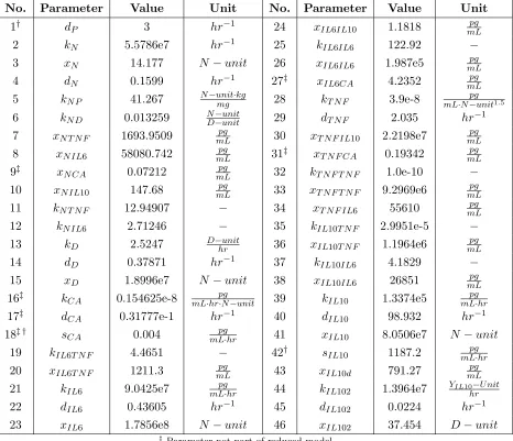
The 8D model comprised of eight ordinary differential equations with the following states: En-dotoxin concentration (P(t)); total number of activated phagocytic cells (N(t)), which includes all activated immune response cells, such as neutrophils, monocytes, etc.; a non-accessible tissue damage marker (D(t)); concentrations of pro-inflammatory cytokines interleukin-6 (IL6(t)) and tumor necrosis factor-α(T N F(t)); concentration of the anti-inflammatory cytokine interleukin-10 (IL10(t)); a tissue damage driven non-accessible IL-10 promoter (YIL10(t)); and a

(21)

of 46 parameters of which 43 were estimated. These parameters and their nominal values are displayed in Table 2.1. The actual representation of the 8D ODE system described in [126] is given in Appendix A.

P

N D

YIL10 IL−10

CA

TNF−α IL−6

Up-regulate (

→

) Down-regulate (

99K

)

Figure 2.1: Schematic diagram of the inflammatory response system challenged by endotoxin [36, 126]

(22)

andCA(t)) [53]. The pro-inflammatory cytokines exert positive feedback on the system; hence, further activateN(t) and up-regulate other cytokines [14, 53]. The anti-inflammatory mediators exert negative feedback on the system; hence,IL10(t) andCA(t) inhibit the activation ofN(t) and down-regulate other cytokines [107, 110]. The model also incorporates tissue damage due to activated phagocytic cells, represented by a damage marker,D(t). Tissue damage further up-regulates activation ofN(t) [93] and also contributes to up-regulation ofIL10(t) [55, 72].

2.2

Derivation of Model

In this section, the various mathematical tools used in creating “modified 8D” and the reduced models are discussed. First, we justify our rational for building adequate reduced models capable of predicting the observed dynamics of pro- and anti-inflammatory cytokines.

2.2.1 Derivation of Reduced Model

In order to derive a reduced model, we used information in [38, 39, 120, 126] to categorize the state variables in the 8D model into five groups:

• Endotoxin concentration: P(t)

• Inflammation : Total number of activated phagocytic cells (N(t))

• Collection of pro-inflammatory cytokines: IL6(t) andT N F(t)

• Collection of anti-inflammatory mediators: IL10(t) andCA(t)

• Tissue damage: D(t) andYIL10(t).

(23)

As part of our model building cycle, we intend to calibrate our models to the experimental data on inflammatory cytokine. Since we do not have access to the original experimental observations, Engauge digitizer version 4.1 [46] was used to digitize the data in [126]. Plots of the digitized data were compared visually with the reported data. Engauge digitizer is an open source digitizing software that converts an image file of a graph or map into numerics [46]. Finally, we will adopt the same approach used in the 8D model building cycle by calibrating the 7D and “modified 8D” models at endotoxin levels 3mg/kg and 12mg/kg, respectively. Endotoxin challenge level 6mg/kg will then be used for model prediction.

2.2.2 7D ODE Model

The reduced 7D mathematical model of acute inflammatory response to endotoxin challenge is described in this section, the model consist of 7 ordinary differential equations and 40 parame-ters.

dP(t)

dt =−dp·P(t) (2.1)

dN(t)

dt =kN·

Γ(t) xN+Γ(t)

−dN ·N(t) (2.2)

dD(t)

dt =kD·

N(t)6

x6_D+N(t)6 −dD·D(t) (2.3)

dIL6(t)

dt =kIL6·

N(t)4 x4

IL6+N(t)4

·Ω(t)−dIL6·IL6(t) (2.4)

dT N F(t)

dt =kT N F·N(t)

1.5_Φ(t)₋_d

T N F ·T N F(t) (2.5) dIL10(t)

dt =kIL10·

N(t)3

x3

IL10+N(t)3

·Ψ(t)−Θ(t) +YIL10(t) +sIL10 (2.6)

dYIL10(t)

dt =kIL102·

D(t)4 x4

IL102+D(t)4

−dIL102·YIL10(t), (2.7)

with the initial condition

P(0) = 3, 6, or12; N(0) = 0; D(0) = 0; IL6(0) = 0 T N F(0) = 0; IL10(0) = sIL10·xIL10d

dIL10·xIL10d−sIL10

(24)

In addition, from Equation (2.2)

Γ(t) = [kN P ·P(t) +kN D·D(t)]·f DNN IL10(t)·γ(t)

γ(t) = (1 +kN T N F ·f U PN T N F(t))·(1 +kN IL6·f U PN IL6(t))

f DNN IL10(t) =

xN IL10

xN IL10+IL10(t)

(2.9)

f U PN T N F(t) =

T N F(t) xN T N F +T N F(t) f U PN IL6(t) =

IL6(t) xN IL6+IL6(t)

,

from Equation (2.4)

Ω(t) = (1 +kIL6T N F ·f U PIL6T N F(t) +kIL6IL6·f U PIL6IL6(t))·f DNIL6IL10(t)

f DNIL6IL10(t) =

xIL6IL10

xIL6IL10+IL10(t)

f U PIL6T N F(t) =

T N F(t) xIL6T N F +T N F(t)

(2.10)

f U PIL6IL6(t) =

IL6(t) xIL6IL6+IL6(t)

,

from Equation (2.5)

Φ(t) = [1 +kT N F T N F ·f U PT N F T N F(t)]·f DNT N F IL10(t)·f DNT N F IL6(t)

f DNT N F IL10(t) =

xT N F IL10

xT N F IL10+IL10(t)

f DNT N F IL6(t) =

xT N F IL6

xT N F IL6+IL6(t)

(2.11)

f U PT N F T N F(t) =

T N F(t) xT N F T N F +T N F(t)

,

(25)

Ψ(t) = 1 +kIL10IL6·f U PIL10IL6(t) +kIL10T N F ·f U PIL10T N F Θ(t) =dIL10·f DNIL10d(t)·IL10(t)

f DNIL10d(t) =

xIL10d xIL10d+IL10(t)

(2.12)

f U PIL10IL6(t) =

IL6(t)4 x4_IL₁₀_IL₆+IL6(t)4

f U PIL10T N F =

T N F(t) xIL10T N F +T N F(t)

.

We will mimic the description of the original 8D model [126] in describing the 7D model. The dynamics ofP(t) are described in Equation (2.1); P(t) decays exponentially with a decay rate of dP. We used the same value for the decay rate as in [126], which is fixed at 3hr−1. This value is also in accordance with published results [38, 79, 142].

Equations (2.2) and (2.9) denote the total number of activated phagocytic cellsN(t). Resting phagocytic cells are activated by the presence of endotoxin,kN is the rate of activation ofN(t) anddN is the elimination rate. N(t) is activated byP(t) andD(t) viaΓ(t) as described in Equa-tion (2.9). FuncEqua-tions with nomenclaturef U Pij(t) and f DNij(t) represent up-regulating (UP) and down-regulating (DN) effects of inflammatory cytokinejon cytokinei. These functions are bounded between 0 and 1 and are dimensionless. The up-regulating functions, f U PN T N F(t) andf U PN IL6(t),in Equation (2.9) are Michaelis-Menten type equations; as the concentrations

increase, the values of these functions approach 1 asymptotically. Gain parameters kN T N F and kN IL6 scale the up-regulating functions to get the real effect of N(t). The inhibitory

ef-fects of IL10(t) are represented by the down-regulating function f DNN IL10; as the level of

IL10(t) raises, f DNN IL10 approaches 0 asymptotically. xN, xN T N F, xN IL6 and xN IL10 are

the half-saturation parameters that determine the concentration levels of the states so that the corresponding f U PN T N F(t), f U PN IL6(t), and f DNN IL10 functions will attain half of its

saturation point.

Equation (2.3) corresponds to the tissue damage instigated by the inflammatory response to endotoxin challenge. kD is the rate of production of D(t), dD is the corresponding rate of elimination, andxD is the half-saturation parameter. Increased levels ofD(t) further activates N(t) and thus produced IL10(t). A 6th order Hill function was used to accurately capture the data [126].

(26)

behav-ior is captured by the up-regulating functions, f U PIL6T N F(t) and f U PIL6IL6(t), respectively,

in Equation (2.10); the down-regulating function, f DNIL6IL10(t), is the inhibitory effect and

dIL6is the clearance rate ofIL6(t). A 4thorder Hill function was used to accurately capture the

data [126], andxIL6, xIL6T N F, xIL6IL6 and xIL6IL10 are the half-saturation parameters.

The pro-inflammatory cytokineT N F(t) is described in Equations (2.5) and (2.11), respectively. T N F(t) is produced by the activation of N(t); kT N F is the rate production of T N F(t) and dT N F is the clearance rate. An exponent of 1.5 was assigned to N(t) to accurately represent the rapid production and elimination ofT N F(t); the justification for this choice is discussed in [126]. The f U PT N F T N F(t) function in Equation (2.11) is the up-regulating effect of T N F(t) on its own production; whereasf DNT N F IL10(t) andf DNT N F IL6(t) are the inhibitory effects.

xT N F T N F, xT N F IL10 and xT N F IL6 are the half-saturation parameters.

The concentration of the anti-inflammatory cytokineIL10(t) is represented in Equations (2.6) and (2.12), respectively. IL10(t) is up-regulated by the f U PIL10IL6(t) and f U PIL10T N F, re-spectively. This is described in Equation (2.12); the production ofIL10(t) in the basal state is given by sIL10, which can be obtained from the experimental data. It was shown in [125] that

the rate of elimination of IL10(t) is inversely proportional to the circulating concentration of IL10(t), this is depicted by the down-regulating functionf DNIL10d(t) in Equation (2.12) along-side the parameterdIL10. xIL10, xIL102, xIL10IL6, xIL10T N F and xIL10dare the half-saturation parameters.

The dynamics of YIL10(t) are described by Equation (2.7). kIL102 is the rate of production of

YIL10(t) and dIL102 is the rate of elimination. A 4th order Hill function, which is driven by

D(t), is used to model YIL10(t),

2.2.3 Sensitivity Analysis

(27)

To formally introduce this concept, we consider a nonlinear system of the form: dy(t)

dt =f(t,y;q), y∈R

n_, _q_∈

Rm (2.13)

z(t) =h(t,y,q), z∈Rr, (2.14)

with the initial condition

y(0) =y0, (2.15)

wherey, zandqdenote state, output and parameter vectors, respectively. We are interested in howzchanges with respect toq(sensitivity), i.e., ∂_∂z(_qt). To determine the sensitivity of the out-putszwith respect to the parametersq,we take the partial derivative of Equation (2.14)

∂z ∂q =

∂h ∂y

∂y ∂q+

∂h

∂q. (2.16)

In order to obtain ∂_∂y_q we need to derive a system of differential equations for the sensitivities by differentiating both sides of (2.13) with respect to qand switching the order of differentiation to yield the sensitivity equations

d dt

∂y ∂q =

∂f ∂y

∂y ∂q+

∂f

∂q. (2.17)

We assume that the initial conditions of the sensitivities are zero (that is, ∂y(0)_∂_q = 0) since the initial conditions of the model would not be considered to be dependent on the model parameters. By coupling equations (2.13) and (2.17), we have ann+nm dimensional system of differential equations for both the model and the sensitivities. Coupling ensures that the solution fory(t) is sufficiently accurate to solve the sensitivity system to the desired accuracy. On the other hand, if the equations are not coupled, some interpolating scheme will be required when the differential equations are solved numerically using adaptive mesh methodologies. The partial derivatives ∂zi(t)

∂qj , fori= 1. . . r, j= 1. . . m,are known as first-order sensitivities [30,

64]. The second-order sensitivities, ∂2zi(t)

∂qj∂qk, fori = 1. . . r, j, k = 1. . . m can also be calculated

and they ascertain the sensitivity of the the first-order sensitivity ∂zi(t)

∂qj with respect to changes

(28)

In this work, we only consider the first-order sensitivity of the experimental data (IL6(t), T N F(t) andIL10(t)). In addition, our output equations (Equation (2.14)) are linear functions of the state

z(t) =Cy(t), (2.18)

whereCis given by

C= 

 

0 0 0 1 0 0 0 0 0 0 0 1 0 0 0 0 0 0 0 1 0





. (2.19)

From the experiment carried out in [126], three parameters were specified in the 8D model; the clearance rate of endotoxin concentrationP(t) captured by dp was obtained from the literature [79, 142], while sCA and sIL10 were extracted from the experimental data. This implies that

in the construction of “modified 8D” z ∈ _R3

+ and q ∈ R43+; where Rr+ is the space of

r-tuple nonnegative real numbers, z ∈ _R3

+ denote the 3 outputs (measured cytokines) and q ∈

R43+ indicate the 43 parameters we wish to investigate their sensitivity levels for each output.

Similarly, in building the reduced 7D model,z ∈_R3

+ andq∈R38+ because we excluded dp and sIL10 in the 7D model sensitivity analysis; sCA is not in the reduced model since it is linked withCA(t) which was removed to form 7D.

The matrix S(t) = ∂zi(t)

∂qj for i = 1. . .3, j = 1. . . m is known as the sensitivity matrix (or

the Jacobian matrix or the Fr´echet derivative [64]) at time t, where m = 43 for 8D and m = 38 for 7D depending on the model we wish to analyze. S(t) can be normalized by RS(t) = ∂zi(t)

∂qj

qj

zi(t), which is known in the literature as relative sensitivity matrix at time t

(here t = 1,2,4,8,12 and 24. These represent the time points blood samples were taken in the experiment). Let RS¯ be the relative sensitivity matrix across all time period; this matrix can be constructed by stacking the time dependent relative sensitivity matrices RS(t) fort= 1,2,4,8,12 and 24 as follows

¯ RS=           

RS(t= 1) RS(t= 2) RS(t= 4) RS(t= 8) RS(t= 12) RS(t= 24)

          

18×m

(29)

Note that ¯RSwill be constructed for endotoxin dose levels 3mg/kgand 12mg/kg,respectively. Sensitivity computations were carried out using a relative and generalized sensitivity analysis solver called “tssolve” [11]. This “tssolve” solver uses Automatic Differentiation (AD) [49] to compute the partial derivatives in Equations (2.16) and (2.17), respectively. The computa-tions were performed using MATLAB version “R2009a” ( c2009 The Mathworks Inc., Natick, MA).

Finite difference methods can also be utilized in the approximation of the partial derivatives contained in the sensitivity equations (Equations (2.16) and (2.17)). For example, [1, 36, 64, 108] used finite differences in their respective computations, while [37, 50] made use of AD and [44] employed both methods. Whenever numerical approximation methods such as finite difference is utilized, it is always important to consider the relationship between the difference increment used in the computation of the derivative and the accuracy of the solution obtained from the integrator. However, AD does not have such considerations since it is a “machine precision exact” method that breaks down a function into small component operations before taking derivatives by applying chain rule.

The relative sensitivity matrix computed in Equation (2.20) yields sensitivity information as a function of time. In any case, our priority in this work is to distinguish those model dynamic parameters that significantly influence the outputs of our process over time. To achieve this goal, we compute the relative sensitivity ranking using a modified L2 norm,

∂zi ∂qj 2 · qj max zi

=

" 1 tf −t0

Z tf

t0 ∂zi ∂qj 2 dt #1 2 · qj max zi

. (2.21)

In general, therelative sensitivity ranking contain information regarding the number of param-eters that are most sensitive to each output since it ranks the model paramparam-eters according to their respective sensitive levels. Finally, it is noted that there are other norms adapted in the literature to compute the sensitivity value. For example,

in [1], anL2 norm of the form was used

v u u t 1 Nj Nj X i=1 ∂z ∂qk

(tij_;_qj₎_q k 2 ,

whereas anotherL₂ norm of the form was used in [37]

kf(t)k2₂= Z

(30)

and [44] employed an unspecified norm of the form

kSjk(t, q0)k=

dyj(ti, q0)

dqk

qk yj(ti, q0)

.

2.2.4 Subset Selection

We will begin this section by introducing the concept ofidentifiability with two simple illustra-tions.

Problem 2.2.1 This problem is taken from [32], which was first discussed in [16]. Consider the first-order model:

dx(t)

dt =−p1x(t) +p2u(t), x(0) = 0 (2.22)

y(t) =p3x(t). (2.23)

In this problem,x(t) represents the concentration of a drug introduced into a biological system, u(t) is a test-input injection of the drug of known wave form and in mass units, and y(t) is a temporal measurement of the drug concentration in the system, say by bioassay. There are three parameters in the model: p1,the fractional rate constant for the drug; p2 is the inverse of

its distribution volume and p3, the unknown proportionality constant for the bioassay measure

of drug concentration. For any known u, the explicit solution of Equations (2.22)and (2.23)is given by

y(t) =p2p3

Z t

0

e−p1(t−τ)_u₍_τ₎_dτ. _(2.24)

If the drug is introduced rapidly as a brief pulse of unit magnitude, i.e., an approximation impulse u(t) =δ(t), one obtains the more familiar solution

y(t) =p2p3e−p1t. (2.25)

Semi-logarithmic plot of the data represented as y(t) for this model yields the coefficient A ≡

p2p3 and exponent λ≡ p1. Thus only p1 and the product p2p3 can be determined and not p2

or p3. When this happens, the model is said to beunidentifiable. If p2 or p3 were known, or

related in a known way, all parameters could be uniquely determined from y(t). In this case, we say the model (or model parameters) is (are) uniquely identifiable.

(31)

Consider an m by P output sensitivity function matrix with respect to the parameters, S(t,p) ≡ [∂y_∂p(t,p)

j ], evaluated at a nominal p

0_{. To define this inherently local concept, let} ₄_p

denote a local perturbation about a nominal p0_{, i.e.,} ₄_p _≡_p₋_p0_, _{which gives rise to a local}

perturbation 4y in the output, i.e.,4y≡y(t,p)−y(t,p0).Then

4y∼=S4p. (2.26)

A structure is sensitivity identifiability if (2.26) can be solved uniquely (in the local sense) for4p.This is the case if and only if the column rank of the matrixS is equal toP, the number of unknown parameters, or

det(STS)6= 0. (2.27)

One of the drawbacks of sensitivity analysis is that it identifies “sensitive” parameters that are both unidentifiable (linearly dependent) as well as identifiable (linearly independent). In such situation, subset selection can be employed to separate the most linearly independent sensitive parameter from the rest. These become the identifiable parameters and the less identifiable set will be fixed to some nominal values during the optimization process. Subset selection methodologies for partitioning the parameter space into well-conditioned and ill-conditioned subsets were described in [50]. Similarly, the following subset selection methods were discussed in [108];

i. QR Factorization with column pivoting ii. SVD followed by QR with column pivoting iii. Gu-Eisenstat’s strong rank revealing QR iv. SVD followed by Gu-Eisenstat’s SRRQR.

(32)

on the relative sensitivity matrix RS¯ in (2.20) to obtain the most identifiable parameters at endotoxin levels 3mg/kg and 12mg/kg, respectively. In addition, we favored this algorithm because it is relatively easy to implement.

The SVD followed by QR with column pivoting algorithm is outlined below.

• Compute the SVD of ¯RS=UΣVT and determine the numerical rank ˆr of ¯RS. Hence, we employed the technique described in [50] to determine ˆr as follows

ˆ

r= max i

|σi|

|σ1|

> kRS¯ km

,

where σi represent the sorted singular values of RS¯ such that σ1 = max{σi}, m is the number of parameters, which corresponds with the number of columns in RS¯ and the toleranceis a problem dependent constant. Usuallyis the machine precision tolerance; for this work =3.55e-15. The MATLAB code for computing the numerical rank is as follows:

Code: [row col]=size(RS); sigma=svd(RS);

ratio=abs(sigma)/abs(sigma(1));

NumRank=find(ratio> eps(norm(RS))*norm(RS)*col,1,‘last’);

• LetV = [Vrˆ VN−rˆ] whereVrˆis the first ˆr columns ofV.

• Perform a QR factorization with pivoting on V_r_ˆT to obtain V_r_ˆTP =QR.

QR with column pivoting will align the linearly independent columns of ¯RS to the left and the permutation matrixP contains the information on how the columns of ¯RSwere repositioned.

• Choose as the subset of components of x the first ˆr components of PTx, where x = [1,2,3, . . . ,43]T for 8D andx= [1,2,3, . . . ,38]T for 7D.

An extension of theSVD followed by QR with column pivoting algorithm that applies its eigen-value decomposition on the Hessian matrix was proposed in [138]. This algorithm is claimed to be more appropriate for nonlinear least squares estimation; the interested reader is referred to [64] for an application of this method.

(33)

values ˆσi. RS¯ has a numerical rank ˆr if the ˆσi satisfy

ˆ

σ1 ≥ . . . ≥σˆˆr> δ≥σˆˆr+1≥ . . . ≥σˆn.

Usually, the tolerance δ is chosen to be consistent with the machine precision, for example, δ = ukRS¯ k∞. If the relative error in the data is larger than u, then δ should be bigger, for

instance, if the entries in ¯RS are correct to two digits thenδ = 10−2kRS¯ k∞.[44] applied this

approach with the 2-norm rather than the∞-norm. Lastly, subset selection can also be applied on the generalized sensitivity matrix ¯S, which can be constructed by stacking the time dependent matricesS(t=i) for eachitime point, or the Fisher Information Matrix (FIM), ¯STQ−1S¯where Q is the measurement covariance matrix. The choice of matrix to use is dependent on how well-conditioned /ill-conditioned the problem is; we used the relative sensitivity matrix RS¯ because of the large variation in the order of magnitude of the experimental data.

2.2.5 Parameter Estimation

The goal of parameter estimation (also known as inverse problem or model calibration) is to obtain parameter values of a model that give the best fit to a set of experimental data. To carry out parameter estimation the free parameters must be assigned nominal values that serve as an “initial guess” before commencing the optimization process [85]. The most convenient approach to estimate unknown parameters is from available data; this is usually achieved by calibrating the model to reproduce the experimental results in the best possible way. This calibration is carried out by minimizing a given cost function that measures the goodness of fit [124]. The cost functions, which are represented by bayesian estimator, maximum likelihood estimator, and (weighted) least squares estimator, have been shown to perform relatively well in practice. The bayesian estimation, which happens to be the most complicated, requires the parameter probability distribution and the conditional probability distribution of the measurements for the specified parameters to be parameterized. The least squares estimation, considered to be the least complicated, can be carried out effectively with the availability of observed data, or in silico simulated data [87, 124].

The following potential pitfalls and difficulties when conducting parameter estimation for dy-namic systems were outlined in [130]:

• Lack of convergence to local solutions. This arises when only bad starting values for the parameters are used.

(34)

• The cost function appears very flat in the neighborhood of the solution.

• Some of the terms in the system’s dynamics are non-differentiable.

In addition, Schittkowski [130] classified the existing methods for parameter estimation for dynamic systems into two main groups (the excerpt is from [124]):

1) Initial value methods (also known as single shooting): The parameter estimation problem is solved as a nonlinear optimization (NLO) problem which requires the solution of an inner initial values problem (IVP) for each function evaluation. The outer NLO is usually solved using Levenberg-Marquardt or Gauss-Newton methods. These methods are very efficient and converge globally to the correct solution when a good initial guess for the parameters is specified, otherwise, they converge to local solutions. As these NLOs are frequently multimodal, a lack of fit could be due to convergence to one of such local solutions, even if the model can represent the data perfectly well.

2) Multiple shooting ([21, 136]): Here the dynamic state variables are discretized in some way, leading to larger NLOs (i.e., more degrees of freedom) but avoiding the need of solving an inner IVP. Also, it has been shown that this method does not introduce as much multi-modality as single shooting methods. However, since the resulting large NLO is usually solved using Gauss-Newton methods, which are of local nature, it can still converge to a local solution, especially when only a poor initial guess is available.

(35)

JIL63(q) =

1 maxj(yIL63

j(j=1,...,7)) 7

X

i=1

[yIL63

i −y(ti,q)IL63]2, IL6(t)at3mg/kg, (2.28)

JTNF3(q) =

1

maxj(yT N F_j₍_j₌₁3_,...,₇₎)

7

X

i=1

[yT N F3

i −y(ti,q)

T N F3_]2_, _{T N F}₍_t₎_at₃_mg/kg, _(2.29)

JIL103(q) =

1 maxj(yIL103

j(j=1,...,7)) 7

X

i=1

[yIL103

JIL612(q) =

1

maxj(yIL_j₍_j6₌₁12_,...,₇₎)

7

X

i=1

[yIL612

JTNF12(q) =

1

maxj(yT N F_j₍_j₌₁12_,...,₇₎)

7

X

i=1

[yT N F12

i −y(ti,q)

T N F12_]2_{, T N F}₍_t₎_at₁₂_mg/kg, _(2.32)

JIL1012(q) =

1 maxj(yIL1012

j(j=1,...,7)) 7

X

i=1

[yIL1012

where yk

i is the experimental data at time t = i for state variable k, y(ti,q)k is the model prediction at timeti forqmodel parameters and state variablekand maxj(yjk) is the maximum value of the experimental data over all time points for state variable k.

Combine (2.28) to (2.33) to form the desired cost function that we aim to minimize:

K(q) =JIL63(q) +JTNF3(q) +JIL103(q) +JIL612(q) +JTNF12(q) +JIL1012(q), (2.34)

(36)

2.3

Akaike Information Criterion (AIC)

AIC [3] is amodel selection tool commonly used to compare different models quantitatively. It was developed by a Japanese statistician called Hirotsugu Akaike in 1971 to measure a model’s goodness of fit. AIC measures the amount of information lost when a given model is used to describe the behavior of a real system. When two or more models having different number of parameters are compared, the model with the lowest AIC value is preferred. The formula for calculating AIC is given by

AIC =kln

J k

+ 2p, (2.35)

J= 1 maxj(yj)

n X

i=1

[yi−y(ti,q)]2, (2.36)

where k is the total number of data points,p is the total number of model parameters,J is a nonlinear least-squares method with a normalized residual, y(ti,q) is the model prediction at time ti for q parameters, yi is the experimental data, and maxj(yj) is the maximum value of the experimental data over all time points.

(37)

Chapter 3

Model Analysis

3.1

8D Relative Sensitivity Ranking

We examine the relative sensitivity ranking results of the parameters forIL6, T N F and IL10 at 3mg/kg and 12mg/kg endotoxin challenge levels, respectively. These results are obtained from the 8D model with the primary goal of identifying the most sensitive parameters that will be used to construct “modified 8D” models.

3.1.1 8D Relative Sensitivity Ranking at 3 mg/kg endotoxin challenge level

Figure 3.1 shows the relative sensitivity ranking plots of the parameters for each inflammatory cytokine.

(38)

disad-vantage with this approach is that it is very cumbersome to implement. We implemented the second technique in this work with a 20% perturbation for the case of the reduced 7D relative sensitivity ranking plots in Figures 3.9 and 3.10.

Figure 3.1: 8D relative sensitivity ranking plots at 3mg/kg endotoxin level for IL6, T N F and IL10

Table 3.1 contains essentially the same information with Figure 3.1. However, this table identi-fies each parameter, the corresponding rank, and the computed modified L₂ norm value using Equation (2.21). It is easy to observe from the table that the ranks of some parameters vary widely across the different inflammatory cytokines, for instance, kD is ranked 15th for IL6, 29th for T N F and 1st for IL10. Other parameters with similar characterization are dD, xD and dIL6. Meanwhile, there was no variability in the ranks of the least sensitive parameters:

(39)

Table 3.1: 8D relative sensitivity ranking at 3mg/kg. Number in parenthesis is the computed

L2 norm; the prior number is the rank: 1 implies most sensitive and 43 is least sensitive. Parameter IL6Rank T N F Rank IL10Rank

kN 4 (0.7985) 5 (0.2360) 4 (2.7549)

xN 10 (0.3435) 7 (0.0915) 7 (1.2260)

dN 16 (0.2455) 14 (0.0326) 6 (1.8123)

kN P 11 ( 0.3381) 8 (0.0913) 8 (1.1816)

kN D 37 (0.0058) 36 (0.0005) 29 (0.0451)

xN T N F 23 (0.1401) 12 (0.0376) 15 (0.4974)

xN IL6 35 (0.0169) 27 (0.0038) 27 (0.0710) xN CA 19 (0.2303) 9 (0.0606) 11 (0.8280)

xN IL10 28 (0.0992) 15 (0.0247) 19 (0.3663) kN T N F 18 (0.2335) 10 (0.0603) 10 (0.8361)

kN IL6 34 (0.0180) 26 (0.0039) 26 (0.0765) kD 15 (0.2458) 29 (0.0026) 1 (3.3498)

dD 25 (0.1025) 34 (0.0009) 5 (2.3215)

xD 27 (0.1006) 32 (0.0010) 3 (2.8923)

kCA 22 (0.1473) 4 (0.2533) 20 (0.2519)

dCA 33 (0.0206) 13 (0.0331) 33 (0.0377)

kIL6T N F 20 (0.2275) 21 (0.0109) 28 (0.0485)

xIL6T N F 26 (0.1014) 25 (0.0046) 35 (0.0222)

kIL6 6 (0.6435) 17 (0.0231) 24 (0.1105) dIL6 8 (0.3980) 24 (0.0061) 32 (0.0396) xIL6 1 (2.5711) 6 (0.0921) 17 (0.4415) xIL6IL10 7 (0.6368 ) 18 (0.0228) 25 (0.1091) kIL6IL6 12 (0.3226) 22 (0.0080) 30 (0.0436) xIL6IL6 13 (0.3099) 23 (0.0078) 31 (0.0420) xIL6CA 31 (0.0309) 33 (0.0009) 38 (0.0048)

kT N F 17 (0.2411) 2 (0.3173) 14 (0.5170)

dT N F 21 (0.1510) 3 (0.2875) 21 (0.2449)

xT N F IL10 39 (8.15e-7) 39 (1.67e-6) 39 (1.41e-06) xT N F CA 9 (0.3473) 1 (0.7039) 13 (0.5400)

kT N F T N F 42 (2.806e-15) 42 (6.02e-15) 42 (4.921e-15)

xT N F T N F 43 (2.8055e-15) 43 (6.01e-15) 43 (4.920e-15)

xT N F IL6 36 (0.0079) 19 (0.0193) 36 (0.0097) kIL10T N F 40 (2.63e-8) 40 (7.02e-10) 40 (1.7695e-08)

xIL10T N F 41 (2.62e-8) 41 (7.01e-10) 41 (1.7666e-08)

kIL10IL6 32 (0.0218) 37 (0.0003) 37 (0.0095) xIL10IL6 29 (0.0853) 31 (0.0013) 34 (0.0370) kIL10 5 (0.6800) 20 (0.0184) 18 (0.3819) dIL10 3 (0.8422) 16 ( 0.0237) 16 (0.4803) xIL10 2 (1.9094) 11 (0.0518) 9 (1.0688) xIL10d 24 (0.1102) 28 (0.0027) 23 (0.1163)

(40)

The relative sensitivity results at 12mg/kg endotoxin challenge level summarized in this sec-tion are similar to those in Secsec-tion 3.1.1. Analogous to Figure 3.1, in Figure 3.2 we see that the magnitude of the relative sensitivity level is largest in IL10, followed by IL6 and T N F, repectively. The plot of IL10 displays a more evenly distributed parameter spread than the pro-inflammatory cytokines where there exists large break in magnitude between the most sen-sitive parameter(s) and other significantly sensen-sitive parameters. With such disparity between the sensitive parameters it is unwise to use where the largest break in magnitude occurred as cutoff. Figures 3.1 and 3.2 revealed an interesting feature about the sensitivity levels of the inflammatory cytokines since the parameter with the largest sensitivity level for IL6 is higher in at 3mg/kg(Figure 3.1). This is the complete reverse forT N F andIL10 where their respective highest sensitivity levels occurred at 12mg/kg (Figure 3.2). This indicates that in-crease endotoxin challenge levels do not lead to higher sensitivity levels across the inflammatory cytokines.

(41)

kN 14 (0.1775) 5 (0.1905) 6 (1.7024)

xN 25 (0.0390) 11 (0.0278) 11 (0.5023)

dN 18 (0.1107) 17 (0.0192) 5 (2.1712)

kN P 26 (0.0384) 12 (0.0277) 12 (0.4887)

kN D 38 (0.0008) 37 (8.59e-5) 36 (0.0144)

xN T N F 32 (0.0144) 23 (0.0107) 24 (0.1807)

xN IL6 35 (0.0050) 29 (0.0034) 32 (0.0711) xN CA 29 (0.0274) 18 (0.0191) 16 (0.3582)

xN IL10 30 (0.0230) 19 (0.0164) 18 (0.3154) kN T N F 28 (0.0314) 16 (0.0226) 14 (0.4117)

kN IL6 34 (0.0056) 27 (0.0037) 31 (0.0801) kD 10 (0.2305) 32 (0.0007) 1 (5.0274)

dD 15 (0.1213) 34 (2.38e-4) 3 (3.8323)

xD 27 (0.0327) 36 (1.23e-4) 4 (2.3309)

kCA 20 (0.0621) 2 (0.3177) 22 (0.2129)

dCA 33 (0.0066) 10 (0.0311) 35 (0.0227)

kIL6T N F 16 (0.1170) 20 (0.0158) 30 (0.0963)

xIL6T N F 24 (0.0438) 26 (0.0058) 33 (0.0357)

kIL6 5 (0.3613) 8 (0.0328) 19 (0.2632) dIL6 7 (0.3264) 25 (0.0059) 29 (0.1243) xIL6 1 (1.4388) 6 (0.1305) 8 (1.0477) xIL6IL10 6 (0.3599) 9 (0.0326) 20 (0.2621) kIL6IL6 11 (0.2149) 21 (0.0112) 25 (0.1405) xIL6IL6 12 (0.2021) 22 (0.0109) 26 (0.1326) xIL6CA 31 (0.0206) 30 (0.0013) 37 (0.0136)

kT N F 22 (0.0563) 3 (0.2959) 23 (0.2011)

dT N F 23 (0.0463) 4 (0.2939) 27 (0.1311)

xT N F IL10 39 (6.48e-7) 38 (5.07e-6) 39 (2.11e-6) xT N F CA 17 (0.1139) 1 (0.8116) 17 (0.3393)

kT N F T N F 42 (1.0331e-15) 42 (7.812e-15) 42 (3.831e-15)

xT N F T N F 43 (1.0329e-15) 43 (7.810e-15) 43 (3.830e-15)

xIL10T N F 41 (2.48e-8) 41 (1.231e-9) 41 (2.95e-8)

kIL10IL6 19 (0.0822) 31 (0.0009) 34 (0.0333) xIL10IL6 8 (0.2960) 28 (0.0034) 28 (0.1252) kIL10 4 (0.5135) 15 (0.0228) 15 (0.4057) dIL10 3 (0.5718) 14 (0.0248) 10 (0.9374) xIL10 2 (1.2895) 7 (0.0585) 9 (0.9882) xIL10d 13 (0.1971) 24 (0.0065) 13 (0.4415)

kIL102 21 (0.0578) 35 (1.59e-2) 7 (1.2539) dIL102 37 (0.0016) 39 (2.21e-6) 21 (0.2299) xIL102 9 (0.2313) 33 (0.0006) 2 (5.0134)

(42)

ranking information displayed in both tables will be used together with subset selection to determine a subset of parameters that are most identifiable from the experimental data.

3.2

8D Parameter Identifiability Analysis

The SVD followed by QR with column pivoting subset selection method discussed in Sec-tion 2.2.4 was used to determine the parameters that are most identifiable at both 3mg/kg and 12mg/kg endotoxin challenge levels across the different inflammatory cytokines. The fol-lowing parameters were selected as most identifiable:

• At endotoxin challenge level 3mg/kg, the numerical rank ˆr= 18. This means that subset selection identifies 18 most identifiable parameters. They are:

kN, dN, kN T N F, kD, dD, xD, kCA, dCA, kIL6T N F, xIL6T N F,

dIL6, xIL6, kIL6IL6, dT N F, xT N F CA, xIL10IL6, xIL10, dIL102.

• At challenge level 12mg/kg, with a numerical rank ˆr= 18. The most identifiable param-eters are:

kN, dN, kN P, kD, dD, xD, kCA, dCA, dIL6, xIL6, kIL6IL6

dT N F, xT N F CA, xT N F IL6, xIL10IL6, xIL10, xIL10d, dIL102.

Further investigation on the most identifiable parameters from both endotoxin challenge levels showed that 15 parameters were commonly identified by both levels and each challenge level identified 3 parameters that were unique to that level. Those parameters that were uniquely identified by each challenge level are given below:

• Parameter identified by only 3mg/kg endotoxin challenge level:

kN T N F, kIL6T N F, xIL6T N F

• Parameter identified by only 12mg/kg endotoxin challenge level:

kN P, xT N F IL6, xIL10d

(43)

8D-15: This model will be known as 8D-15 because it is described by the 15 parameters that were identified by both endotoxin challenge levels.

8D-21: This model will be described by the 21 parameters identified by either challenge levels and it shall be referred to as8D-21.

3.3

8D Parameter Estimation and Model Validation

In this section, we present parameter estimation results on both 8D-15 and 8D-21 models. This is accomplished via the method presented in Section 2.2.5. Both models are calibrated to the existing experimental data on inflammatory cytokines in order to determine the best parameter estimates for the free parameters in the “modified 8D” models. In addition, we present the curve fitting plots comparing the original 8D model in [126] and each “modified 8D” model.

3.3.1 8D-15 Parameter Estimation and Model Validation

Table 3.3 shows the nominal and optimized (estimated) values of the 15 parameters that defined 8D-15. The nominal values are the assigned values from [126] used in the8D model. In addi-tion to this table, we also present curve fitting plots showing the predicaddi-tions ofIL6, T N F andIL10 for 8D-15 (red dashed line (- -)) and8D (blue solid line (—)). The experimental datablack circle (mean±SD) represent each inflammatory cytokine at endotoxin challenge levels 3mg/kgand 12mg/kg, respectively. Based on the amount of information contained in these plots, we can evaluate the performance of the models by analyzing how well they predict the observed data.

(44)

Table 3.3: 8D-15 Model Parameter Estimation

Parameter Nominal Value Estimated Value

kN 5.5786e7 4.169362e7

dN 0.1599 0.47063257

kD 2.5247 3.57420325

dD 0.37871 0.28300584

xD 1.8996e7 1.563785e7

kCA 0.154625e-8 1.47234e-9

dCA 0.31777e-1 0.25099371

dIL6 0.43605 0.31829930

xIL6 1.7856e8 1.889077e8

kIL6IL6 122.92 175.583580

dT N F 2.035 1.75628386 xT N F CA 0.19342 0.07727691

xIL10IL6 26851 1.812930e4

xIL10 8.0506e7 5.940355e7

dIL102 0.0224 0.00923201

Figure 3.3: IL6(t) curve fitting plots comparing 8D-15 (- -) and 8D (—) against experimental data in black circle (mean±SD) at 3mg/kg and 12mg/kg endotoxin challenge levels; the plot on the left represents 3mg/kgand the right plot denote 12mg/kg.

(45)

12mg/kg endotoxin levels (right plot) than at 3mg/kg endotoxin level (left plot). Unlike the plot at 12mg/kg,8D-15 was completely off target while attempting to capture the 4th data point at 3mg/kg. However, as evidenced from Figure 3.4,8D-15and 8D accurately captured the concentration ofT N F at both endotoxin levels.

Figure 3.4: T N F(t) curve fitting plots comparing 8D-15 (- -) and 8D (—) against experimental data in black circle (mean±SD) at 3mg/kg and 12mg/kg endotoxin challenge levels; the plot on the left represents 3mg/kgand the right plot denote 12mg/kg.

It is apparent from Figure 3.5 that the predictions made by 8D-15 for each inflammatory cytokine at 12mg/kg endotoxin level were more consistent than at 3mg/kg endotoxin level. Albeit8D-15 performed poorly capturing the concentration ofIL10 at both endotoxin chal-lenge levels, it is clear that the prediction at 12mg/kg is preferable to 3mg/kg. Despite the mediocre predictions of IL10 at both endotoxin levels, 8D-15 was within one standard devi-ation of the mean for the majority of the data points.

(46)

3.3.2 8D-21 Parameter Estimation and Model Validation

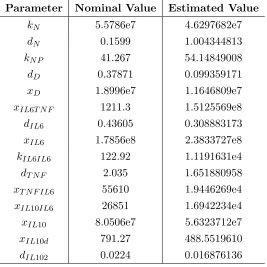
The optimized (estimated) values of the 21 parameters that defined 8D-21 are displayed in Table 3.4. The table shows that some of the free parameters optimized values were significantly different from their nominal values including kN P, kIL6T N F, xIL6T N F, kIL6IL6 and xIL10d. In addition, curve fitting plots of IL6(t), T N F(t) and IL10(t) for 8D-21 (red dashed line (- -)) and 8D (blue solid line (—)) are presented. The experimental data are represented by black circle (mean±SD) for the respective inflammatory cytokines.

(47)

Table 3.4: 8D-21 Model Parameter Estimation

Parameter Nominal Value Estimated Value

kN 5.5786e7 4.465195e7

dN 0.1599 0.54915952

kN P‡ 41.267 184.871881

kN T N F† 12.94907 22.7269753

kD 2.5247 4.63254241

dD 0.37871 0.15237897

xD 1.8996e7 2.620924e7

kCA 0.154625e-8 9.26423e-9

dCA 0.31777e-1 0.12553346

kIL6T N F† 4.4651 103.803383 xIL6T N F† 1211.3 1.504963e5

dIL6 0.43605 0.31720533

xIL6 1.7856e8 2.417754e8

kIL6IL6 122.92 2693.10339

dT N F 2.035 3.13284175 xT N F CA 0.19342 0.64397278 xT N F IL6‡ 55610 2.200224e6

xIL10IL6 26851 1.509456e4

xIL10 8.0506e7 6.900804e7

xIL10d‡ 791.27 5957.89231

dIL102 0.0224 0.01665673

†

Most identifiable only at dose level 3mg/kg ‡

Most identifiable only at dose level 12mg/kg

Figure 3.7 also depicted an excellent curve fitting plots for8D-21and8D at 3mg/kg(left plot) and 12mg/kg (right plot) endotoxin challenge levels, respectively. Both models (8D-21 and 8D) followed identical trajectories in predicting the experimental data onT N F(t) at 3mg/kg endotoxin level.

(48)

Figure 3.7: T N F(t) curve fitting plots comparing 8D-21 (- -) and 8D (—) against experimental data in black circle (mean±SD) at 3mg/kg and 12mg/kg endotoxin challenge levels; the plot on the left represents 3mg/kgand the right plot denote 12mg/kg.

(49)

increase the pool of models to compare.

3.4

7D Relative Sensitivity Ranking

In this section, we will redo the analysis that was carried out with the “modified 8D” models for the reduced 7D model.

(50)

Figure 3.9: 7D relative sensitivity ranking plots at 3mg/kg endotoxin level for IL6, T N F, IL10. The vertical dashed line in each plot indicate the cutoff point for the respective inflammatory response using the method discussed in Section 3.1.1.

(51)

kN 12 (0.1849) 3 (0.3927) 6 (1.7710)

xN 20 (0.0585) 6 (0.1363) 11 (0.7907)

dN 16 (0.1428) 4 (0.3210) 5 (2.4101)

kN P 24 (0.0427) 8 (0.1112) 15 (0.4563)

kN D 28 (0.0194) 20 (0.0416) 17 (0.3473)

xN T N F 29 (0.0181) 19 (0.0421) 19 (0.2430)

xN IL6 31 (0.0107) 28 (0.0225) 26 (0.1550) xN IL10 25 (0.0369) 10 (0.0858) 14 (0.5275) kN T N F 21 (0.0490) 7 (0.1142) 12 (0.6720)

kN IL6 30 (0.0129) 25 (0.0265) 24 (0.1866) kD 6 (0.3574) 12 (0.0732) 1 (5.4455)

dD 11 (0.2059) 17 (0.0472) 3 (4.4099)

xD 22 (0.0485) 30 (0.0120) 4 (2.6571)

kIL6T N F 17 (0.1128) 27 (0.0235) 30 (0.0822)

xIL6T N F 26 (0.0308) 32 (0.0062) 33 (0.0220)

kIL6 9 (0.3022) 14 (0.0629) 21 (0.2183) dIL6 8 (0.3170) 18 (0.0422) 28 (0.1111) xIL6 1 (1.2038) 5 (0.2504) 10 (0.8692) xIL6IL10 10 (0.3010) 15 ( 0.0627) 22 (0.2175) kIL6IL6 14 (0.1622) 21 (0.0337) 27 (0.1164) xIL6IL6 15 (0.1520) 22 (0.0317) 29 (0.1091) kT N F 23 (0.0463) 1 (0.4518) 18 (0.2434)

dT N F 27 (0.0283) 2 (0.4304) 25 (0.1796)

xT N F IL10 34 (5.44e-07) 34 (1.09e-05) 34 (3.57e-06) kT N F T N F 37 (1.2231e-15) 37 (1.92e-14) 37 (6.889e-15)

xT N F T N F 38 (1.2226e-15) 38 (1.91e-14) 38 (6.886e-15)

xIL10T N F 36 (3.79e-08) 36 (2.65e-09) 36 (3.40e-08)

kIL10IL6 18 (0.0947) 31 (0.0090) 31 (0.0530) xIL10IL6 7 (0.3232) 23 (0.0307) 23 (0.1885) kIL10 4 (0.4289) 24 (0.0280) 16 (0.3885) dIL10 3 (0.4996) 16 (0.0539) 9 (0.9496) xIL10 2 (1.0883) 13 (0.0714) 8 (0.9940) xIL10d