Computer Simulation and Analysis of Nanoparticle Delivery to the Olfactory Bulb for Direct Drug Migration to the Brain.

(1)

VACHHANI, SHANTANU AVINASH. Computer Simulation and Analysis of Nanoparticle Delivery to the Olfactory Bulb for Direct Drug Migration to the Brain. (Under the direction of Dr. Clement Kleinstreuer).

(2)

(3)

(4)

Drug Migration to the brain

by

Shantanu Avinash Vachhani

A thesis submitted to the Graduate Faculty of North Carolina State University

in partial fulfillment of the requirements for the degree of

Master of Science

Mechanical Engineering

Raleigh, North Carolina 2019

APPROVED BY:

_______________________________ _______________________________ Dr. Gregory Buckner Dr. Pramod Subbareddy

_______________________________ Dr. Clement Kleinstreuer

(5)

ii DEDICATION

(6)

iii BIOGRAPHY

Shantanu Vachhani was born on the 14th of May, 1995 to Mr. Avinash Vachhani and Mrs. Taruna Vachhani in Mumbai, India. After completing his high school education he attained his Bachelors of Engineering degree in the field of Mechanical engineering from Birla Institute of Technology and Science (BITS) Pilani, K.K Birla Goa Campus, Goa, India. Subsequently he moved to Raleigh, North Carolina in 2017 to pursue his graduate degree in Mechanical Engineering at North Carolina State University. He has been conducting research for his master’s thesis under the guidance of

(7)

iv ACKNOWLEDGMENTS

(8)

v TABLE OF CONTENTS

LIST OF TABLES ... viii

LIST OF FIGURES ... ix

CHAPTER 1. INTRODUCTION AND RESEARCH OBJECTIVES ... 1

1.1. Research Motivation ... 1

1.2. Literature Review... 2

1.2.1. Introduction ... 2

1.2.2. Nasal Drug Delivery Devices ... 5

1.2.3. CFD studies ... 10

CHAPTER 2. MATH MODEL DEVELOPMENT AND COMPUTER SIMULATIONS ... 15

2.1. Introduction ... 15

2.2. Assumptions ... 15

2.3. Airflow Equations ... 16

2.4. Particle Dynamics Equations ... 19

2.4.1. Drag Force ... 21

2.4.2. Brownian Force ... 22

2.4.3. Saffman Lift Force ... 22

2.4.4. Gravitational Force ... 23

2.5. Quantifying Particle Deposition ... 23

(9)

vi

CHAPTER 3. NUMERICAL METHOD USING OPENFOAM ... 26

3.1 Introduction ... 26

3.2. Case Structure ... 27

3.3. Case Set-up ... 34

3.4. Boundary Conditions ... 36

3.5. Numerical Schemes ... 39

3.6. Solution Control ... 41

CHAPTER 4. MODEL VALIDATIONS ... 42

4.1. Introduction ... 42

4.2. Geometry and Mesh of the Representative Nasal Cavities ... 43

4.3. Comparison with Calmet et al., 2018... 48

4.3.1. Airflow Field Results ... 48

4.3.2. Particle Deposition Results ... 54

4.4. Comparison with Ingham (1975) ... 57

4.4.1. Geometry and Mesh ... 57

4.4.2. Results and Discussions ... 58

4.5. Comparison with Tian et al., 2019 ... 60

4.5.1. Airflow Field Results ... 62

4.5.2. Particle Deposition Results ... 66

(10)

vii

5.2 Methodology ... 74

5.3. Results and Discussion ... 76

5.3.1. Micron-size Particles ... 76

5.3.2. Nanoparticles ... 85

CHAPTER 6. NASAL CANNULA FOR OLFACTORY DRUG TARGETING ... 95

6.2. Results and Discussion ... 97

CHAPTER 7. CONCLUSION AND FUTURE WORK ... 102

(11)

viii LIST OF TABLES

Table 2. 1. Boundary conditions for Particles. ... 24

Table 3. 1 Boundary conditions for Velocity and Pressure. ... 36

Table 3. 2 Boundary conditions for Turbulent Kinetic Energy and Turbulence Dissipation ... 37

Table 3. 3. Numerical Schemes used in simpleFoam. ... 40

Table 3. 4. Algebraic solvers used in simpleFoam. ... 41

Table 4. 1. Geometry features of the Nasal Cavity. ... 45

Table 4. 2. Unstructured mesh characteristics. ... 47

Table 4. 3. Comparison of particle deposition efficiencies. ... 54

Table 4. 4. Surface Area Comparison between G1 and G2 ... 62

Table 5. 1. Legend correlating the color to the specific region……….75

Table 6. 1. Olfactory deposition efficiencies for Cannula Injection (SOI = 10 m/s) ... 101

Table 6. 2. Olfactory deposition efficiencies for Cannula injection (SOI = 3.5 m/s) ... 101

(12)

ix LIST OF FIGURES

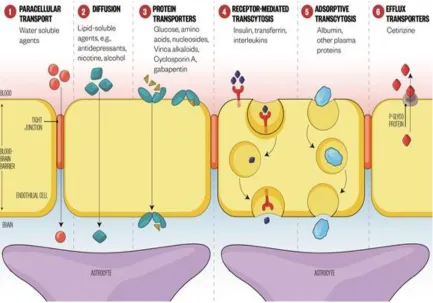
Figure 1. 1. Blood Brain Barrier (25). ... 5

Figure 1. 2. Anatomy of the Human Nasal Cavity (29). ... 6

Figure 1. 3. Schematics of a nasal spray (32). ... 7

Figure 1. 4. Schematics of a nebulizer (34). ... 8

Figure 2 .1.Workflow of Euler- Lagrange simulations...20

Figure 3. 1. OpenFOAM case structure. ... 28

Figure 3. 2. U file for the elbow case. ... 29

Figure 3. 3. boundary file in the polyMesh directory. ... 30

Figure 3. 4. transportProperties file in the constant directory... 31

Figure 3. 5. controlDict file in the system directory... 32

Figure 3. 6. fvSchemes file in the system directory. ... 32

Figure 3. 7. Workflow for conducting OpenFOAM simulations. ... 33

Figure 3. 8. transportProperties file. ... 34

Figure 3. 9. Snippet of the kinematicCloudProperties file. ... 35

Figure 4. 1. Geometry of the nasal cavity. ... 43

Figure 4. 2. Complete view of the Nasal Cavity Geometry. ... 44

Figure 4. 3. Isometric view of the unstructured mesh of the representative nasal cavity. ... 46

Figure 4. 4. Mesh slice of the mid-section of the nasal cavity... 47

Figure 4. 5. Mesh slice of the nostrils. ... 48

Figure 4. 6. Slices 1-1’ to 6-6’ (left to right) of the nasal geometry. ... 50

Figure 4. 7. Velocity contours (Slice 1-1’ and 2-2’). ... 50

(13)

x

Figure 4. 9. Wall Shear Stress contour of the nasal cavity for 20 lpm. ... 51

Figure 4. 10. Turbulent kinetic energy contour of the nasal cavity for 20 lpm. ... 52

Figure 4. 11. Particle Deposition Pattern for 2, 10 and 20 µm particles ... 55

Figure 4. 12. Sectional Deposition for 20 µm particles. ... 56

Figure 4. 13. Sectional Deposition for 10 µm particles. ... 56

Figure 4. 14. Cylindrical geometry. ... 57

Figure 4. 15. O grid meshing of the cylinder geometry. ... 58

Figure 4. 16. Deposition efficiency comparison for a flowrate of lpm... 59

Figure 4. 17. Deposition efficiency comparison for a flowrate of 5pm. ... 60

Figure 4. 18. Geometry G1. ... 61

Figure 4. 19. Geometry G2. ... 61

Figure 4. 20. Velocity contours along the nasal cavity for 5 lpm flowrate... 63

Figure 4. 21. Velocity contours along the nasal cavity for 10 lpm flowrate... 64

Figure 4. 22. Velocity streamlines across the nasal cavity. ... 65

Figure 4. 23. Velocity streamlines in the olfactory region. ... 65

Figure 4. 24. Recirculation regions in the nostrils……….66

Figure 4. 25. Dean vortices in the nasopharynx ... 66

Figure 4. 26. Deposition pattern for 10 lpm flowrate and 1nm diameter particle. ... 67

Figure 4. 27. TDE comparison for 5 lpm and 7 lpm flowrates. ... 68

Figure 4. 28. NOP Independent study for Total Deposition (10 lpm). ... 69

Figure 4. 29. ODE comparison for 5 lpm and 7 lpm flowrates. ... 70

Figure 4. 30. NOP Independent study for Olfactory Deposition (10 lpm). ... 70

(14)

xi

Figure 5. 1. Nasal geometry with the specific regions that will be represented in the ... 75

Figure 5. 2.1. PRM for an impaction parameter of 333.333 µm2cm3s − 1. ... 78

Figure 5. 2.2. Deposition efficiency comparison between normal and targeted injection. ... 78

Figure 5. 3.2. Deposition efficiency comparison between normal and targeted injection ... 79

Figure 5. 7. Deposition Pattern due to normal injection ... 83

Figure 5. 8. Deposition Pattern due to targeted injection ... 83

Figure 5. 9. Deposition Pattern due to targeted injection. ... 84

Figure 5. 11.1. PRM of 1 nm particles for the flowrate of 5 lpm. ... 86

(15)

xii

Figure 5. 17. Deposition Pattern due to normal injection ... 93

Figure 5. 19. Olfactory Deposition Efficiency trend due to targeted injection... 94

Figure 5. 20. Nasal Deposition Efficiency trend due to targeted injection. ... 94

Figure 6. 1. Streamlines to the olfactory region... 95

Figure 6. 2. Schematic of aerosol delivery using HFNC with a nebulizer.. ... 96

Figure 6. 3. Position of the injection of particles from the cannula. ... 96

Figure 6. 4.1. PRM of 2 µm particles for the flowrate of 20 lpm ... 98

Figure 6. 4.2. Deposition pattern as a result of cannula injection ... 98

Figure 6. 5.1. PRM of 10 nm particles for the flowrate of 20 lpm ... 99

Figure 6. 5.2. Deposition pattern as a result of cannula injection ... 99

Figure 6. 6.1. PRM of 50 nm particles for the flowrate of 20 lpm ... 100

(16)

1 CHAPTER 1. INTRODUCTION AND RESEARCH OBJECTIVES

1.1.Research Motivation

Brain tumors as well as Central Nervous System (CNS) disorders (Alzheimer’s, Parkinson’s, Multiple Sclerosis etc.) are major causes of fatalities in the world today. Malignant

brain tumors have a survival prognosis of less than 15 months (1) despite the progress that has been made. The most common brain cancer accounts for 80 % of all the malignant tumors (2). According to the Parkinson’s Prevalence Project, nearly 1 million American’s over the age of 45 will be diagnosed with Parkinson’s by 2020 and this number is expected to increase to 1.24 million by 2030. Alzheimer’s disease, according to the Alzheimer Association Report (2017), affects

nearly 5.5 million people and is the 6th leading cause of death in the USA. These statistics clearly underline the gravity of the situation. Therefore treatment of these diseases has garnered a lot of attention, and considerable efforts have been put into the treatment of these ailments.

(17)

2 transportation across the BBB. The blood cerebrospinal fluid barrier (BCSFB) forms the second layer that restricts the movement of drugs. This layer is located at the choroid plexus and separates the blood and the cerebrospinal fluid. However this layer is slightly more permeable than the BBB. The BBB surface area (120 sq ft) is roughly 5000 times the area of the BCSFB (6). Hence, BBB layer is the dominant obstacle for the delivery of drugs to the brain. These membranes are there to inhibit the passage of pathogens, antibodies, toxins etc. to the brain. In doing so they also restrict the transport of therapeutic drugs in to the brain. In summary, drug delivery to the brain is difficult to achieve at high enough efficiencies to counteract the toxins that are the root to the various CNS disorders (7).

1.2. Literature Review 1.2.1. Introduction

(18)

(19)

4 BCNU chip showed comparable efficacy to the BCNU polymerized wafer and further research should pave way for an encouraging future of microchip technology.

(20)

5

Figure 1. 1. Blood Brain Barrier (25).

1.2.2. Nasal Drug Delivery Devices

Drug delivery using the nasal route is a promising option and has been conventionally used in the form of nebulizers, nasal dry powder inhalers, spray pumps, nasal pressurized metered-dose inhalers, etc. Although the nose provides an accessible route to the olfactory region, there are certain challenge to nasal direct drug delivery (26-28).

(21)

6

Figure 1. 2. Anatomy of the Human Nasal Cavity (29).

(22)

7

Figure 1. 3. Schematics of a nasal spray device (32).

Metered-dose spray pumps have dominated the nasal drug delivery market since their inception. Figure 1.3 shows the schematics of a standard nasal spray. Standard spray pumps are associated with dose volumes between 25 and 200 µl. The components of a metered-dose pump spray are a container, the pump with a valve and an actuator. The dose spray characteristics like particle size are dependent on the orifice of the actuator, pump properties and the force exerted. Another device used for delivering nasal drugs is a nasal pressurized metered-dose inhaler (pMDI). A compressed gas is suddenly expanded resulting in a high speed release of the drug particles. However these are also associated with something called the “cold Freon” effect, characterized by discomfort and

(23)

8 m/s) (33) decreasing the irritation caused by the ‘cold Freon” effect. Until now, these pMDIs have not been used for nose-to-brain applications. A recent study is focused on developing a nitrogen-based inhaler but further in vitro and in vivo studies are required for practical implementation.

Figure 1. 4. Schematics of a nebulizer (34).

(24)

9 the respirable range. These nebulizers can also be used in conjunction with a high flow nasal cannula (HFNC). The HFNC efficiency has been analyzed (42, 43) for the purposes of ventilation and drug-delivery to lung sites. An in vitro study showed the maximum lung deposition efficiency of 32 % using this approach (44). The impact of gas flow and humidity using the nasal cannula in adults was studied by Alcoforado et al., 2019 (45). All the aforementioned studies have been concentrated on pulmonary drug delivery. Studies of direct nanodrug delivery to the olfactory bulb, using the cannula as an administering device, has not been published as the goal so far was to reach specific sites in the lung. For example, Longest et al., 2019 (46) reviewed the various nebulization technologies for delivering aerosols to the lungs and suggested secondary devices and technologies to increase the delivery efficiency of particles in the lungs. These claims are substantiated by the use of computational fluid dynamic simulations. Spence et al., 2019 (47) developed a new combination device with separate mesh nebulizers for generating humidity and delivering the medical aerosol. The device consists of a small volume mixing region where the aerosols are mixed with ventilation gas flow followed by a heating channel which produces small size droplets that are optimum for highly efficient nose-to-lung administration. Major utilization of these devices have been to target the sinuses and not the olfactory region. In addition to these liquid formulations, there are some powder formulations that are popular. These powder formulations are more stable than the liquid counterparts thereby eliminating the use of preservatives. These formulations are available in the market in three forms namely powder sprayers, powder inhalers and insufflators. Powder sprayers create a plume of spray particles due to the pressure created by the compressible compartment. Several studies (48-51) have been performed for testing the effectiveness of these devices in the market. On the other hand, nasal powder inhalers uses the subject’s breath to inhale

(25)

10 mouthpiece and a connected nosepiece. The subject exhales in to the mouthpiece, closing the velum which enables the airflow to carry the particles into the nosepiece.

1.2.3. CFD studies

(26)

(27)

(28)

(29)

14 during cyclic flows is lower than for steady flows. Furthermore the quasi – steady state assumption for transient flows is highly dependent on particle size, flowrate and breathing frequency. These factors can be combined to from the particle Strouhal number (Strp). A similar sniffing study for

(30)

15 CHAPTER 2. MATH MODEL DEVELOPMENT AND COMPUTER SIMULATIONS 2.1. Introduction

To conduct an accurate and realistic study of particle deposition in the olfactory region, it is essential to have the know-how of the underlying mathematical models to simulate the deposition mechanisms. This chapter provides the necessary equations and computer simulation approach in detail. The applicable conservation laws are difficult to implement, owing to the system’s high degree of complexity. Hence, to conduct successful Computational Fluid-Particle

Dynamics (CF-PD) simulations, certain assumptions have to be made which are listed in Section 2.2. After considering these assumptions, the resulting mathematical equations become simpler to solve. These equations are described in Section 2.3 along with the various particle transport forces which determine the trajectories of the particles. Chapter 3 then provides a brief introduction to the structure and working of OpenFOAM.

2.2. Assumptions

 The air inside the nasal cavity is taken to be an incompressible medium, indicating that there are no changes in the density of the air throughout the simulation. As the average human inhalation flow rate is between 15-20 lpm at approximately constant relative humidity, this is a reasonable assumption.

 All fluid dynamics processes are under isothermal conditions. Although there is always a

certain temperature difference between the body and the incoming air, this study is only concerned with the interplay of the flow-particle characteristics.

 Two-phase particle fluid simulations are characterized by fluid-particle interactions (one–

(31)

16 coupling). However because this study assumes that the fluid as a dilute suspension with volume fractions usually less than 10−3, only one –way coupling is considered.

 For the purposes of this study, the monodisperse droplets (or solid particles) are spherical

in shape. In this study, both nano- and micron- size particles are considered.

 Physiologically, the nasal cavity is lined with a mucus layer. The mucus layer is not

stationary and incorporation of this behavior into the simulation could be done by solving another complex boundary condition equation. Consequently the particle transport and deposition changes. However this is a very basic study and the effect of mucus layer will be considered in future works.

 In the case of droplets in the air, due to the heat transfer inside the nasal cavity resulting in

either evaporation or condensation, depending on the temperature difference. However since the study assumes isothermal conditions, these phenomena are not taken into account.

2.3. Airflow Equations

(32)

17 transitional regime with reasonable accuracy. Hence, unlike the laminar regime, the transitional regime is characterized by the flow transport equations in conjunction with the SST k- ω models. The Navier Stokes Equations

Continuity

∇. 𝒖 = 0 (2.1)

Momentum 𝜕 𝜕𝑡(𝑢𝑥) + (𝒖 . ∇)𝑢𝑥= − 1 𝜌 𝜕𝑝 𝜕𝑥+ 𝜕 𝜕𝑥[𝜈 ( 𝜕𝑢𝑥 𝜕𝑥 + 𝜕𝑢𝑥 𝜕𝑦 + 𝜕𝑢𝑥 𝜕𝑧)] + 𝑔𝑥 𝜕 𝜕𝑡(𝑢𝑦) + (𝒖 . ∇)𝑢𝑦 = − 1 𝜌 𝜕𝑝 𝜕𝑦+ 𝜕 𝜕𝑦[𝜈 ( 𝜕𝑢𝑦 𝜕𝑥 + 𝜕𝑢𝑦 𝜕𝑦 + 𝜕𝑢𝑦

𝜕𝑧)] + 𝑔𝑦 (2.2)

𝜕 𝜕𝑡(𝑢𝑧) + (𝒖 . ∇)𝑢𝑧 = − 1 𝜌 𝜕𝑝 𝜕𝑧+ 𝜕 𝜕𝑧[𝜈 ( 𝜕𝑢𝑧 𝜕𝑥 + 𝜕𝑢𝑧 𝜕𝑦 + 𝜕𝑢𝑧 𝜕𝑧)] + 𝑔𝑧

𝒖 denotes the velocity vector with 𝑢_𝑥, 𝑢_𝑦 and 𝑢_𝑧 as components of velocity along the x, y and z

directions. The pressure is denoted by 𝑝. The density and kinematic viscosity of the carrier fluid

are given by 𝜌 and 𝜈, respectively. The gravity force is represented as 𝑔𝑥 𝒊̂ + 𝑔𝑦 𝒋̂ + 𝑔𝑧 𝒌̂ .

As mentioned earlier, for transitional regime is modelled via the RANS equations which are given below.

𝜕𝑢̅̅̅𝑖

𝜕𝑥𝑖= 0 (2.3)

𝜕(𝜌𝒖̅̅̅)𝒋 𝜕𝑡 + 𝑢̅ 𝑖 𝜕 𝜕𝑥𝑖(𝜌𝒖̅̅̅) = −𝒋 𝜕𝑝 𝜕𝑥𝑗+ 𝜇 𝜕 𝜕𝑥𝑖( 𝜕𝒖̅̅̅𝒋 𝜕𝑥𝑖− 𝒖′̅̅̅̅𝑢′𝒋 𝑖)

̅̅̅̅̅_(2.4)

The velocity vector is represented by 𝑢_𝑗, where ‘j’ denotes the index. When the velocities in the

(33)

18 the fluctuating component (Eq. 2.5), it results in the formation of the RANS equations.

𝒖𝒋= 𝒖̅̅̅ + 𝒖′𝒋 𝒋 (2.5)

Where,

𝑢̅_𝑗= Average component of the velocity.

𝑢′𝑗 = Fluctuating component of the velocity.

When dealing with the RANS equations, it is extremely difficult to quantify the fluctuating component of the velocities because of their nature of randomness. Hence the shear transport term (𝒖′̅̅̅̅𝑢′_𝒋̅̅̅̅_𝑖) is modelled as shown in eq. This model formulation is based on the Boussinesq hypothesis

(1877).

𝒖′̅̅̅̅𝑢′𝒋̅̅̅̅ = 𝑣𝑖 𝑇( 𝜕𝒖̅̅̅𝒋

𝜕𝑥𝑖+

𝜕𝒖̅̅̅𝒊

𝜕𝑥𝑗) (2.6) As a result of the aforementioned modelling, RANS equations are no longer dependant on the fluctuating component of the velocity and hence solving the RANS equations is easier.To turn the RANS equations into a closed system of non-linear differential equations and make them solvable, it is necessary to obtain math models for 𝑣_𝑇 (known as the eddy or turbulent viscosity). In the current study, a SST-k- ω turbulence model is used to solve for the turbulent viscosity. This model approximates the turbulent viscosity as a function of the ratio of turbulent kinetic energy (k) and specific dissipation rate ω. This model is briefly explained below.

𝜕(𝜌𝑘) 𝜕𝑡 + 𝜕 𝜕𝑥𝑗(𝜌𝑢𝑗𝑘) = 𝑃̃ − 𝐷𝑘 ̃ +𝑘 𝜕 𝜕𝑥𝑗((𝜇 + 𝜇𝑡 𝜎𝑘) 𝜕𝑘

𝜕𝑥𝑗) (2.7)

where 𝑃̃_𝑘 and 𝐷̃_𝑘 are the terms for production and destruction of turbulence kinetic energy, respectively; 𝜇_𝑡 is the turbulent viscosity and 𝜎_𝑘 is the turbulent Prandtl number for k.

𝜕(𝜌𝜔) 𝜕𝑡 + 𝜕 𝜕𝑥𝑗(𝜌𝑢𝑗𝜔) = 𝛼 𝑃𝑘 𝑣𝑡 − 𝐷𝜔 + 𝑐𝑑𝜔 + 𝜕 𝜕𝑥𝑗((𝜇 + 𝜇𝑡 𝜎𝜔) 𝜕𝜔

(34)

19 where 𝜔 is specific dissipation rate, 𝑣𝑡 is the turbulent eddy viscosity, and 𝑐𝑑𝜔 is the cross

diffusion term.

𝜕(𝜌𝛾)

𝜕𝑡 + 𝜕

𝜕𝑥𝑗(𝜌𝑢𝑗𝛾) = 𝑃𝛾1− 𝐸𝛾1+ 𝑃𝛾2− 𝐸𝛾2+

𝜕

𝜕𝑥𝑗((𝜇 +

𝜇𝑡

𝜎𝛾)

𝜕𝛾

𝜕𝑥𝑗) (2.9) where 𝑃_𝛾1 and 𝐸_𝛾1 are transition source terms, 𝑃_𝛾2 and 𝐸_𝛾2 are destruction source terms and 𝛾 is

the intermittency coefficient. But since for calculating 𝑃𝛾1 we require critical Reynolds number

𝑅̃𝑒𝜃𝑐, a transported scalar 𝑅̃𝑒𝜃𝑡 is used in the transport equation to calculate 𝑅̃𝑒𝜃𝑐

𝜕(𝜌𝑅̃𝑒𝜃𝑡) 𝜕𝑡 + 𝜕 𝜕𝑥𝑗(𝜌𝑢𝑗𝑅̃𝑒𝜃𝑡) = 𝑃𝜃𝑡+ 𝜕 𝜕𝑥𝑗(𝜎𝜃𝑡(𝜇 + 𝜇𝑡 )𝜕𝑅̃𝑒𝜃𝑡

𝜕𝑥𝑗 ) (2.10) 2.4. Particle Dynamics Equations

An Euler-Lagrange approach was used to solve for the fluid-particle dynamics. Euler (in this case being the carrier fluid) refers to the fluid phase, being treated as a continuum, while the Lagrangian phase is being treated as a discrete phase (the drug particles). The Lagrangian phase is tracked individually along the particle path, where the particles are grouped together to form an “element” with the aggregation of such similar elements creating a control volume. The finite

volume methodology utilizes the control volume approach to solve for the scalar, vector and tensor fields associated with the carrier fluid. The particle transport equation for particles under consideration (micron and nano-sized particles) takes the form of Newton’s second law of motion.The workflow of equations solved in the Euler-Lagrangian approach in a particular time step is shown in Figure 2.1.The trajectories of the particles are calculated by time-marching the Ordinary Partial Differential Equations (ODEs) represented by Eq. (2.11).

𝑚_𝑝𝜕(𝒗𝒑)

𝜕𝑡 = ∑ 𝑭𝒑 (2.11)

(35)

20

Figure 2. 1. Workflow of Euler-Lagrange simulations. Euler Phase

3-D Navier-Stokes equations are solved using the finite-volume approach to calculate the various fields (velocity, pressure, etc.) associated with the fluid.

Lagrangian Phase Consequently these values are used to determine the various forces (Drag force, Brownian force etc.). These forces are used to time march the particle position via Newton’s second law of motion.

(36)

21 represents the summation of the various forces acting on the particle. The forces acting on the particle are greatly dependant on the size of the particles. For example, gravity and drag forces dominate the dynamics of micron particles while Brownian and lift forces play a major role in determining the trajectories of nanoparticles.

2.4.1. Drag Force

An important consideration for larger particles (micron size and above) is the drag force. The drag force is exerted on the particle due to its relative motion with respect to the fluid flow. It is dependent on the size and shape of the particle as well as the characteristics of the flow field. It is given by the following expression:

𝐹𝐷 = 1 2𝜌𝑣𝑟𝑒𝑙

2 _𝐶

𝐷𝐴𝑝 (2.12)

Where 𝜌 𝑖𝑠 the density of the fluid, 𝑣𝑟𝑒𝑙 is the relative velocity of the particle that is given by 𝑣 −

𝑣_𝑝 with the subscript p denoting the velocity of the particle. 𝐶_𝐷 is the drag coefficient that depends

on the particle Reynolds number (Eq.2.14) along the with Reynolds number of the carrier phase (74). A_p is the projected area of the particle which is given by Eq. (2.15).

𝐶_𝐷 = 24

𝑅𝑒 𝑘1(1 + 0.1118(𝑅𝑒𝑘1𝑘2)

0.6567_{) + 0.4305} 𝑘2 (1+ 3305

𝑅𝑒𝑘1𝑘2)

𝑘1 = 3

1+2ѱ−0.5

𝑘2 = 101.84148(−𝑙𝑜𝑔10 (ѱ)

)0.5745_(2.13)

ѱ (𝑠𝑝ℎ𝑒𝑟𝑖𝑐𝑖𝑡𝑦) = 1 (𝑓𝑜𝑟 𝑎 𝑠𝑝ℎ𝑒𝑟𝑒)

𝑅𝑒_𝑝= 𝜌𝑝𝑣𝑟𝑒𝑙𝑑𝑝

𝜇 (2.14)

𝐴_𝑝 = 𝜋

4 𝑑𝑝

(37)

22 2.4.2. Brownian Force

For particles in the nano-scale domain, corresponding to the ultra-fine suspensions in this study, the momentum is imparted to the particles by the fluid at random; unlike micron particles where inertia is the major driving force. As a result, the particles move in a random path. As the size of the nanoparticles increases, the influence of the Brownian force decreases. The Brownian force is given by the following equation.

𝑭_𝑩 = 𝜻√𝝅𝑺𝟎

𝚫𝒕 (2.16)

where 𝜁 is a zero-mean, unit-variance Gaussian random number , Δ𝑡 is the time-step size of particle integration and 𝑆₀ is the spectral intensity function defined as

𝑆₀ = 216 𝜇 𝑘𝑏 𝑇

𝜋2_𝑑 𝑝 5_𝜌

𝑝2 𝐶𝑐 (2.17) 𝑘𝑏 =

𝑅 𝑁𝑎=

8.315 𝑋 103 𝐽

𝑘𝑚𝑜𝑙 .𝐾

6.022 𝑋 1026𝑚𝑜𝑙𝑒𝑐𝑢𝑙𝑒 𝑘𝑚𝑜𝑙

1.38 𝑋 10−23 𝐽

𝑚𝑜𝑙𝑒𝑐𝑢𝑙𝑒 . 𝐾 (2.18)

here 𝜇 and 𝑇 is the dynamic viscosity and Temperature of the carrier phase respectively. 𝜇𝑝 and

𝑑_𝑝 denote the dynamic viscosity and diameter of the particle respectively. 𝑘_𝑏 (Eq. 2.18) is the Boltzmann constant and 𝐶_𝑐 is the Cunningham correction factor given by

𝐶𝑐 = 1 + 2𝜆

𝑑𝑝 (1.17 + 0.525 𝑒

−(0.78 𝑑𝑝_2𝜆 )

) (2.19)

𝜆 is the mean-free path of the carrier phase.

2.4.3. Saffman Lift Force

(38)

23 𝐹_𝐿 = 𝜋

6𝑑𝑝 3_𝜌𝐶

𝐿 ((𝑣⃗ − 𝑣⃗𝑝)Xcurl(𝑣⃗)) (2.20)

where

𝐶_𝐿 = 3 𝐶𝑙𝑑

2𝜋 √𝜌|𝑐𝑢𝑟𝑙(𝑣⃗⃗⃗)| 𝑑𝑝

2 𝜇

(2.21)

𝐶_𝑙𝑑 = 6.46 ∗ 0.0524 √0.5𝜌|𝑐𝑢𝑟𝑙(𝑣⃗⃗)| 𝑑𝑝 2

𝜇 (2.22)

2.4.4. Gravitational Force

Gravitational force is experienced due to the earth’s gravitational force. However for convenience Buoyancy forces are grouped with the gravitational forces. Buoyancy force is the upward exerted on the particle submerged in the fluid. These forces directly impact particle deposition due to sedimentation and hence for bigger particles it is essential to take these forces into account. It is given by Eq.2.23. The subscripts p and f represent the particle and carrier phase (fluid) respectively.

𝐹_𝑔 = 𝑚_𝑝𝑔 (1 −𝜌𝑓

𝜌𝑝) (2.23)

2.5. Quantifying Particle Deposition

For accurately determining the deposition efficiencies, it is essential to specify the various boundary conditions for the particles. OpenFOAM has three basic options, namely REBOUND, STICK and ESCAPE.

 The particle is said to STICK when it is at the particle-radius distance from the wall.

 REBOUND boundary condition makes the particle rebound from the particular patch

(Coefficient of Restitution = 1).

 The ESCAPE boundary condition allows the particle to pass through the particular patch

(39)

24

Table 2. 1. Boundary conditions for Particles.

PART BOUNDARY CONDITIONS

NASALINLET REBOUND

NASAL STICK

OUT ESCAPE

For an Euler-Lagrange approach, Deposition Fraction (DF) is a parameter used to quantify the percentage of deposition.

DFregion =

Number of particles deposited in a specific region

Number of particles entering the region (2.24)

2.6. Quasi-Steady vs Transient particle dynamics

(40)

25 steady state inhalation value that results in the same deposition as that of a transient case is calculated using the following formula :-

𝑄𝑚𝑎𝑡𝑐ℎ = 𝐶 (𝑄𝑚𝑒𝑎𝑛 + 𝑄𝑚𝑎𝑥 ) (2.22)

Where C ≈ 0.5 for all smooth inhalation forms.This result is an important one because it forms a

(41)

26 CHAPTER 3. NUMERICAL METHOD USING OPENFOAM

3.1 Introduction

For the purpose of this study, an open source Computational Fluid Dynamics toolbox named OpenFOAM (Open Field Operation and Manipulation) has been used (https://www.openfoam.com). In addition to being cost-free, this toolbox has far-reaching applications in engineering and scientific circles. Professionals from industry as well as academia utilize this toolbox to perform all facets of thorough Computational Fluid Dynamics activities, ranging from meshing (blockMesh and snappyHexMesh) to numerically solving 3-D complex flow systems (electromagnetics, turbulence, heat transfer, chemical reactions, multiphase flow, etc.). Owing to its open source nature, it facilitates the sharing of information and high level mathematical models for the purposes of a collaborative study. OpenFOAM is also highly compatible with various post-processing software (eg, ICEM, ParaView and Tecplot) and therefore results can be analysed without any inconvenience. OpenFOAM is built on the principle of Object Oriented Programming as it is written in C++. Therefore, all the models and computational solvers are built based on classes and objects. Furthermore, all the advantageous features of C++ (inheritance, encapsulation, data abstraction, etc.) are carried over into OpenFOAM, thereby making it quite user-friendly. The code structure is easy to grasp and enables the user to not only customize and extend the functionality of existing solvers but also to develop new ones with great ease. When dealing with numerical computations, running time is an important factor to be taken into consideration as certain computations may require months. Running these simulations in “parallel” has been shown to have reduced running (or computing)

(42)

27 multiple processors are simultaneously carrying out computations and exchanging data as opposed to only one processor solving necessary governing mathematical equations for the whole case geometry. OpenFOAM has built-in provisions for decomposition of cases, running them in parallel as well as reconstructing the decomposed fields for data analysing and post processing. It is essential to gain understanding of the unique case structure of OpenFOAM to make use of its full functionality. This structure is explained in the following section.

3.2. Case Structure

As mentioned earlier, OpenFOAM is a multi-purpose open source toolbox for carrying out computational studies (especially Computational Fluid Dynamics). It has various in built-in solvers with a sample case study associated with the solver. Each case directory in OpenFOAM has three main subdirectories: time directories, constant, and system. The content of these subdirectories varies from solver to solver. For example, the simplest solver in OpenFOAM is

icoFoam which solves the Navier-Stokes equations for an incompressible, isothermal system.

This case contains three subdirectories: 0, constant and system (Figure 3.1). The 0 folder is a time directory that holds the solution (in this case u and p for velocity and pressure, respectively) during the start of the simulation. Basically the 0 folder is used to specify the initial and the boundary conditions. These conditions can be very basic, such as a fixed value, to complicated ones like specifying a time-varying sinusoidal wave at the boundary via swak4Foam (Swiss Army Knife for FOAM). Like the 0 directory, there can be other time directories that stores

(43)

28

Figure 3. 1. OpenFOAM case structure.

For example, the tutorial case in icoFoam is simulating flow inside an elbow. The 0 folder of the elbow case requires the boundary conditions for pressure (p) and velocity (U). Figure 3.2 shows the U file for the elbow case. The file consists of the dimensions of the field, the internalField

which has the information of the initial conditions of the velocity and the boundaryField through which the boundary conditions are specified. In this case, the velocity magnitude is 0 throughout the internal mesh. Through OpenFOAM this field can be either uniform or nonuniform; wall-4, velocity-inlet-5 and pressure-outlet-7 are the names of the patches of the elbow geometry. Here, noSlip and fixedValue are examples of the Dirchlet boundary condition, while

zeroGradient is a type of Neumann boundary condition.The constant subdirectory has a polyMesh folder that contains the details of the mesh, ie, the number of points, boundary faces, neighbouring elements, etc. The directory constant, as the name suggests, also has the values of those properties that are not varying with time (eg, density, kinematic viscosity, etc.).

(44)

29

Figure 3. 2. U file for the elbow case.

the name of the various patches of the geometry along with the properties of the respective patches. The properties include the type of the part of the geometry, nFaces which gives the number of surface faces associated with that patch, and startFace which represents the number of the starting face cell of that patch. Apart from the boundary file, the polymesh directory contains other files namely cellZones, faces,faceZones,neighbour,owner,points and pointZones. For the purposes of solving the Incompressible Navier-Stokes equations (like the elbow case), the only fluid property required is the Kinematic viscosity. Figure 3.4 shows the

(45)

30

Figure 3. 3. boundary file in the polyMesh directory.

While icoFoam is a simple solver, other complex solvers require properties other than the kinematic viscosity. For nonNewtonianIcoFoam, the specific Non Newtonian Model (Quemada, Carreau, etc.) along with the value of specific coefficients while for conducting Computational Fluid-Particle Dynamics (CF-PD) simulations various parcel properties like parcel injection rate, number of parcels and parcel diameter are to be specified in the constant

directory.The system directory is comprised of three basic files namely controlDict,

fvSchemes and fvSolutions. The controlDict file is responsible for the Solution Time

(46)

31

Figure 3. 4. transportProperties file in the constant directory.

CFD involves discretizing non-linear mathematical equations into algebraic equations that are subsequently solved by certain matrix equation solvers. The process of discretization requires a lot

of accuracy and stability considerations and the fvSchemes file (Figure 3.6) allows you to choose a finite volume discretization scheme from an extensive list of available options that is most suitable for your particular study. Gradient, Divergence and Laplacian Schemes can be individually changed as per the requirement of the problem. Gradient, Divergence and Laplacian Schemes can be individually changed as per the requirement of the problem.

(47)

32

Figure 3. 5. controlDict file in the system directory.

(48)

33

Figure 3. 7. Workflow for conducting OpenFOAM simulations. Mesh

•Create the mesh in ICEM CFD and convert it into the OpenFOAM format using the command: fluentMeshToFoam

•Apply checkMesh -allGeometry -allTopology to detect for any bad elements and any other mesh quality parameters.

•As a result of these commands, a polyMesh folder detailing the points,cells,faces etc of the mesh is created.

Initial and Boundary Conditions

•The initial as well as the boundary conditions of all the fields (p,T,U,k,etc) are specificed in the 0 directory.

Properties

•The different properties that govern the simulation are specified in the constant directory.

•transportPropertiescontains the density and viscosity of the fluid which are necessary for solving the Navier-Stokes equations.

•turbulencePropertiescontains the specific turbulence model required to account for the turbulence effects.

•kinematicCloudPropertiesfile enables to specify the injection position, the parcel properties,etc.

Solution Control

•The next step is to specify the time step, write interval, etc in the controlDictfile present in the system directory.

•In addition to that the various finite volume schemes and the algebric solvers are specificed in the fvSchemes and fvSolutions files respectively in the same directory.

Running the Solver

•The final step includes running the respective solver. This can be done in two

ways:-•Serial - The simulation utilizes only one processor and hence is higher execution time. For e.g. running simpleFoamin serial processing is executed by the following command: simpleFoam.

•Parallel - OpenFOAM also has the option of running simulations using multiple processes. In this approach , the geometric mesh is decomposed into multiple parts where each processor is responsible for the

(49)

34 3.3. Case Set-up

As explained earlier, this study involves conducting one-way coupled fluid-particle dynamics simulations to determine the particle deposition efficiencies. The focus is on human nasal regions with an emphasis on the olfactory bulb for nanodrug migration across the BBB to the brain. This section underlines the case set-up for conducting this study. To conduct these one-way coupled simulations, the flow evolves first followed by conducting the particle tracking simulation using that flow field. OpenFOAM’s steady state, incompressible, turbulent solver

simpleFoam is used for conducting the steady simulations. Consequently, the convergent flow

field is used in icoUncoupledKinematicParcelFoam (OpenFOAM’s lagrangian solver) to keep track of the particles.

For solving the flow using simpleFoam, it is essential to specify the viscosity model as well as the density and kinematic viscosity of the fluid. Figure 3.8 shows the

transportProperties file used in the current study.

(50)

35 For icoUncoupledKinematicParcelFoam it is essential to determine the particle

properties will govern their trajectory. As mentioned these properties are specified using the

kinematicCloudProperties file. Figure 3.9 shows a snippet of the file to show the

syntax for providing information regarding the properties of particles, the forces acting on the particles and the injection model to be specified.

(51)

36 3.4. Boundary Conditions

It is essential to specify the boundary conditions for all the necessary flow and temperature fields to solve the necessary partial differential equations. In addition to the interior cells, the computational domain also consists of “ghost cells”. Ghost cells are layer(s) of cells that mirror

the boundary adjacent interior cells whose values are specified by these boundary conditions. The initial and boundary conditions of the pertaining flow-fields (velocity, pressure, velocity etc.) are set in the 0 folder.

There are three basic boundary conditions in the field of Computational Fluid Dynamics:

 Dirichlet: - When using a Dirichlet boundary condition, a particular value is assigned to the

variables at the boundary. e.g. 𝑢(𝑥) = 𝑐𝑜𝑛𝑠𝑡𝑎𝑛𝑡.

 Neumann: - When using a Neumann boundary condition, the gradient normal to the boundary is

specified for the variable. e.g. 𝜕𝑛 𝑢(𝑥)

= 𝑐𝑜𝑛𝑠𝑡𝑎𝑛𝑡.

 Mixed: - This is the mixture of the aforementioned boundary conditions and takes the following

form: 𝑎 𝑢(𝑥)+. 𝜕_𝑛𝑢(𝑥) = 𝑐𝑜𝑛𝑠𝑡𝑎𝑛𝑡.

Table 3. 1 Boundary conditions for Velocity and Pressure.

Boundary Velocity Pressure

Patch Type Syntax Type Syntax

NASALINLET Dirichlet fixedValue Neumann zeroGradient

NASAL No slip noSlip/fixedValue Neumann zeroGradient

NASOPHARYNX No slip noSlip/fixedValue Neumann zeroGradient

OUT Neumann zeroGradient Dirichlet fixedValue set

(52)

37

Table 3. 2 Boundary conditions for Turbulent Kinetic Energy and Turbulence Dissipation

Frequency.

Boundary Turbulent Kinetic Energy Turbulence Dissipation

Frequency

Patch Type Syntax Type Syntax

NASALINLET Dirichlet fixedValue Dirichlet fixedValue

NASAL Dirichlet kqR

WallFunction

Dirichlet omega

WallFunction

NASOPHARYNX Dirichlet kqR

WallFunction

Dirichlet omega

WallFunction

OUT Neumann zeroGradient Neumann zeroGradient

For a given boundary, different types of boundary conditions can be used for different variables. Table 3.1 shows the pressure and velocity boundary conditions while Table 3.2 shows the boundary conditions for the turbulence parameters: Turbulence Kinetic Energy and Specific Dissipation Frequency.The detailed description for the boundary conditions is given below:

{

type

<Boundary Condition Type>;

value

uniform <Specific Value>;

}

(53)

38

type is used to specify the name of the boundary condition recognized by the solver.

value, as the name suggests denotes the specific value (scalar or vector) of the boundary

condition.

The type options used in this particular study are as follows:-

 fixedValue:- This option maintains a particular value at the boundary patch. It is a type of

Dirchlet boundary condition. The value needs to be specified under the value option. E.g.

uniform (0 1 0) for a vector, uniform 2.0 for a scalar etc.

 noSlip:- This is special type of fixedValue boundary condition whose value is 0.

 zeroGradient:- This option indicates that the gradient of the variable normal to the boundary

is 0. It is a type of Neumann boundary condition.

𝛛𝐮

𝛛𝐧= 𝟎 (3.1)

u corresponds to the particular variable and n is the normal vector to the boundary patch.

As explained in Section 2.3, certain flowrates used for this study correspond to transitional regimes and hence it is essential to model the effects of turbulence. The existence of turbulence creates random fluctuations and as a result the velocity profile and wall effects are different from the laminar regime. A non-dimensional number 𝑦+(Eq) is used to divide the region near the wall into

three parts: viscous sublayer, buffer layer and log-law region.

𝒚+= 𝒖𝝉𝒚

𝝂 (3.2)

where 𝑢_𝜏 (eq) is the shear velocity , 𝒚 is the distance from the wall and 𝜈 is the kinematic viscosity

of the fluid.

𝒖_𝝉 = √𝝉𝒘

𝝆 (3.3)

(54)

39 Viscous Sublayer for y+ < 5

Buffer Layer for 5 < y+< 30 (3.4) Log − law layer for 30 < y+ < 200

𝑦+_{value can be thought of as a local Reynolds number and shows the relative significance between}

the turbulent and viscous stresses. Viscous Sublayer is the region closest to the wall where the laminar stresses are dominant. In the buffer region the stresses are of the same order while the log-law makes up >90% of the region where turbulence dominates. Due to its transitional nature, it is difficult to capture the flow-field physics of the buffer layer unlike the other two other layers.

Hence there is a need for empirical wall functions; for example, kqRWallFunction and

omegaWallFunction are options for the turbulence kinetic energy (k) and turbulent

dissipation rate (𝜔), respectively. These two turbulence parameters are essential to form a closed

system of turbulence equations that are required to resolve the flow completely. kqRWallFunction is a zeroGradient type of Neumann boundary condition. omegaFunction has a functionality of changing the value based on the y+ value.

The syntax for the aforementioned wall functions is similar to that of that of pressure and velocity. In addition to the initial and boundary conditions, the case set-up also requires the numerical schemes that are being used to solve the partial differential equations.

3.5. Numerical Schemes

(55)

40

Table 3. 3. Numerical Schemes used in simpleFoam.

Differential

Operation

Sub-Directory Variable Scheme Used

Divergence divSchemes

u bounded Gauss

linearUpwind

k bounded Gauss

limitedLinear 1

ω bounded Gauss

limitedLinear 1

ε bounded Gauss

limitedLinear 1

Temporal ddtSchemes u Euler

Gradient gradSchemes u Gauss linear

Laplacian laplscianSchemes u Gauss linear corrected

Interpolation interpolationSchemes u Linear

∇. 𝒖⏟ = 0 (3.5) ⃗⃗⃗

Divergence

𝜕𝒖⃗⃗⃗

𝜕𝑡⏟ + ( 𝒖⃗⃗⃗. ∇)𝒖⃗⃗⃗ = 𝑔 + 𝜇 𝜌 ∇

2_𝒖_⃗⃗⃗⃗

⏟ − 1

𝜌 ∇𝑝⏟ (3.6)

Temporal Laplacian Gradient

(56)

41 Table 3.3 shows the various numerical schemes used in the simpleFoam. These are mentioned

under the fvSchemes dictionary in the system directory. It also shows the sub-dictionaries corresponding to the differential operators. The finite-volume method solves for the average value of the system variables. However, the aforementioned numerical schemes require the values at the

boundary of each cell. Hence the need for the interpolationSchemes sub-dictionary. These schemes can be adjusted as per the requirements of the problem.

3.6. Solution Control

Table 3. 4. Algebraic solvers used in simpleFoam.

Variable Solver Smoother

U smoothSolver GaussSeidel

P GAMG GaussSeidel

K smoothSolver GaussSeidel

Ω smoothSolver GaussSeidel

Once the differential equations are converted into algebraic equations by the appropriate numerical schemes, certain algebraic solvers are used to get the values of the field variables at each time step. The choice of the solvers affects the computational time and stability of the simulation. Table 3.4 shows the algebraic solvers used for the system variables. GAMG (Generalized geometric algebraic

multi-grid) solver is used for pressure while the smoothSolver is used for the rest of the

variables. GAMG is a multi-grid solver and is considerably faster than the standard methods. This solver generates a quick solution for a coarser mesh, maps this solution onto the finer mesh and using it as an initial guess. The smoothSolver uses a standard Gauss Seidel approach to

(57)

42 CHAPTER 4. MODEL VALIDATIONS

4.1. Introduction

(58)

43 (mentioned in the fvSolutions directory) was achieved. Consequently, these field variables determined the values of the forces required for tracking the particle cloud.

4.2. Geometry and Mesh of the Representative Nasal Cavities

The geometry of the nasal cavity is shown in Figure 4.1. The figure depicts the nasal cavity and the nasopharynx. Furthermore, there is an extruded portion attached to the nostril to accurately simulate the inhaling action. Figure 4.2 shows the complete view of the nasal cavity from all angles. The complexity of the nasal cavity geometry is evident from these figures; thus, requiring proper care in generating the mesh. The nose geometry is constructed from the MRI scans of a healthy 53 year old, non-smoking male (weighing 73kg and 173 cm tall) provided by CIIT (Research Triangle Park, NC) (77-79).

(59)

44

(60)

45 Table 4.1 summarizes the various geometrical features of the geometry used. All the measurements are listed in MKS units. Particle deposition is subject-specific, i.e., variations in these geometrical features allow for comparisons between different patients. As a result, correlations can be established between these geometrical parameters and the particle deposition efficiencies.

Table 4. 1. Geometry features of the Nasal Cavity.

Geometry Features

Length 0.105

Height 0.093

Length/Height 1.129

Area 0.02280071

Volume 3.22981e-5

Area/Volume 705.945

Nostril Length 0.0111965

Nostril width 0.0040418

Computing with this geometry requires that mesh discretization is of high quality. To capture the intricacies of the computational domain, an unstructured mesh was created using ANSYS ICEM CFD (ANSYS Inc., USA). The procedure for generating the mesh is as follows:

 An octree-based method (80) was used in creating a high resolution surface mesh.

 The resulting surface mesh was then successively smoothened using Laplace smoothing

(81) to avoid shrinkage.

 Subsequently a Delaunay approach (82) was used to create a volumes mesh from the

(61)

46  Finally, prism layers were added to capture the boundary layers.

The final mesh is composed of tetrahedral elements in the core, prism elements along the boundary and pyramid elements in-between to have smooth transition between the elements. The cell size is highest in the core and lowest along the periphery. The finer prism cells serve to accurately capture the near wall physics and the turbulent characteristics of the flow. Due to the complex structure of the nasal cavity, repeated smoothing iterations were performed to ensure that the quality parameters, such as Aspect Ratio and Skewness, are of the minimum threshold required to obtain an accurate solution.

Figure 4. 3. Isometric view of the unstructured mesh of the representative nasal cavity.

(62)

47 with the aforementioned mesh.

Table 4. 2. Unstructured mesh characteristics.

Mesh Statistics

Number of Points 1071282

Number of Elements 4269286

Number of Faces 9106628

Number of prism elements 906380

Number of tetrahedral elements 3362856

Number of pyramid elements 50

Number of prism layers 4

Minimum edge length 3.08642e-06

Maximum edge length 0.00103895

(63)

48

Figure 4. 5. Mesh slice of the nostrils.

4.3. Comparison with Calmet et al., 2018

For model validation, the present results were compared to airflow pattern and particle deposition of Calmet et al., 2018 (60).This was done to confirm the validity of the Lagrangian micron-particle tracking approach used in OpenFOAM®. The paper presents a detailed analysis on the airflow and particle deposition efficiencies for varying flowrates (7.5lpm to 20lpm). Furthermore, a subject-variability study compared the velocity contours and deposition fractions between three different geometries. However, for the purposes of this thesis, only one representative nasal geometry has been considered, namely Subject A which is being used in this thesis.

4.3.1. Airflow Field Results

(64)

49 and the inlet flowrate is set to be at 20lpm. The velocity contours in each of these slices are given in Figure 4.7, where these are dimensionless velocity contours (u/Uinlet) perpendicular to the plane.

Furthermore, the dimensionless velocities of the first two slices range until unity and the rest of them range from 0 to 0.75. As it is evident from Slice 1-1’, higher velocities are observed in the left nasal cavity because of the smaller cross sectional area for the same inflow rate. The presence of these narrow, intricate pathways creates a jet- like flow. Slice 2-2’ shows the undulating pathway inside the nasal cavity. It also indicates that the bulk velocity is located in the middle where the superior portion receives zero flowrates.

(65)

50 stress is observed in the nasal valve. This is because the change in the direction of the flow directs the core of the flow closer

Figure 4. 6. Slices 1-1’ to 6-6’ (left to right) of the nasal geometry.

(66)

51

(67)

52

Figure 4. 9. Wall Shear Stress contour of the nasal cavity for 20 lpm.

(68)

(69)

54 4.3.2. Particle Deposition Results

4.3.2.1. Total Nasal Deposition

Figure 4.11 shows the particle deposition patterns for 2 µm, 10 µm and 20 µm spheres. As evident from this graphs, the nasal deposition is highly dependent on the particle diameter. Small particles follow somewhat the streamlines while larger microspheres with their inertia cross streamlines, thereby resulting in higher depositions (see Table 4.3). The slight discrepancy in the values may be due to the difference in the number of particles injected. The smaller particles go with the flow and escape through the nasopharynx, while the larger particles deposit inside the nasal cavity due to the dominating effects of inertia and secondary flows.

Table 4. 3. Comparison of particle deposition efficiencies.

Particle Diameter (µm) Total Deposition Efficiency % Simulations

Total Deposition Efficiency % Calmet et al. (2018)

20 98.5 97.9

10 53.37 55.65

2 3.32 3.12

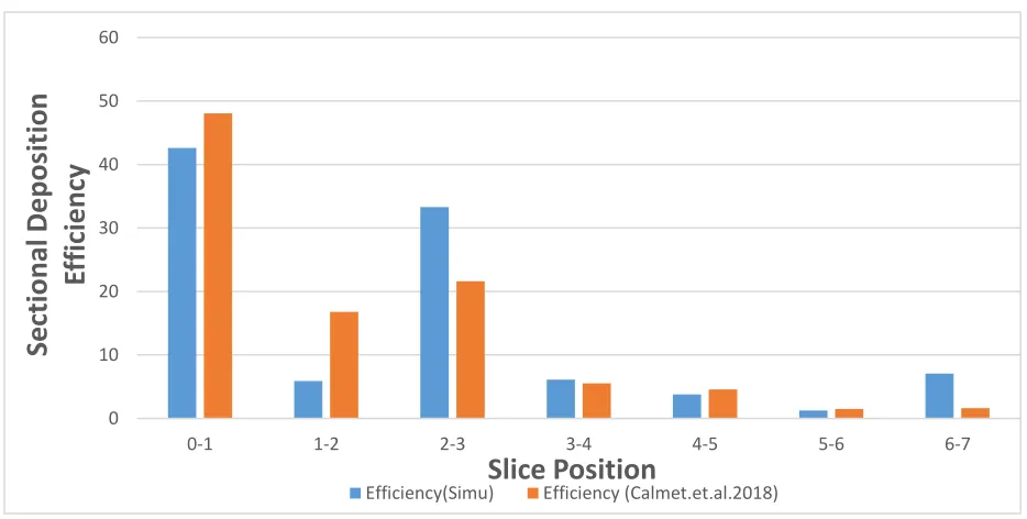
4.3.2.2. Sectional Deposition

(70)

55 Sectional Deposition Efficiency = Number of particles deposited in a particular section

Total number of particles inside the geometry

Figure 4. 11. Particle Deposition Pattern for 2, 10 and 20 µm particles (clockwise from the top).

(71)

56 It is also worthwhile to notice the similarities between the deposition pattern of 20 µm particles and the wall shear stress contour in Figure 4.9. The particle hotspots reasonably matched the high wall shear stress regions of the nasal cavity. Hence it can be concluded that for high inertial particles, hotspots are to be anticipated in the regions of high wall shear stress.

Figure 4. 12. Sectional Deposition for 20 µm particles.

Figure 4. 13. Sectional Deposition for 10 µm particles.

0 10 20 30 40 50 60 70 80

0-1 1-2 2-3 3-4 4-5 5-6 6-7

Secti

ona

l De

pos

it

io

n

Effic

ie

ncy

Slice Position

Efficiency (Simu) Efficiency (Calmet.et.al.2006)

0 10 20 30 40 50 60

0-1 1-2 2-3 3-4 4-5 5-6 6-7

Secti

ona

l De

pos

it

io

n

Effic

ie

ncy

Slice Position

(72)

57 4.4. Comparison with Ingham (1975)

Conventionally nanoparticles are tracked in the Eulerian frame rather than in the Lagrangian phase. However, the Eulerian approach is time intensive and does not offer a lot of flexibility as it pertains to parameters like injector position, number of injected particles, local deposition, site-targeting, etc. Furthermore, the Lagrangian approach offers a more realistic view of the fluid-particle dynamics inside the nasal cavity. In this section, the use of Brownian force, Cunningham drag force and the Saffman lift force (detailed in Section 2.4) for Lagrangian particle tracking of nanoparticles is validated by the analytical results presented by Ingham, 1975 (76). The particles are extremely small and are influenced by the process of diffusion. Typically the species-mass convection-diffusion equation has been employed for nanoparticles of dp<100nm. So, this

validation not only seeks to establish the accuracy of the solutions but also justifies the approach of using the Lagrangian approach for nanoparticle tracking. This Lagrangian approach has been validated in previous numerical studies as well (83, 84).

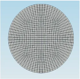
4.4.1. Geometry and Mesh

For this validation, a cylinder of diameter 0.0045m and length 0.09m was used, following Ingham (1975). The fluid-particle simulation was carried out with a finely structured mesh comprised of 673721 elements. The mesh was created using an O grid block. The geometry and the mesh used in the study is shown in Figure 4.14 and Figure 4.15, respectively.

(73)

58

Figure 4. 15. O-grid meshing of the cylinder geometry.

The flow in the pipe was fully developed laminar flow. The particles were distributed from the inlet as:

𝑚̇(𝑟) = 𝑚̇₀(1 −𝑟2

𝑅2) (4.1) Ingham (1975) presented the Deposition Efficiency (DE) correlation as follows:

𝐷𝐸 = 1 − (0.819𝑒−14.63∆+ 0.0976𝑒−89.22∆+ 0.0325𝑒−228∆+ 0.0509𝑒−125.9∆ 2 3 )

(4.2) where

∆ = 𝐷𝐿𝑝𝑖𝑝𝑒

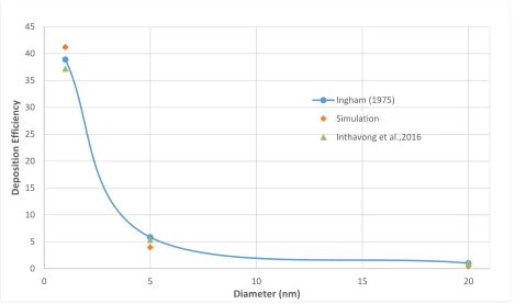
4𝑈𝑖𝑛𝑙𝑒𝑡𝑅2 (4.3) 4.4.2. Results and Discussions

(74)

59 studied for the flowrate of 1lpm (Figure 4.16) and 5lpm (Figure 4.17) which correspond to a Reynolds number of 312 and 1561 respectively. The numerical results are not only compared with the analytical solution as well as results presented by Inthavong et al., 2016 (83).

Figure 4. 16. Deposition efficiency comparison for a flowrate of 1 lpm.

As evident from the figures, the computer simulations closely resemble the analytical solution as well as the results presented in (83). The accuracy of nanoparticle deposition efficiency is dependent on the mesh size, the time step, and the number of particles injected. In this study 113,300 nanoparticles were injected and the time step of 1e-4 was used for time marching of the Lagrangian solution. The slight differences between the different studies can be attributed to the difference in the aforementioned parameters. The graph also illustrates that the larger the nanoparticle size, the lower is their dispersion and consequently a reduction in deposition efficiency occurs. Furthermore, nanoparticle deposition is inversely correlated with the flowrate. Higher flowrates imply stronger inertia and hence more particles are carried away by the flow in

0 5 10 15 20 25 30 35 40 45

0 5 10 15 20

D e p o si tion E ff ic ie n cy Diameter (nm) Ingham (1975) Simulation

(75)

60 the axial direction, restricting radial dispersion of the nanoparticles. This phenomenon is shown by the maximum deposition efficiency of 41 % in Figure 4.14 and 13.8 % in Figure 4.15.

Figure 4. 17. Deposition efficiency comparison for a flowrate of 5 lpm.

4.5. Comparison with Tian et al., 2019

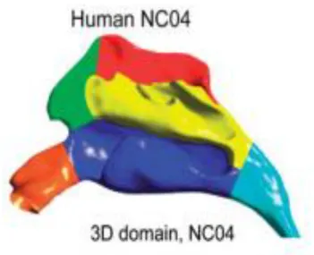
This section validates the nasal and olfactory deposition simulations for nanoparticles. Tian et al., 2019 (69) numerically analyzed the deposition of ultrafine particles (1 to 100 nm) under low and medium breathing rates for a realistic human nasal cavity. Nasal and olfactory depositions are highly subject-sensitive and before establishing any results, a comparison between the geometrical features needs to be done. G1 is the geometry used in the current study (Figure 4.18) and G2 (58) (Figure 4.19) is the geometry used by Tian et al. (2019). Table 4.4 compares the total and olfactory surface area of the nasal cavity between G1 and G2.

It can be seen from Table 4.4 that the area parameters for both the geometries are close and hence a comparative deposition study with the same range of flowrates can be done. However, Figures

0 2 4 6 8 10 12 14 16

0 5 10 15 20

D e p o si tion E ff ic ie n cy Diameter (nm) Ingham (1975) Simulation

(76)

61

Figure 4. 18. Geometry G1.

(77)

62 4.18 and 4.19 highlight the contrasting shape-features of these two nasal configurations. G1 has a narrow vestibule region as compared to the G2 geometry. In addition, a distinctive feature separating the two geometries is that G1 has a concave cavity separating the vestibule region and the nasal passages while G2 is characterized by a smooth transition between the vestibule and the airway passage. Apart from that, both the geometries have well-defined upper, middle and lower passages.

Table 4. 4. Surface Area Comparison between G1 and G2 in MKS units.

G1 G2

Nasal Cavity Surface Area .0196563 .019882

Olfactory Region Surface Area .00208761 .00194583

% of Olfactory to Nasal Surface Area

10.6 9.78

4.5.1. Airflow Field Results

Figures 4.20 and 4.21 show the sectional velocity contours for the in-house geometry, considering the sedentary breathing rates of 5lpm and 10lpm, respectively. It can be seen that both the flowrates have the same qualitative velocity contours. The air enters the nostrils in the vertical direction before accelerating in the vestibule region followed by deceleration inside the nasal cavity. Finally, due to the decrease in the size of the cross sectional area, the airflow accelerates into the nasopharynx.

(78)

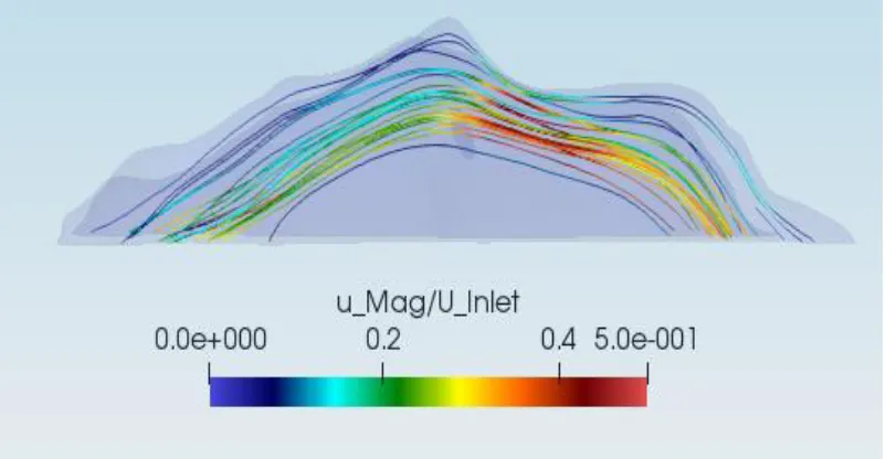
63 Figure 4.22 provides the streamlines and the respective velocity magnitudes throughout the nasal cavity. Since the study involves multiple flow rates (5, 7 and 10lpm) and all the flowrates lie in the laminar regime, the magnitudes are normalized with the inlet velocities. Ambient air enters the nostrils in the upward direction and turns 90 degrees entering the middle and inferior meatus before finally turning 90 degrees again towards the nasopharynx. Air enters the nostrils at a high velocity before decelerating inside the meatuses. It can also be seen that the olfactory region receives almost no air which is a major problem when it pertains to olfactory drug targeting. This phenomenon can be deduced from Figure 4.23.

(79)

64 After traversing through the meatuses, fluid accelerates into the nasopharynx due to the reduction in the cross-sectional area. It is also noteworthy to see the formation of recirculation zone formed around the nostrils (Figure 4.24). The nostrils are wider than the inlet that creates a low-pressure region resulting in the formation of the recirculation zone. Hence, it is reasonable to anticipate deposition of particles around the nostril region.

Figure 4. 21. Velocity contours along the nasal cavity for 10 lpm flowrate.

(80)

65 wall. In summary, most of the air inside the nasal cavity passes through the middle and inferior meatuses with very low velocities observed in the superior meatus closer to the olfactory region.

Figure 4. 22. Velocity streamlines across the nasal cavity.

(81)

66

Figure 4. 24. Recirculation regions in the nostrils Figure 4. 25. Dean vortices in the nasopharynx

4.5.2. Particle Deposition Results