A perturbation-based heuristic for the capacitated
multisource Weber problem
q
Z.M. Zainuddin
a, S. Salhi
b,* aMathematics Department, Universiti Teknologi Malaysia, Skudia, Johor, Malaysia
b
Centre for Heuristic Optimisation, Kent Business School, University of Kent, Canterbury, UK
Received 15 January 2004; accepted 15 September 2005 Available online 31 March 2006
Abstract
This paper proposes a perturbation-based heuristic for the capacitated multisource Weber problem. This procedure is based on an effective use of borderline customers. Several implementations are considered and the two most appropriate are then computationally enhanced by using a reduced neighbourhood when solving the transportation problem. Compu-tational results are presented using data sets from the literature, originally used for the uncapacitated case, with encour-aging results.
2006 Elsevier B.V. All rights reserved.
Keywords: Capacitated; Location–allocation; Continuous space; Heuristics
1. Introduction
The continuous capacitated location–allocation problem with a fixed number of open facilities each with a constant capacity, which is also known as the capacitated multisource Weber problem, may be stated as follows: given the location of each fixed point (customer point), the demand at each fixed point, the transportation cost for the area of inter-est, the number of facilities to open, and the capac-ity of each of these facilities, the aim is to determine
the location of each facility, and the allocation of customers to these open facilities (if more than one facilities are to be opened). Given
Parameters
n the number of fixed points (or customer
points)
wj demand or weight of customer j (j=
1,. . .,n)
aj¼ ða1j;a2jÞ location of customer jwhereaj2R2,
(j= 1,. . .,n)
M the number of facilities to be located
b fixed capacity of a facility whereb2N
Decision variables
Xi¼ ðX1i;X2iÞ coordinates of facility i where
Xi2R2
0377-2217/$ - see front matter 2006 Elsevier B.V. All rights reserved. doi:10.1016/j.ejor.2005.09.050
q
This research was conducted when both authors were at the University of Birmingham, UK.
* Corresponding author.
E-mail address:[email protected](S. Salhi).
xij quantity assigned from facility i to
cus-tomerj,i= 1,. . .,M,j= 1,. . .,n
The problem can be formulated as follows:
Minimise X
M
i¼1
Xn
j¼1
xijdðXi;ajÞ ð1Þ
subject to
Xn
j¼1
xij 6b 8i¼1;. . .;M; ð2Þ
XM
i¼1
xij ¼wj 8j¼1;. . .;n; ð3Þ
xijP0 8i¼1;. . .;M; j¼1;. . .;n; ð4Þ
whered(Xi,aj) represents the Euclidean distance
be-tween facilityiand customer j.
(1) denotes the objective function which is the
total transportation cost, (2) ensures that capacity
constraints of the facilities are not violated,(3)
guar-antees that the demand of every customer is satisfied
and(4)refers to non-negativity of the decision
vari-ablesxij.
It can be noted that once the set of open facilities has been decided upon (e.g., if we fix the open facil-ities in the formulation), the resulting problem reduces to the usual Transportation Problem (TP) which can be solved optimally in polynomial time. In short, the problem is to find the best facility configuration.
In this study the value of b is set to
Pn j¼1wj
M
wheredxeis the smallest integer larger than or equal
tox. Note that ifb> Pn
j¼1wj
M we introduce a dummy
customer with a 0 transportation cost and a demand
equals to the remaining demand, e.g., b
Pn j¼1wj
M .
This customer is used only when solving the TP, but not at the location and the allocation stages.
Most of the work in the literature on the capaci-tated facility location concentrates on the discrete problem and the methods mainly used include
dual-ascent based[11], cross decomposition method[13],
constructive-type heuristic [10,7] and Lagrangian
relaxation heuristics[2,1].
Other related work on the continuous location
problem include Eben-Chaine et al.[8]who studied
the case of capacitated facility location on a line,
and Brimberg and Mladenovic [4], Brimberg et al.
[3]and recently by Salhi and Gamal[12]who
inves-tigated the multisource Weber problem. To our
knowledge, it is only Cooper [6] in the 1970s who
attempted the capacitated continuous case. He pre-sented exact and approximate methods for solving the transportation-location problem. The heuristic method described in this work is a modification of
the alternating transportation-location method
introduced in [6]. Here, the location method and
the usual TP are alternately applied until there is no epsilon improvement in cost. We shall describe
Cooper’s method[6]as this will be used as the
foun-dation for our perturbation-based heuristic.
1.1. Cooper’s alternating transportation-location heuristic (ATL)
Firstly, M facilities are randomly chosen from
the fixed points. Then, the TP using these Mopen
facilities is solved to find the allocation for the
capacitated problem. For each of the M
indepen-dent set of allocations, containing ni fixed points
where i= 1,. . .,M and PMi¼1niPn, the new
loca-tion of the facilities is found using the iterative pro-cedure based on the Weiszfeld Equation which is given below:
X1iðkÞ¼
Pni
ji¼1
wjia1 ji
d Xð ðik1Þ;ajiÞ Pni
ji¼1
wji d Xð ðik1Þ;ajiÞ
and
X2iðkÞ¼
Pni
ji¼1
wjia2 ji
d Xð ðik1Þ;ajiÞ Pni
ji¼1
wji d Xð ðik1Þ;ajiÞ
; ð5Þ
where the superscriptk denotes the iteration
num-ber andwjirepresents all or a fraction of thejth
cus-tomer demand that is assigned to facility i.
Obviously wji6wj as some customers may have
their demand split because of the solution of the TP and hence some customers can be used more
than once in Eq.(5)with their appropriate demand
adjusted accordingly.
The location problem and the TP are alternately solved until there is no epsilon improvement in cost.
According to[6], ATL yields a convergent
mono-tone nonincreasing sequence of values for the objec-tive function. However, there is no guarantee that it will converge to the global minimum but the result, when not optimal, is found empirically to lie within
10%, and usually within 2–3%, of the optimal
solution when tested on small instances.
The rest of the paper is structured as follows: in the next section, the modification on
perturbation-based heuristic and section Section 4
presents a neighbourhood reduction for solving
the TP. Section 5 provides our computational
results and our findings as well as some research issues are given in the last section.
2. A modified Cooper’s heuristic
In this section we present a scheme for generating initial solutions and implementations that consider the diversity of these solutions when addressing the capacitated problem. These ideas with a slight modification within Cooper’s algorithm are then combined to form our first heuristic which we refer to as the modified Cooper’s heuristic.
2.1. The generation of an initial solution
The first part of the heuristic is to generate an ini-tial facility configuration. Instead of just starting
withMrandomly chosen points as in ATL, the
ini-tial facility configuration is found through solving heuristically the uncapacitated problem. This is used for two reasons (i) the solution found can be opti-mal or near optiopti-mal if found feasible, and (ii) this solution can be used as a lower bound especially if the solution is known to be optimal or very close
to optimal as shown in the literature (see [3]). Our
approach is based on Cooper’s multi-start alternate
algorithm (CMSA)[5]. For each starting
configura-tion, the Cooper’s alternate procedure of locate and allocate is carried out until there is less than epsilon improvement in cost, (say 0.0001). However, the solution found by this method is a local minimum. To increase the chance of getting a near optimal solution the method is repeated several times, say
K, using different random starting locations. In
other words, CMSA is the repeated use of Cooper’s alternate method.
2.1.1. The Furthest Distance Rule
The obtention of the initial solution can be car-ried out either randomly or via quick greedy heuris-tics for the p median problem. In our preliminary
testing (see [14, pp. 74–80]), based on the
50-cus-tomers problem from the literature (see[3]), we used
the multi-start heuristic as performed in Cooper, the Furthest Distance Rule which we refer to as the FDR, and also a combination of FDR and the drop heuristic. As a compromise between solution quality and computational effort we have opted for the FDR as our quick heuristic for generating our
ini-tial facility configurations for the uncapacitated location problem. The reasoning behind the FDR is to generate reasonably quickly initial facility loca-tion points which are situated far apart. This rule is defined as
X
i2E1
dðXi;ajÞ ¼max
j2J X
i2E1
dðXi;ajÞ; ð6Þ
whereE1is the set of facility locations already
cho-sen as initial points, J is the set of fixed points not
chosen yet, and (j*) is the new selected site using
Eq. (6).
The first point is chosen randomly from the
exist-ing fixed points, then the remainexist-ing M1 points
that are far apart are generated using Eq. (6). For
simplicity we restrict our initial location to a fixed point though this could be generated randomly in the plane. The algorithm that uses this idea is referred to as the Furthest Distance Method
(FDM for short) and its steps are given in Fig. 1.
2.2. Solving the capacitated location problem
In this section, we first discuss three implementa-tions based on the soluimplementa-tions found by the FDM to solve the capacitated problem, and then we present the algorithm which we refer to as the modified Cooper’s algorithm.
2.2.1. Multi-start alternate algorithm (MSA)
One way of solving the capacitated problem is by taking the best configuration (i.e., configuration
with the minimum cost) out of the Kruns for the
uncapacitated problem to be the starting configura-tion for the capacitated problem. In other words, the capacitated problem is only solved once.
2.2.2. Single-start alternate algorithm (SSA)
It is observed that, the best cost for the capaci-tated problem does not necessarily originate from the initial solution that yields the best cost for the uncapacitated problem. Therefore, another way of
solving the problem is by considering all theK
con-figurations for the uncapacitated problem to be the initial starting location for the capacitated problem.
In this case, the capacitated problem is solved K
times.
2.2.3. Intermediate-start alternate algorithm (ISA)
In this method, the capacitated problem is solved by using a sample of configurations extracted
configurations, D<K) obtained when solving the uncapacitated problem. The scheme of selecting
these D configurations is described below. Once
theseDconfigurations are chosen, we will then
pro-ceed to solve the capacitated problem for each value
of theseDscenarios. This scheme could be seen as a
compromise between the MSA and the SSA. For
instance, if D=K, this becomes the SSA whereas
whenD= 1 it is the MSA. It is obviously clear that
when the value of D gets larger, the quality of the
solution when solving the capacitated problem gets better or remains unchanged but such a gain in quality requires relatively more computing time.
In this paper, the diversity or the dissimilarity of the sample candidates is measured based on the
cost. TheKconfigurations are arranged in
ascend-ing order of the cost. The least cost configuration (i.e., the top of the list) is always selected since it has the minimum cost. To choose the other
(D1) candidates, the gaps between two successive
costs are calculated and used as a measure to differ-entiate between dissimilar configurations. In this approach we only consider the configurations with
gaps larger than a prescribed gapwhich is defined
as the average value of the gaps, i.e., ¼
PK1 t¼1GðtÞ
K1
where G(t) represents the gap between the cost of
Fig. 1. The Furthest Distance Method (FDM).
the (t+ 1)th and thetth configuration. Thus, in this
scheme, the value ofDis not necessarily constant.
2.3. The modified Cooper’s algorithm
The capacitated problem is solved using a proce-dure modified from Cooper’s ATL. This method which we refer to as the alternating transporta-tion-location–allocation-location method (ATLAL) is similar to the ATL except that instead of alternat-ing between the TP and the location problem, we
add another step (see step 4 in Fig. 2) where after
we get the new location of the facilities, we allocate the customers to their nearest facility, solve the loca-tion problem again and then the TP for the new allocation for the capacitated problem. The main
steps of ATLAL are given in Fig. 2, for a given d,
d= 1,. . .,D where D= 1,K or 1 <D<K. Let Sd
be the dth configuration and cost(Sd) its
corre-sponding cost. Ifd> 1, we select the configuration
yielding the overall least cost, costðSdÞ ¼
mind¼1;...;DfcostðSdÞg.
We would like to note that the introduction of this additional step (step 4) no longer results in a convergent sequence as the monotonic property can be lost from one cycle (step 2 to step 5) to another. However, this shake up is embedded pur-posely to provide flexibility in exploring more than one local minimum by being able to escape from regions of the previously found local minima.
3. A perturbation-based scheme
A post optimisation procedure that attempts to improve the currently found solution by ATLAL
for each Sd, d= 1,. . .,D is proposed. In this
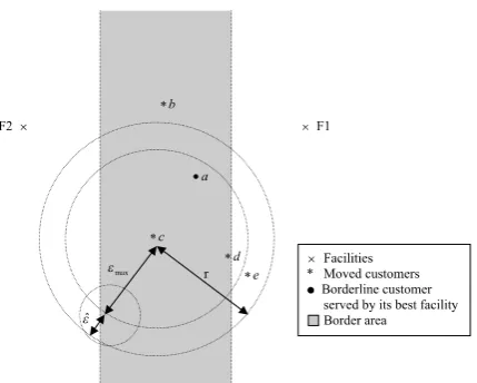
approach, the locations of the facilities found with the ATLAL heuristic are perturbed by taking into account the clustering of the borderline customers. These customers are defined as those which lie in between their nearest facility and their second near-est facility. In other words, the distance between the customers and their nearest and second nearest facilities is more or less the same. The formation of these clusters is defined in the next subsection. The point candidates (customers) of these clusters are temporarily forced to be assigned to their near-est facilities while we solve the TP. This task is per-formed by temporarily removing these customers from the system when we are solving the TP and then re-introducing them back when we solve the location problem. This restriction is imposed in
order to make the locations of their ‘best’ facilities nearer to these customers. When using these new locations, it is likely that some of these customers will be allocated to their nearest facility as in the uncapacitated case. This scheme is repeated starting with the recent best configuration for the capaci-tated problem until there is no epsilon reduction in cost or when there is no borderline customers that can be served by their second best facility. The remainder of this section covers the different mecha-nisms used within this perturbation-based procedure.
3.1. The creation of the clusters
The construction of the clusters is performed as follows:
3.1.1. Borderline customers
We identify the set of borderline customers, B,
irrespective of the capacity of the facilities as
B¼ i2 f1;. . .;ng s.t.qi¼
dðF1;iiÞ
dðF2;i;iÞ Pqmax
;
where d(F1,i,i) is the distance of customer i to its
nearest facility, F1,i,d(F2,i,i) is the distance of
cus-tomer ito its second nearest facility,F2,i, andqmax
is the cut off point.
The choice of the valueqmax is important. If the
value is too small (near 0), too many points will be
in the setBand if it is too large (near 1), the number
of points in B will be too small. In this work, the
value ofqmax is found dynamically as shown below
where the initial value ofqmax is set to 0.8.
3.1.2. Assignment of customers
The set of customers that were re-assigned not to
their nearest facility, due to the TP, is defined byB1as
B1¼ fi2Bandiis not completely allocated toF1;ig
¼ fjhgh¼1;...;H;
whereHdenotes the number of elements inB1(i.e.,
jB1j).
Note that B1may include borderline customers,
that are not necessarily served by the second,
third,. . ., best facility. Note also if the weight of a
customer is not unity, this customer may be served by more than one facility. In this case, even if a frac-tion of the weight of some facility is served by its ‘best’ facility, it is still considered as a candidate in
explana-tion on this issue will be given in Secexplana-tion 3.1.3
below.
(a) CaseB1= {} (i.e., all the borderline customers
are completely served by their ‘best’ facility).
• If qmax>qmin (the minimum cut off, say
0.6), do the following steps:
Do whileqmax>qmaxmin andB1= {},
setqmax=qmax0.1 and reconstructB1
Enddo
• If qmax=qmin (i.e., all the borderline
cus-tomers are still served by their ‘best’ facil-ity), do the following;
if(the perturbation scheme is applied for the first time)then
take the configuration found for the capacitated problem using ATLAL with-out the perturbation scheme.
else
take the best configuration found from the previous application of the perturba-tion scheme as the best soluperturba-tion.
endif
(b) CasejB1j> 0 (i.e., not all borderline customers are completely served by their best facility).
Setqmax=qmax0.1, reconstructB1, and let
L=jB1j.
if (L>H) take the new value of qmax and
the new setB1.
else(i.e.,L=H) take the previous value of
qmax and the previous setB1since there is no
change in the number of candidates ofB1even
withqmax decreased.
endif
The last value of qmaxfound is then used as our
cut off point for generating borderline customers.
Note thatLPH.
3.1.3. Formation of the clusters
AfterB1has been identified, we proceed with the
formation of the clusters. The maximum number of
clusters is taken to be k0, which is set to Min our
study. We first find the centres of the clusters then assign the customers to these clusters.
(a) The obtention of the centres of the clusters
• Find X1 the centre of the cluster C1 such
that X12B1. The first centre is chosen as
the customer of B1with the smallest value
ofqi.
• Apply the Furthest Distance Rule as given
by Eq. (6) based on B1 to get the other
k01 centres,Xk2B1,k= 2,. . .,k0.
The idea of using the Furthest Distance Rule in finding the centres is that we want the centres to be as far away from each other as possible. This is because, if the cen-tres are too close to each other, they may attract one another in the process of clus-tering the points.
• Construct a forbidden region
Note that, when applying the Furthest Dis-tance Rule we may get a point which is close to one of the points we have already selected previously. To avoid this, we impose a forbidden region around the cur-rent centre/s. The concept of making previ-ously visited solutions forbidden for future exploration is one of the key factors in tabu search meta-heuristic methodology. In this work, for simplicity, we define such a region by a circle centred at the current cen-tre with a radius to be defined below. In other words, only the points that are out-side the already constructed circle(s) are potential points for cluster centers. There-fore, the number of clusters may be less
than or equal to k0, say k1. A similar idea
was also used by Gamal and Salhi[9]when
solving the multi-source Weber problem. The radius of the forbidden region is defined as follows. Initially, the customers situated within a certain radius around the centre are found. As there might be some other points that lie close to these already chosen customers but happen to be just marginally outside the cluster, the neigh-bouring customers of these chosen points need also to be included in the cluster. In the following, for simplicity of notation, we consider the first cluster as an example since the same formulae applies to all the
kclusters. Let d(X1,FX1) be the Euclidean
distance between the first centre X1 and
the facility that serves it (FX1) and set the
radius of the forbidden region (r) to
r¼maxþ^where max is the initial radius
set todðX1;FX1Þ
2 . In other words, customers
sit-uated within this radius of the centre will be assigned to this cluster.
^is the radius of the neighbourhood of the
dðX1;FX1Þ
4 . This flexibility is introduced to
allow those customers very close to those
already assigned based on max to be
included.
(b) The generation of the clusters
Let B2be the set of all customers served by
other facilities than their best one and note
that B2 is not necessarily a subset of B1.
Fig. 3 shows how r, max and ^ are defined
for a given cluster k, and also illustrates the
elements inB,B1,B2and the clusterCk. For
each centre, those customers inB2which fall
within the radiusmaxare checked. If the
clus-ter is empty (this means that there are no other candidate besides the centre), then the next centre is checked and so on. If some customers are obtained, the cluster’s candidates are assigned as follows. Firstly, those customers
which fall within the radius are assigned to
the cluster, initially =min, see Fig. 4 for
details. If the cluster is empty, the value ofe
is increased by a fixed amount (say b= 0.1)
up to max until customer(s) are assigned to
this cluster. Then, the neighbouring customers
which lie outside the radius but withinmin
radius of the currently chosen customers are also chosen. To obtain the cluster’s candidates
for a certain cluster, say clusterk, the scheme
given inFig. 4can be followed.
Note that if some customers are served by their ‘best’ facilities, even though they are located close
to one another, as in a cluster, they will not be con-sidered to form a cluster.
3.2. Temporary removal of clusters
In this subsection, we restrict the clusters to remain assigned to their nearest facility while we solve the allocation problem. Note that as the total demand of those customers in a given cluster is rel-atively smaller compared to the capacity of the
facil-ity as given by the value of b, the assignment of a
given cluster to its nearest facility is therefore feasi-ble. In the case where the facilities happen to have different capacities, the proposed relaxation scheme needs to be modified to cater for such a situation. In this scheme we temporarily omit the customers of the clusters when we are solving the TP. By doing this, we are forcing the customers to remain served by their nearest facilities until the location of the facilities become unchanged from one iteration to the next. However, if by assigning a cluster point to its nearest facility violates the supply constraint of that facility, the point will be omitted from the cluster. This is repeated for all the clusters obtained.
The main steps are summarised inFig. 5.
We present two variants for handling these clus-ters when solving the TP with full capacity. The issue here is to avoid the snowball effect where the location and allocation of one facility will affect the location of other facilities and the allocation of their customers. The first variant is based on tem-porarily removing all clusters one at time whereas the second concentrates on temporarily removing only those clusters that are likely to have an effect on the total cost.
3.2.1. Removal of all clusters
The location and their allocation problems with full capacity are solved alternately for all the clus-ters until less than epsilon improvement in cost is found. Obviously, this will require relatively a
longer computing time since there are k1 full TPs
to be solved at each iteration.
3.2.2. Removal of some clusters
An empirical study is conducted to see the impact of the change after solving the TP without those customers belonging to the clusters (step 3 of
Fig. 5), (dL)k wherek= 1,. . .,k1 to the final solu-tion found by the full TP when using the final
con-figuration. This change in cost (dL)k is then sorted
in descending order. It is worth noting that in some Fig. 3. Formation of a given clusterk,k= 1,. . .,k1with radiusr
instances, the final solution is found to be better
even though the respective change in cost (dL)k is
lower. Therefore, the difference between the highest
change in cost (dL)1 and the change in cost (dL)k
that yields the best solution is calculated for 2–25 open facilities for the 50-fixed points problem and the 287-fixed points problem. These data sets which are usually used for the multisource Weber problem
are taken from the literature (see[3]). From this
lim-ited preliminary experiment, we observed that it is
not necessary to solve the full TPs for all the clusters but only to concentrate on those clusters having a change in costj(dL)kj64j(dL)1j. Here, at iteration,
the number of full TPs solved isk2wherek2k1.
This simple but powerful reduction scheme will then be used in our future testing.
In this approach, we explore another
configu-ration besides the k2 configurations already
obtained. We restrict to just one more only to pro-vide more flexibility while limiting the additional Fig. 4. The selection of thekth cluster candidates,k= 1,. . .,k1.
computational burden as this exercise is performed
for each value ofd (d= 1,. . .,D) and at each
itera-tion. It may be useful to investigate the effect of exploring more than one additional configuration in future. The idea is inspired from Genetic Algo-rithms where a new solution is constructed based on combining two existing configurations. Here,
only the clusters with positive (dL)kare considered
for combination. The rational behind this is that if we combine two or more clusters having positive
(dL)k values, we may generate a new solution with
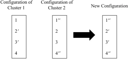
a higher positive value. The new configuration will take the location of the affected facilities of all the
clusters involved. For instance, inFig. 6 where we
have two clusters and four facilities to be opened, after temporary removing the cluster candidates, the location of facilities 2 and 3 are changed in clus-ter 1 and the location of facilities 1 and 4 are chan-ged in cluster 2. Therefore, the new configuration will take the location of facilities 2 and 3 from ter 1 and the location of facilities 1 and 4 from clus-ter 2. However, if there are shared affected facilities, the location of the facilitiesi,i= 1,. . .,Mwith more
total demand will be taken. For example, inFig. 7,
the location of facility 3 is changed in both clusters 1 and 2. But, since the demand to facility 3 at the loca-tion in cluster 1 is more, or in other words, facility 3 has more customers if it is situated as in cluster 1, therefore, the new configuration will take the loca-tion of facility 3 from cluster 1. At each iteraloca-tion, the number of full TPs to be solved in this method
is thenk3=k2+ 1.
The selected configuration is the one that yields the least cost after solving the full TPs in both clus-ter methods.
As the solution obtained might be a local mini-mum, the perturbation scheme is then applied with the recently chosen configuration as the starting locations. However, before doing this, the change between the current cost of the capacitated problem
after applying the perturbation scheme, cap*(S
d),
and the cost of the capacitated problem without
the perturbation scheme, cap(Sd), is evaluated. Let
(dG)ddenote this change.
• If (dG)d is positive, we start the perturbation
scheme again with the recently obtained configu-ration.
The process of creating the clusters, forcing them to stay at their nearest facilities and solving the location and allocation problem is repeated until
there is less than reduction in cost. It can be
observed that after a few iterations, though the number of clusters and the candidates of the clus-ters remain the same, we still continue with this process until no more improvement in cost. We adopt this strategy since the location may have changed without affecting any change in the allocation.
• IfdGdis negative, we record cap(Sd) as our
solu-tion and stop.
4. Effect of neighbourhood reduction
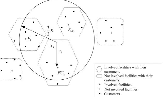
It can be shown that a large amount of the total cpu time is consumed in solving the large number of TPs. Note that though the TP is solved in polyno-mial time, the use of such a procedure so many times renders the whole exercise computationally unattractive. There are a few ways on how to over-come this drawback. In this study, at each iteration, when solving the TP, we concentrate on a smaller portion of the original problem by considering a subset of facilities only. A smaller neighbourhood is then defined and the TP is solved for the facilities involved and their respective customers only. The
main steps of the procedure are given in Fig. 8
and an illustration is provided in Fig. 9. In other
words, for each cluster, we determine those facilities close to it and the assigned customers and then solve the TP based on this smaller subset of facilities. ′
′
′′
′′ ′′
′
′
′′
Fig. 6. No shared affected facilities.
′
′ ′′
′′ ′′
′
′
According toFig. 8, we apply the TP based onjH*j facilities (jH*j<M) andA(H*) the new set of
allo-cated customers instead of n where jA(H*)j<n.
Note that the selection of neighbourhood is carried out using a distance-related criterion but other pro-cedures such as the use of the Voronoi diagram are also possible. Though the latter scheme may obvi-ously select more precisely those affected facilities, since the process of alternating between location– allocation requires several iterations, our approxi-mation scheme in detecting the affected facilities is reasonably appropriate. This reduction scheme is embedded into our method when we are solving
the TP for Mtimes while temporary removing the
cluster’s candidates. The effect of such a reduction is demonstrated in our computational results in the next section.
5. Computational results
The proposed heuristics are written inFortran90
and run on Sun Enterprise Workstation 450 run-ning Solaris 2.6. We used the four test problems given in the literature for the uncapacitated case,
see[3]. These are the 50-fixed points, the 287-fixed
points, 654-fixed points and the 1060-fixed points test problems. The weight of all customers is set to unity except for the 287-fixed point problem. The algorithms are applied to the test problems to solve for 2–25 open facilities for the 50-fixed points prob-lem and 5–50 with an increment of 5 for the other three problems. To evaluate the performance of our heuristics, we present the computational results obtained when solving the problem using the ATL and the ATLAL.
Fig. 8. Definition of a smaller neighbourhood (jH*j<M,jA(H*)j<n).
As these instances do not include the capacity of the facilities, we generate the capacity of the facility
asb¼
Pn j¼1wj
M
. The value ofbis for some facilities
either larger or smaller than the total demand of the allocated customers to the facilities for the case of the uncapacitated problem. Note that in some cases, the total supply of the facilities will exceed the total customers demand as we are using the smallest
inte-ger which is greater than
Pn j¼1wj
M . In this case, a
dummy customer with a unit transportation cost of 0 and a demand equals to the remaining demand is added. This dummy customer is used only when solving the TP, but not at the location and alloca-tion stages.
The values of the parametersKandare found
empirically using limited experiments. These include
K= 50 as required in Fig. 1, and = 0.0001 as
referred in several places throughout the text. We compute the % deviation based on the cost found for the multisource Weber problem. As these solutions were already reported in the literature to
be optimal or very close to optimal (see [3]), we
can therefore use such solution costs as lower bounds in our experiments. These are the optimal solutions for the 50 and 287-fixed points problems and the best known solutions for the 654 and
1060-fixed points problems given in[3]. The
devia-tion is then computed based on these lower bounds as follows:
devð%Þ ¼FbestFLB
FLB
100;
whereFbestis our overall best solution cost andFLB
refers to the lower bound or ‘best’ cost for the unca-pacitated case. We also record the overall average deviation (OAD) for the instances for each of the four test problems.
We conducted two experiments. In the first one, our aim is to select, based on the smallest data set, the most appropriate cluster type method which will then be used in our second experiment. This variant is then used with the reduction neighbourhood when dealing with the larger data sets.
5.1. Experiment 1: The choice of the variant for the large capacitated problems
The decision is based on the solution quality (measured by the average deviation) and the aver-age computing time for the SSA, MSA and ISA
using the all-clusters method (A: single all cluster, B: multi all cluster and C: intermediate all cluster, respectively) without the neighbourhood reduction for the 50-fixed point problem. These three algo-rithms are applied to solve for 2–25 open facilities. The average deviation obtained through SSA was 10.20% using 23.67 seconds of computing time, 13.11% through MSA with 0.81 seconds and 10.21% through ISA with 9.10 seconds. The detailed
results of all the test problems can be found in[14].
According to our limited experiments, ISA gives much lower average deviation than MSA but a frac-tion higher than SSA. In terms of computing time, ISA takes much shorter time than SSA but slightly longer than MSA. Taking into consideration both the solution quality and the computational time, we conclude that ISA is the most appropriate method and therefore for convenience we proceed with the use of the neighbourhood reduction proce-dure on this method only.
5.2. Experiment 2: The choice of the cluster type method
The results for each test problem are summarised inTable 1. Columns 1–3 give the number of custom-ers, the number of facilities and the lower bound (LB) respectively. The rest four double columns rep-resent the % deviation from the LB and the comput-ing time in seconds needed for the ATL (existcomput-ing
method in [6]), ATLAL (the modified Cooper’s
ATL heuristic), and our two new variants respec-tively that are intermediate all cluster + reduction and enhanced Intermediate (ISA using the some-clusters method) + reduction. The computing time given here excludes the time for generating the ini-tial starting locations for the uncapacitated problem as this is almost negligible. It could also be noted that as ATL is relatively much faster than the oth-ers, it may be useful to test this simple method start-ing from several initial solutions as this may improve the current solution found by the present implementation of ATL.
Table 1
The ATL, ATLAL, intermediate all cluster + reduction and enhanced intermediate + reduction results for solving the continuous capacitated problem
n M LB Previous Modified ATL New techniques
ATL ATLAL Intermediate all
cluster + reduction
Enhanced intermediate + reduction
Dev. (%)
Time (seconds)
Dev. (%)
Time (seconds)
Dev. (%)
Time (seconds)
Dev. (%)
Time (seconds)
50 2 135.52 0.84 0.01 0.99 0.38 0.83 0.56 0.83 0.54
3 105.21 1.06 0.01 1.05 0.43 1.02 0.70 1.02 0.65
4 84.15 14.65 0.02 3.23 0.40 2.76 0.67 2.76 0.66
5 72.24 12.37 0.02 6.70 0.47 5.94 1.14 5.94 0.93
6 60.97 0.83 0.02 0.85 0.53 0.85 0.76 0.85 0.75
7 54.50 4.75 0.03 5.21 0.84 3.35 2.17 3.35 2.12
8 49.94 5.33 0.04 2.76 0.72 2.76 1.06 2.76 1.04
9 45.69 9.85 0.04 4.38 1.01 4.05 3.05 4.05 2.81
10 41.69 18.58 0.02 17.50 1.03 15.72 4.21 15.72 3.76
11 38.02 11.62 0.04 7.39 1.29 6.57 3.42 6.57 3.35
12 35.06 16.10 0.05 1.98 1.20 1.98 1.40 1.98 1.38
13 32.31 27.87 0.03 10.07 1.36 8.83 2.81 8.83 2.64
14 29.66 9.69 0.07 7.20 1.44 6.62 2.86 6.62 2.79
15 27.63 14.81 0.05 6.77 1.71 6.49 3.68 6.49 3.08
16 25.74 15.88 0.06 6.83 1.65 5.93 4.41 5.93 4.35
17 23.99 17.80 0.03 9.34 1.66 7.92 6.47 7.92 6.24
18 22.29 22.14 0.04 7.47 1.61 6.89 6.85 6.89 6.35
19 20.64 17.98 0.06 7.36 1.63 7.32 5.97 7.32 5.92
20 19.36 13.97 0.05 17.59 1.94 17.43 9.56 17.43 9.88
21 18.08 39.58 0.07 16.63 2.33 16.41 9.53 16.41 9.08
22 16.82 34.70 0.08 13.90 2.08 13.60 6.21 13.60 6.18
23 15.61 29.76 0.09 16.44 2.63 16.12 6.35 16.12 6.28
24 14.44 20.82 0.10 15.35 2.18 15.35 5.92 15.35 5.88
25 13.30 110.13 0.06 72.08 1.68 70.96 6.25 70.96 6.00
OAV 19.63 0.04 10.80 1.34 10.24 4.00 10.24 3.86
287 5 9715.63 11.61 0.60 7.95 8.09 7.90 56.67 7.90 56.15
10 6705.04 32.19 1.07 28.28 15.78 25.77 539.11 25.77 467.42
15 5224.70 45.88 1.34 40.81 26.77 33.82 1837.17 33.82 1583.15
20 4148.84 48.62 3.57 53.20 30.70 38.99 2532.21 38.63 2451.81
25 3348.71 63.17 3.68 68.02 37.71 44.37 3442.54 44.97 2589.46
30 2716.91 65.63 5.51 92.72 59.84 54.23 6365.81 54.27 5369.35
35 2238.18 107.55 7.41 112.02 74.73 69.27 8310.36 69.56 4815.19
40 1900.84 149.34 6.51 148.19 89.40 84.96 10948.99 88.25 4155.36
45 1630.31 293.58 8.98 167.56 125.38 94.82 12169.82 99.80 2987.60 50 1402.58 383.08 8.73 267.65 183.21 115.94 19814.90 119.22 3593.01
OAV 120.06 4.74 98.64 65.16 57.01 6601.76 58.22 2806.85
654 5 209068.80 54.00 1.73 58.20 9.79 54.00 62.72 54.00 63.45
10 115339.03 42.81 2.63 48.70 20.62 42.81 136.94 42.81 110.84
15 80177.04 67.69 4.90 75.55 52.63 67.69 852.92 67.69 576.32
20 63389.02 71.97 5.60 74.70 60.20 69.37 1086.59 69.37 788.59
25 52209.51 66.45 15.42 53.99 117.95 47.52 3842.79 47.52 2382.54
30 44705.19 83.41 15.14 91.79 66.81 86.77 852.18 86.78 275.71
35 39257.27 95.64 15.67 82.28 193.61 78.13 5772.53 78.75 1604.92
40 35704.41 49.78 18.61 45.90 189.50 44.25 4740.56 44.25 1547.38
45 32306.97 80.47 27.99 61.79 226.92 59.23 5112.34 59.23 846.86
50 29338.01 43.47 36.11 43.07 349.55 41.96 20333.38 42.09 3568.67
OAV 65.57 14.38 63.60 128.76 59.17 4279.29 59.25 1176.53
50-fixed point problem, this method reduces the average deviation by up to 48% from the average of deviation given by ATL, 52% for the 287-fixed point problem, 10% for the 654-fixed point problem and 29% for the 1060-fixed point problem. It is observed that the one additional configuration in
enhanced intermediate does not give much contri-bution to the final solution.
The summary of the performance of all the
meth-ods given inTable 1when represented by the
solu-tion quality and the computing time is shown in
Fig. 10.
0 20 40 60 80 100 120 140
50 287 654 1060
Number of Customers
Solution Quality (Average Deviation in %)
ATL ATLAL
Intermediate All Cluster + Reduction Enhanced Intermediate + Reduction
0 5000 10000 15000 20000 25000 30000 35000 40000 45000
50 287 654 1060
Number of Customers
Computing Time in Seconds
ATL ATLAL
Intermediate All Cluster + Reduction Enhanced Intermediate + Reduction
a b
Fig. 10. A summary of solution quality and computational time for all the methods. (a) Solution quality (b) computational time. Table 1 (continued)
n M LB Previous Modified ATL New techniques
ATL ATLAL Intermediate all
cluster + reduction
Enhanced intermediate + reduction
Dev. (%)
Time (seconds)
Dev. (%)
Time (seconds)
Dev. (%)
Time (seconds)
Dev. (%)
Time (seconds)
1060 5 1851879.88 1.06 5.60 1.20 54.44 1.06 370.85 1.06 266.73
10 1249564.75 3.14 11.24 3.76 110.14 3.11 1167.35 3.11 562.17
15 980132.13 1.73 47.67 2.02 287.13 1.63 4063.94 1.63 1123.70
20 828802.00 3.56 29.45 3.90 254.62 3.42 5116.90 3.42 2514.43
25 722061.19 6.08 47.75 4.72 780.42 3.87 30551.64 4.18 12072.97
30 638263.00 5.68 58.44 4.57 868.19 3.92 45191.83 3.96 6789.35
35 577526.63 8.13 63.36 3.83 548.16 3.35 21713.60 3.37 5279.45
40 529866.19 7.14 123.59 6.75 1139.13 6.02 47253.61 6.03 21112.48 45 489650.00 10.95 87.97 9.24 1582.52 7.83 120072.31 7.89 34370.33 50 453164.00 9.65 111.25 7.39 1678.53 5.87 130753.06 5.87 75512.33
OAV 5.71 58.63 4.74 730.33 4.01 40625.51 4.05 15960.40
6. Conclusion and possible research issues
A perturbation-based heuristic is proposed to solve the capacitated continuous location–alloca-tion problem which appears to have been scarcely investigated in the past. The heuristic uses the Fur-thest Distance Rule method to generate the initial starting locations for the uncapacitated problem though other rules were also tested. The uncapaci-tated problem is then solved using different starting
locations for Ktimes but only a sample of
config-urations are chosen as the starting locations
for the capacitated problem. The sample is
selected using a diversity scheme based on cost. Ini-tially, the capacitated problem is solved by the alter-nating transportation-location–allocation-location (ATLAL) heuristic and later, a perturbation scheme based on borderline customers is put forward to improve the obtained solution. A neighbourhood reduction technique is embedded into the perturba-tion scheme when solving the TPs with a consider-able reduction in computational effort without a detriment in solution quality. Encouraging results are obtained when compared to the ATL and its enhanced version the ATLAL. These comparisons are based on the lower bounds which are taken as those optimal or near optimal solutions published for the uncapacitated case. Our obtained solutions could be used in future as benchmarks for those researchers interested in tackling this challenging continuous capacitated location problem.
The present work can be enhanced by considering a modification within the TP to further reduce the computing time. For instance, instead of starting the TP from the very beginning, we can use the cur-rent location and allocation as the basic feasible solu-tion and continue the search to find the new optimal TP solution. A possible approach would be to develop also a suitable meta-heuristic to generate even better solutions. From a practical research view-point, it would also be interesting to tackle the capac-itated continuous location problem with an unknown number of facilities by incorporating the facility fixed cost into the model. The fixed cost can be considered either constant (fixed charge) or throughput-depen-dent and/or zone-related. The authors are currently investigating some of the above issues.
Acknowledgements
The authors would like to thank the Malaysian Government for the sponsorship of the first author. We are also grateful to the referees for their con-structive comments that improved both the content as well as the presentation of the paper.
References
[1] M.C. Agar, S. Salhi, Lagrangean heuristics applied to a variety of large capacitated plant location problems, Journal of The Operational Research Society 49 (1998) 1072–1084. [2] J.E. Beasley, Lagrangean heuristic for location problems,
European Journal of Operational Research 65 (1993) 383– 399.
[3] J. Brimberg, P. Hansen, N. Mladenovic, E.D. Taillard, Improvements and comparison of heuristics for solving the uncapacitated multisource Weber problem, Operations Research 48 (3) (2000) 444–460.
[4] J. Brimberg, N. Mladenovic, A variable neighbourhood algorithm for solving the continuous location–allocation problem, Studies in Locational Analysis 10 (1996) 1–12. [5] L. Cooper, Heuristic methods for location–allocation
prob-lems, SIAM Review 6 (1964) 37–53.
[6] L. Cooper, The transportation-location problem, Operations Research 20 (1972) 94–108.
[7] W. Domschke, A. Drexl, ADD-heuristics starting proce-dures for capacitated plant location models, European Journal of Operational Research 21 (1985) 47–53.
[8] M. Eben-Chain, A. Mehrez, G. Markovich, Capacitated location allocation problem on a line, Computers and Operations Research 29 (5) (2002) 459–470.
[9] M.D.H. Gamal, S. Salhi, Constructive heuristics for the uncapacitated continuous location–allocation problem, Journal of Operational Research Society 52 (2001) 821– 829.
[10] S.K. Jacobsen, Heuristics for the capacitated plant location model, European Journal of Operational Research 12 (1983) 253–261.
[11] B. Khumawala, An efficient heuristic procedure for the capacitated warehouse location problem, Naval Research Logistics Quarterly 21 (1974) 609–623.
[12] S. Salhi, M.D.H. Gamal, A genetic algorithm-based approach for the uncapacitated continuous location–alloca-tion problem, Annals of Operalocation–alloca-tions Research 123 (2003) 203–222.
[13] T.J. Van Roy, A cross decomposition algorithm for capac-itated facility location, Operations Research 34 (1986) 145– 163.