Improved SpikeProp for using particle swarm optimization

(1)

Improved SpikeProp for Using Particle Swarm Optimization

Article in Mathematical Problems in Engineering · September 2013 DOI: 10.1155/2013/257085

CITATIONS

6

READS

52

3 authors, including:

Some of the authors of this publication are also working on these related projects:

quantum based meta-heuristic algorithm for elman recurrent neural network learningView project

Big Data Review View project Siti Mariyam Shamsuddin

Universiti Teknologi Malaysia

360PUBLICATIONS 2,507CITATIONS

SEE PROFILE

Siti Z Mohd Hashim

UNIVERSITI TEKNOLOGI MALAYSIA

169PUBLICATIONS 1,568CITATIONS

SEE PROFILE

All content following this page was uploaded by Siti Mariyam Shamsuddin on 08 January 2016.

(2)

Volume 2013, Article ID 257085,13pages http://dx.doi.org/10.1155/2013/257085

Research Article

Improved SpikeProp for Using Particle Swarm Optimization

Falah Y. H. Ahmed, Siti Mariyam Shamsuddin, and Siti Zaiton Mohd Hashim

Soft Computing Research Group, Faculty of Computer Science & Information Systems, Universiti Teknologi Malaysia, 81310 Skudai, Johor, Malaysia

Correspondence should be addressed to Siti Mariyam Shamsuddin; [email protected]

Received 27 March 2013; Accepted 1 July 2013

Academic Editor: Praveen Agarwal

Copyright © 2013 Falah Y. H. Ahmed et al. This is an open access article distributed under the Creative Commons Attribution License, which permits unrestricted use, distribution, and reproduction in any medium, provided the original work is properly cited.

A spiking neurons network encodes information in the timing of individual spike times. A novel supervised learning rule for SpikeProp is derived to overcome the discontinuities introduced by the spiking thresholding. This algorithm is based on an error-backpropagation learning rule suited for supervised learning of spiking neurons that use exact spike time coding. The SpikeProp is able to demonstrate the spiking neurons that can perform complex nonlinear classification in fast temporal coding. This study proposes enhancements of SpikeProp learning algorithm for supervised training of spiking networks which can deal with complex patterns. The proposed methods include the SpikeProp particle swarm optimization (PSO) and angle driven dependency learning rate. These methods are presented to SpikeProp network for multilayer learning enhancement and weights optimization. Input and output patterns are encoded as spike trains of precisely timed spikes, and the network learns to transform the input trains into target output trains. With these enhancements, our proposed methods outperformed other conventional neural network architectures.

1. Introduction

For all three generations of neural networks, the output sig-nals can be continuously altered by variation in synaptic weights (synaptic plasticity). Synaptic plasticity is the basis for learning in all ANNs. As long as there is nonvariant activation function, accurate classification based on certain vector input values can be implemented with the help of a BP learning algorithm like gradient descent [1,2].

Spiking neural network (SNN) utilises individual spikes in time domain to communicate and to perform computation

in a manner like what the real neurons actually do [3, 4].

This method of sending and receiving individual pulses is called pulse coding where information which is transmitted is carried by the pulse rate. Hence, this type of coding permits multiplexing of data [2].

For instance, analysis of visual input in humans requires less than 100 ms for facial recognition. Yet, facial recognition

was performed by [5] by using SNN with a minimum of 10

synaptic steps on the retina at the temporal lobe, allowing nearly 10 ms for the neurons to process. Processing time is short, but it is sufficient to permit an averaging procedure

which is required by pulse coding [2,5,6]. In fact, pulse cod-ing technique is preferred when speed of computation is the issue [5].

2. Page Background and Related Works

2.1. Spiking Neural Networks (SNNs). Neural networks which

perform artificial information processing are built using processing units composed of linear or nonlinear processing

elements (a sigmoid function is widely used) [6–9]. SNN had

remained unexplored for many years because it was consid-ered too complex and too difficult to analyze. Apart from that, biological cortical neurons have long time constants. Inhibi-tion speed can be of the order of several milliseconds, while excitation speed can reach several hundreds of milliseconds. These dynamics can considerably constrain applications that need fine temporal processing [10,11].

(3)

supporting the theory of spike rate coding, it is reasonable to approximate the average number of spikes in a neuron with continuous values and consequently process them with tra-ditional processing units (sigmoid, for instance). Therefore, it is not necessary to perform simulations with spikes, as the computation with continuous values is simpler to implement and evaluate [13].

An important landmark study by Maass [14] has shown

that SNN can be used as universal approximations of continu-ous functions. Maass proposed a three-layer SNN (consisting of the input layer, the generalization layer, and the selection layer) to perform unsupervised pattern analysis. Reference

[15] applied spiking neural networks to several benchmark

datasets (which include internet traffic data, EEG data, XOR problems, 3-bit parity problems, and iris dataset) and performed function approximation and supervised pattern recognition [16].

One of the ongoing issues in SNN research is how the networks can be trained. Much research has been done on

biologically inspired local learning rules [13, 17], but these

rules can only carry out supervised learning for which the networks cannot be trained to perform a given task. Classical neural network research became famous because of the error-backpropagation learning rule. Due to this, a neural network can be trained to solve a problem which is specified by a representative set of examples. Spiking neural networks use a learning rule called SpikeProp which operates on networks of spiking neurons and uses the exact spike time temporal

coding [18]. This means that the exact spike time of input and

output spikes encodes the input and output values.

2.2. Learning in Networks of Spiking Neurons (SpikeProp).

Learning in the perceptron networks is usually performed by

a gradient descent method [19] by using the backpropagation

algorithm [20], which explicitly evaluates the gradient of an

error function. The same approach has been employed in

theSpikePropgradient learning algorithm [18] which learns

the desired firing times of the output neurons by adapting the weight parameters in the Spike Response Model SRM0

[21]. Several experiments have been carried out onSpikeProp

to clarify several burning issues, for example, the role of

the parameter initialization and negative weights [22]. The

performance of the original algorithm can be improved by

adding the momentum term [23].SpikePropcan be further

enhanced with additional learning rules for synaptic delays,

thresholds, and time constants [24], which will normally

result in faster convergence and smaller network sizes for the given learning tasks. An essential speedup was achieved by approximating the firing time function using the logistic

sigmoid [25]. Implementation of SpikeProp algorithm on

recurrent network architectures has shown promising results [26].

SpikePropdoes not usually allow more than one spike per

neuron, which makes it suitable only for “time-to-first-spike”

coding scheme [5]. Its adaptation mechanism fails for the

weights of neurons that do not emit spikes. These difficulties are due to the fact that spike creation or its removal due to

weight updates is very discontinuous.ASNA-Prophas been

proposed [24] to solve this problem by emulating the feed

forward networks of spiking neurons with the discrete-time analog sigmoid networks with local feedback, which is then used for deriving the gradient learning rule. It is possible to estimate the gradient by measuring the fluctuations in the error function in response to the dynamic neuron parameter perturbation [27].

SpikeProp adopts error backpropagation procedures which have been used widely in the training of analog neural

networks to perform supervised learning [28]. SpikeProp

does have weaknesses. The first weakness concerns sensitivity to parameter initialization values, which means that if the neuron is still inactive after initialization, the SpikeProp will not perform training for these weights which will not produce any spike. The second weakness is that SpikeProp is only suitable in cases where there is latency-based coding. The third weakness is that SpikeProp works only for SNNs where neurons spike only once in the simulation time. Finally, SpikeProp algorithm has been designed for training the weights only. To address these weaknesses, several

improve-ments to SpikeProp algorithms have been suggested [29].

3. Methodology

We introduce new learning rules and enhancement architec-ture for improved SpikeProp.

3.1. Enhancement of SpikeProp Architecture by PSO

(PSO-SpikeProp) (Model 1). In this proposed method, the

Spike-Prop was accelerated using four basic parameters of PSO;

these parameters are the acceleration constant for 𝑔best,

the acceleration constants for 𝑝best, the time interval (Δ𝑡),

depending on the time of SpikeProp, and the number of particles used in SpikeProp.

The acceleration constants are used in the simulation to

specify swarm behavior of particles.𝑝bestand𝑔bestpositions

are formed by the constants𝑐₁and𝑐₂. The global best solution

over the particle depends on the pulse time of SpikeProp

(this is given by the constant𝑐₁). The individual personal

best solution over the particle depends on the pulse time of

the SpikeProp (this is given by the constant𝑐₂). If𝑐₁is more

than𝑐₂, the swarm moves around the global best solution. On

the other hand, when𝑐₂is greater than𝑐₁, the swarm moves

around the individual personal best.

The time Δ𝑡 of the parameters in SpikeProp defines

the time in each pulse interval over each movement that occurs in the solution space in the pools processes. Reducing these parameters in SpikeProp leads to higher granularity

movement within the solution space and a higher 𝑑 time

(4)

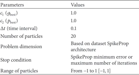
Table 1: PSO parameters used in SpikeProp.

Parameters Values

𝑐1(𝑔best) 1.0

𝑐2(𝑝best) 1.0

Δ𝑡(time interval) 0.1

Number of particles 20

Problem dimension Based on dataset SpikeProp

architecture

Stop condition SpikeProp minimum error or

maximum number of iterations

Range of particles From−1 to 1[−1, 1]

The number of particles in SpikeProp using PSO signifi-cantly affects the execution time. There is a tradeoff between the size of the practical swarms and the execution time. PSO with a well-selected parameter set can perform well under all

circumstances [30].

In this study, the parameters that have been used are

summarized inTable 1, while particle position (weight and

bias values) is initialized randomly with initial position velocity value set at 0.

Each particle position of the swarm is represented by a set of the weights for the current iteration. The dimension of the practical swarm determines the weight number of the network. In order to minimize the learning error, the particle should move within the weight space. Updating the weight of the network means changing the position in order to reduce the number of iterations. For each iteration, a new velocity calculation takes place to determine the new particle position movement. A set of new weights is used to obtain the new error, thus a new position. For PSO, the new weights are registered even if there is no noticeable improvement. This process applies for all particles. The global best particle position is the one with the least number of errors. The training process stops when the target minimum error is reached or the numbers of computational processes exceed the number of iterations allowable. When the training is complete, the weights are used to compute the classification error for the training patterns. The same patterns are used to test the network by using the same set of weights.

No researcher has yet used SpikeProp on PSO.𝑝bestvalue

and𝑔bestvalue are applied to solve problems associated with

the learning error. The SpikeProp weight and SpikeProp bias are achieved by adding the calculated velocity value

as shown in (1) and (2). A new set of positions is used to

produce the new learning error. In this proposed method, the classification dataset output has been written in a minimum number of iterations with the lowest error. The summary on

PSO-SpikeProp learning process is shown inFigure 1.

𝑤_𝑖𝑗new= 𝑤_𝑖𝑗old+ Δ𝑤_𝑖𝑗∗ Δ𝑡󵄨󵄨󵄨󵄨󵄨(𝑡)_𝑡=𝑡𝑑

𝑗, (1)

Δ𝑤𝑖𝑗(𝑛)=𝑐1∗ (𝑝best,𝑛− 𝑤𝑖𝑗(𝑛))+𝑐2∗(𝑔best,𝑛−𝑤𝑖𝑗(𝑛))󵄨󵄨󵄨󵄨_󵄨(𝑡)_𝑡=𝑡𝑑

𝑗.

(2)

Particles

Output

Particles

Remove vector

End of hidden

or output matrix

Yes No

Particles

input

position

Train SpikeProp using initial particle

with the current

initial weights over all

Calculate velocity and update all particles

Targeted learning error or

maximum number of

iterations No

Yes W

W

ReplaceWiby

i + 1

...

W

Wposition

. . .

hidden Hidden

W W

. . .

Initialize particleW

W i → 1

HiddenW OutputW

N

...

W N

i >size

w2 w1 w2

w1

W1

W2

W1

W2

gbest

Compare eachgbest

particles to obtainpbest

Comparegbestwith the

positions based ongbest

andpbestparticles

previous best to obtaingbest

Figure 1: PSO-SpikeProp learning process.

In this proposed technique, the PSO is applied to

SpikeP-rop algorithm (refer toFigure 1). Equation (1), the new weight

(5)

of𝑝best and𝑔best. In (2),Δ𝑤_𝑖𝑗(𝑛)subtracts the dimensional weight of the element from the dimension from the best vector and then multiplies this by a random number (between

0.0 and 1.0) and an acceleration constant (𝑐₁ and 𝑐₂). A

number of particles have been used to solve 8 different dataset problems. The objectives of the study are to reduce errors, enhance the learning rate of SpikeProp, and to speed up

the algorithm process. Figure 1shows that particle swarms

with initial random rates have different mean squared error (MSE). During the learning process, all particles move together to get𝑝bestand𝑔best.𝑔bestfit is an optimum solution.

3.2. Proposed 𝜇 Angle Driven Dependency Learning Rate

(Model 2). The proposed𝜇angle driven dependency learning

rate is an extension of Chan’s [31] adapted learning rate and

momentum during the training used in BP. This proposed method enhances SpikeProp learning according to the angle

calculation betweenΔ𝐸(𝑛)and Δ𝑤(𝑛 − 1). The adaptation

adjusts the angle at 90 degrees as per the Pythagoras formula method to get the square of the hypotenuse that equals to the sum of the squares of the other two sides. If the angle is less than 90 degrees, the learning rate is increased inversely, but if the angle is larger than 90 degrees, the learning rate is decreased. These mathematical methods have been applied to enhance SpikeProp, as shown next.

(1) The angle 𝜃 between the change of errors and the

change of the weights can be calculated by

cos𝜃 (𝑛) = Δ𝑊 (𝑛 − 1)

√Δ𝐸 (𝑛)2_{+ Δ𝑊 (𝑛 − 1)}2

󵄨󵄨󵄨󵄨 󵄨󵄨󵄨󵄨 󵄨󵄨󵄨󵄨 󵄨 (𝑡) 𝑡=𝑡𝑑 𝑗 . (3)

(2) The adaption learning rate cab be calculated by using the flowing formula:

𝜇 (𝑛) = 𝜇 (𝑛 − 1) ∗ (1 + 0.5 ∗cos𝜃 (𝑛)) . (4)

(3) Adaption of the momentum can be acquired as follows:

𝛼 (𝑛) = 𝛼 (0) ∗ _{‖Δ𝑊 (𝑛 − 1)‖}‖Δ𝐸 (𝑛)‖ 󵄨󵄨󵄨󵄨_{󵄨󵄨󵄨󵄨}(𝑡)

𝑡=𝑡𝑑

𝑗

. (5)

(4) As mentioned previously, the weights can be changed as follows:

Δ𝑊_𝑖𝑗(𝑛) = 𝜇 (𝑛) ∗ (_𝜕𝑊𝜕𝐸

𝑖𝑗) + 𝛼 (𝑛) ∗ Δ𝑊𝑖𝑗(𝑛 − 1)

󵄨󵄨󵄨󵄨 󵄨󵄨󵄨󵄨 󵄨󵄨 𝑡 𝑡=𝑡𝑑 𝑗 . (6)

Fortunately, the learning rate is adapted much faster when we are using the modified adaptation rule:

𝜇 (𝑛) = 𝜇 (𝑛 − 1) ∗ (1 + 0.1 ∗cos𝜃 (𝑛)) . (7)

Moreover, a backtracking strategy has been used, which reruns learning steps taking more than half learning rate time if total error increases. From this it can be concluded that the learning rate gets improved in Spikeprop with a higher rate than the standard SpikeProp.

3.3. Merging Model 1 with Model 2 for Enhancing SpikeProp

(Model 3). In order to get better performance and enhance

the operation of Spikeprop, a merging process between Model 1 and Model 2 (resulting in Model 3) has been carried out. Model 3 has an architecture which is partly PSO and partly angle driven dependency learning rate system. The flowchart

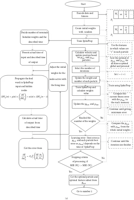
inFigure 2shows the general working of Model 3.

3.4. Error Measurement Functions. The target of the

Spike-Prop algorithm is to learn a set of target firing times, denoted

by{𝑡𝑑_𝑗}, at the output neurons𝑗 ∈ 𝐽for a given set of input

patterns{𝑃[𝑡_𝑗⋅ ⋅ ⋅ 𝑡_ℎ]}, where𝑃[𝑡_𝑗⋅ ⋅ ⋅ 𝑡_ℎ]defines a single input

pattern described by single spike times for each neuronℎ ∈

𝐻. Given the desired spike times{𝑡𝑎_𝑗}and actual firing times

{𝑡𝑎

𝑗}, this error function is defined by

(a) MSE= 1

𝑛 𝑛 ∑ 2−1

(𝑡𝑎

𝑗 2− 𝑡𝑑𝑗 2)

2

. (8)

This thesis uses other error functions such as RMSE (9),

MAPE (10) and MAD (11) to get more validation to evaluate

the accuracy of SpikeProp (SNN) that has been enhanced and proposed (Models 1, 2, and 3).

Consider

(b) RMSE= √1

𝑛 𝑛 ∑ 2−1

(𝑡𝑎

𝑗 2− 𝑡𝑑𝑗 2)

2

, (9)

(c) MAPE=

𝑛 ∑ 2−1 󵄨󵄨󵄨󵄨 󵄨󵄨󵄨󵄨 󵄨󵄨󵄨 𝑡𝑎

𝑗 2− 𝑡𝑑𝑗 2

𝑡𝑑 𝑗 2 󵄨󵄨󵄨󵄨 󵄨󵄨󵄨󵄨 󵄨󵄨󵄨∗ 100

𝑛 , (10)

(d) MAD=

𝑛 ∑ 2−1 󵄨󵄨󵄨󵄨

󵄨𝑡𝑗 2𝑎 − 𝑡𝑑𝑗 2󵄨󵄨󵄨󵄨󵄨

𝑛 . (11)

4. Results and Discussion

This section presents the results of study on learning of Spike-Prop network based on the proposed method of improved SpikeProp. The results for all datasets involved are analyzed based on the convergence to MSE, RMSE, MAPE, and MAD with their classification performance. The results of the proposed methods for each dataset are analyzed based on performance (accuracy). For analysis purposes, methods of improved SpikeProp are used to train and optimize the networks, comparing different measurements of error. The results of SpikeProp based on the proposed method of improved SpikeProp are presented in the following subsec-tions.

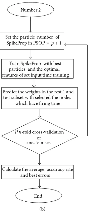
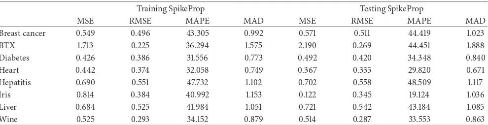
4.1. Results and Analysis of Standard SpikeProp. This section

presents the result of standard SpikeProp for all datasets. The results are analyzed based on the convergence to MSE, RMSE, MAPE and MAD findings with their classification

performance as shown inTable 2. All experiments for

stan-dard SpikeProp are based on ten runs. FromTable 2, RMSE

(6)

Go to number 2

0 or Start

Encode data and futures

Create initial weights with random

Train SpikeProp

Calculate velocity and update position based

particles

Select the number of iterations

Update the weight and number of each particle

Train SpikeProp and calculate weights

value

Learning error (best error as

time of SpikeProp

Get the optimal particle and optimal feature subset from

Reached the number of the weights

Stopping criteria

of processing if

Use the features in which values are “1” in each particle

Save the optimal of

all fitness optimal global and personal

Train using SpikeProp

Compare the current fitness error

the stack memory

whole initial weights Continue until getting

minimum error

Continue until the iteration size finishes Yes

Yes

No No Decide number of terminals

Initialize weights and the

described time

Present actual time of

input and described time

of output

Propagate the feed ward in SpikeProp input and hidden

nodes

Calculate actual time

of output from

described time

Get the error from

Adjust the initial

weights for the

nodes active with

the firing time

MSE(W_i) >MSE(W_j)

Seti = i + 1

1

m

m or 0 1

· · ·

𝜕E

𝜕wk

ij

𝜕E

𝜕ti

𝜕t_i

𝜕xi

ΔW_ij(n) = 𝜇(n) × 𝜕E

𝜕W_ij = 𝛼(n) × ΔWij(n − 1)

W1

P1

P₁

) (

= 𝛿_iyk

j

ong_best andp_best

Update thegbest

g_best

andpbest

g_bestand each particle best error aspbest) depends on the

g_bestandp_bestfor

with thepbest in

Compare thegbest

withpbest from the

(a)

(7)

Set the particle number of

Train SpikeProp with best particles and the optimal features of set input time training

Predict the weights in the rest 1 and test subset with selected the nodes

which have firing time

of

Calculate the average accuracy rate and best errors

Number 2

End mes>mses

SpikeProp in PSOP= p + 1

P n-fold cross-validation

(b)

Figure 2: Merge Model 1 with Model 2 learning process.

Heart, Iris, Diabetes, Breast Cancer, Liver, Hepatitis, and XOR, respectively. The RMSE is also better than MAPE, and MAD error measurements for all datasets. These show that the SpikeProp algorithm also demonstrates in a direct way that networks of spiking neurons can carry out complex, nonlinear tasks in a temporal code. As the experiments indicate, the SpikeProp algorithm is able to perform correct classification on nonlinearly separable datasets with all types of errors measurement compared to traditional sigmoidal

networks (BP) as shown in Table 3. Table 2 illustrates a

comparison of the measurements between the training and testing of SpikeProp algorithm. From this table, we can see that the SpikeProp converges with less errors than standard BP.

4.2. Results and Analysis of Standard BP. The analyses of

standard BP for all datasets are validated based on MSE,

RMSE, MAPE, and MAD as shown in Table 3. From the

training part inTable 3, the RMSE is better than MSE for

the training datasets of Diabetes, Heart, Breast Cancer, Liver, Hepatitis, Wine, Iris, BTX, and XOR, respectively. The MSE is also better than MAPE and MAD for all datasets except BTX, which shows that MAD values are less compared to MSE. This traditional BP network is widely used by other researchers for

classification problems. Bohte et al. [18] designed SpikeProp

for BP learning strategy; the comparisons between BP and

SpikeProp are given in Tables 2 and 3. It shows that BP

generates higher errors compared to SpikeProp.

4.3. Analysis of the Proposed Model 1: PSO-Spikeprop. Table 4

reveals the MSE generalization from the training part. MSE gives better results on Diabetes, Heart, Wine, and Breast Cancer datasets and least competitive for Liver, Hepatitis, Iris, BTX, and XOR datasets. For RMSE, the proposed PSO-SpikeProp is better for Wine, BTX, Diabetes, Iris, and Heart and less competitive in Liver, Breast Cancer, Hepatitis, and XOR, respectively. For MAD, the finding is better in Breast Cancer, Diabetes, and Heart and worse in Wine, Liver, Iris Hepatitis, BTX, and XOR, respectively. On the other hand, MAPE for PSO-SpikeProp gives higher error but still better than standard SpikeProp algorithm.

The PSO-SpikeProp gives the smallest error in MAPE compared to standard Spikeprop. However, PSO-SpikeProp stands out to be better if RMSE is being compared. Since the errors are squared before they are averaged, the RMSE gives a relatively low error rates, although the MSE has close

values to RMSE as shown in Table 4. Therefore, Model 1:

(8)

Table 2: Analysis for standard SpikeProp algorithm.

Training SpikeProp Testing SpikeProp

MSE RMSE MAPE MAD MSE RMSE MAPE MAD

Breast cancer 0.549 0.496 43.305 0.992 0.571 0.511 44.419 1.023

BTX 1.713 0.225 36.294 1.575 2.190 0.269 44.451 1.888

Diabetes 0.426 0.386 31.556 0.773 0.492 0.420 34.348 0.840

Heart 0.442 0.374 32.058 0.749 0.367 0.335 29.820 0.671

Hepatitis 0.690 0.551 47.732 1.102 0.702 0.558 48.509 1.117

Iris 0.814 0.384 40.992 1.153 0.122 0.345 19.124 1.036

Liver 0.684 0.525 41.984 1.051 0.721 0.542 43.184 1.085

Wine 0.525 0.293 34.152 0.879 0.514 0.287 33.553 0.863

Table 3: Analysis for standard BP algorithm.

Training BP Testing BP

Breast cancer 0.672 0.525 54.759 1.278 0.816 0.638 54.443 1.277

BTX 1.982 0.796 88.018 2.575 2.707 0.798 88.344 2.588

Diabetes 0.510 0.429 37.576 1.271 0.792 0.627 59.208 1.255

Heart 0.608 0.477 41.902 1.270 0.805 0.633 55.724 1.267

Hepatitis 0.837 0.646 55.588 1.293 0.837 0.647 55.607 1.294

Iris 0.874 0.763 69.176 2.290 0.865 0.759 68.660 2.278

Liver 0.826 0.641 56.315 1.283 0.831 0.643 56.459 1.287

Wine 0.749 0.419 72.471 1.119 0.753 0.408 72.649 1.125

Table 4: Analysis for Model 1.

Training Model 1 Testing Model 1

Breast cancer 0.356 0.361 35.261 0.723 0.367 0.372 36.268 0.745

BTX 1.270 0.199 35.596 1.398 1.763 0.247 43.785 1.730

Diabetes 0.241 0.245 22.650 0.490 0.284 0.277 25.778 0.555

Heart 0.2828 0.281 26.813 0.563 0.272 0.272 25.997 0.545

Hepatitis 0.483 0.448 42.640 0.896 0.494 0.457 43.609 0.915

Iris 0.351 0.251 33.270 0.754 0.112 0.147 18.38 0.443

Liver 0.360 0.340 31.854 0.680 0.383 0.357 33.332 0.714

Wine 0.312 0.196 25.033 0.590 0.305 0.196 25.269 0.589

the smallest error during the implementation. For this model we conclude that error can be reduced to reach the minimum value.

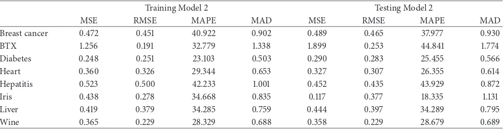
4.4. Analysis of the Proposed Model 2: SpikeProp with Angle

Driven Dependency (𝜇). Similar to previous experiments, the

results of Model 2 of SpikeProp with angle driven dependency are computed based on MSE, RMSE, MAPE, and MAD

error measurements.Table 5shows the findings of the model,

which are based on ten independent runs on both training and testing datasets, respectively. The average testing errors are being calculated along with the standard deviations for all datasets.

As can be seen fromTable 5, it is interesting to see the

small standard deviations for all error rates on the training set

and the testing set in all datasets. The results of this proposed Model 2 have demonstrated that the generalization of MSE is better for Diabetes, Heart, and Wine datasets, while the results for Liver, BTX, Hepatitis, Iris, Breast Cancer, and XOR datasets are the least competitive. The results also have shown that the RMSE is better on all datasets and less competitive for other error measurements except for the Diabetes dataset which has better MSE values compared to RMSE. In general, the diversity of errors rates (MSE, RMSE, MAPE, and MAD) for this proposed Model 2 is considered better for all datasets. According to this model, we can find that the error is less than BP and SpikeProp standard.

4.5. Analysis of the Proposed Model 3: Hybridization of Model

(9)

Breast cancer 0.472 0.451 40.922 0.902 0.489 0.465 37.977 0.930

BTX 1.256 0.191 32.779 1.338 1.899 0.253 44.841 1.774

Diabetes 0.248 0.251 23.103 0.503 0.290 0.283 25.455 0.566

Heart 0.360 0.326 29.344 0.653 0.327 0.307 26.355 0.614

Hepatitis 0.523 0.500 42.233 1.001 0.452 0.435 43.929 0.872

Iris 0.438 0.278 34.668 0.835 0.117 0.377 18.335 1.131

Liver 0.419 0.379 34.285 0.759 0.444 0.397 34.289 0.795

Wine 0.365 0.229 28.329 0.688 0.358 0.229 28.679 0.689

Breast cancer 0.350 0.355 34.812 0.711 0.361 0.367 35.863 0.734

BTX 0.972 0.162 27.401 1.138 1.592 0.226 39.155 1.585

Diabetes 0.211 0.212 20.218 0.425 0.251 0.245 23.496 0.491

Heart 0.252 0.250 24.543 0.501 0.241 0.240 23.634 0.481

Hepatitis 0.437 0.421 41.179 0.843 0.446 0.431 42.194 0.863

Iris 0.330 0.244 32.747 0.732 0.105 0.153 17.576 0.461

Liver 0.359 0.339 31.778 0.678 0.380 0.356 33.296 0.712

Wine 0.263 0.168 22.186 0.506 0.273 0.178 23.637 0.535

two good genes, it may be possible to get good SpikeProp algorithm by merging (hybridizing) two good techniques. Therefore, this paper is concerned about the merging imple-mentation of Model 1 and Model 2 (to get Model 3) as

maintained inFigure 2.

In this section, we hybridize Model 1: PSO-SpikeProp and Model 2: SpikeProp with angle driven dependency to obtain a better performance for error rates (MSE, RMSE, MAPE, and MAD). We notice that the performance mea-surement is better than in the previous proposed method

when the hybridization takes place as shown in Table 6.

The experiments are based on 10 independent runs for the training and testing for all datasets, respectively. The results have revealed that generalization of error rates in RMSE is better for BTX, Wine, Diabetes, Iris, and Heart datasets and the least competitive for Breast Cancer, Hepatitis, Liver, and XOR datasets. Similarly, the result of MSE error rate has been demonstrated to be less better for Diabetes, Heart, Wine, Iris, Breast Cancer, Liver, Hepatitis, and BTX datasets, respectively. To get better performance, we hybridized Model 1 and Model 2, to get Model 3, to minimize the error to reach the optimum error value.

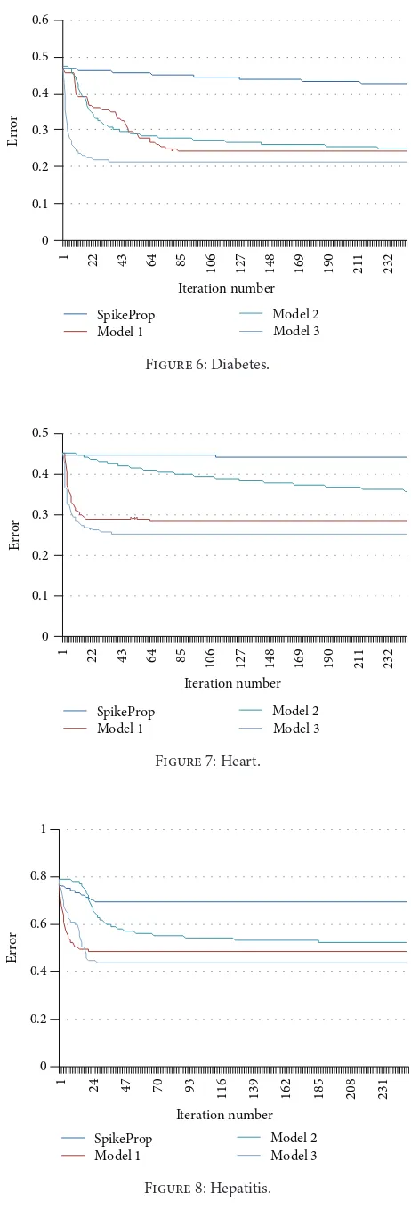
4.6. Analysis and Result for Proposed Methods Based on Error.

In this section, the spiking neural network and SpikeProp use the encoding by depending on the timing of spike, where the first spike has a higher weight than the last one. Since a biological neuron uses few milliseconds to process information data, only few spikes are required and emitted, however the few first spikes with highest value information

can contribute to all process learning, as we used Gaussian

function for encoding. Figures3–10show the convergence

of the error and the number of iterations of the Spikeprop standard and the proposed methods for the improved SpikeP-rop in the classification Liver dataset, Breast Cancer, BTX, Diabetes, Heart, Hepatitis, Iris, and Wine data problems. The SpikeProp standard configuration had a much slower rate of convergence, as can be clearly seen in the plot. Although its rate of progress gradually slow down from the beginning till last iteration but kept in high error in the MSE, despite this

slowdown in all data problems as shown in Figures3–10.

4.6.1. Analysis Error and Iterations of Model 1

(PSO-SpikeP-rop). We also see from the convergence that the proposed

method for improved SpikeProp is much better than standard SpikeProp as PSO-SpikeProp (Model 1) had dramatic slow-down from the first 10 iterations slow-down to iteration number 40, and afterwards the plot got a slight slowdown in Liver as

shown inFigure 3. In Breast Cancer data problem inFigure 4

the curve steps down at the start in error near to 0.5 until 0.38 exactly and then it continued descending to the last itera-tion at error 0.35 gradually. PSO-SpikeProp (model 1) is the first model from the proposed methods; the error turned down quickly in the first 10 iterations at 1.78 and continued to drop down till the last iteration in the error 1.27 in the

BTX data problem as seen inFigure 5. Also in Diabetes data

problem inFigure 6 the curve for the error steps down so

(10)

Er

ro

r

Iteration number 0

0.2 0.4 0.6 0.8 1

1 ₁₉ ₃₇ ₅₅ ₇₃ ₉₁

10

9

12

7

14

5

16

3

18

1

19

9

21

7

23

5

SpikeProp Model 1

Model 2 Model 3

Figure 3: Liver.

Er

ro

r

Iteration number 0

0.1 0.2 0.3 0.4 0.5 0.6 0.7

1 ₂₂ ₄₃ ₆₄ ₈₅

106 127 148 169 190 211 232

SpikeProp Model 1

Model 2 Model 3

Figure 4: Breast cancer.

0 0.5 1 1.5 2 2.5

1 ₂₁ ₄₁ ₆₁ ₈₁

101 121 141 161 181 201 221 241

SpikeProp Model 1

Model 2 Model 3

Er

ro

r

Iteration number

Figure 5: BTX.

Er

ro

r

Iteration number 0

0.1 0.2 0.3 0.4 0.5 0.6

1 ₂₂ ₄₃ ₆₄ ₈₅

106 127 148 169 190 211 232

SpikeProp Model 1

Model 2 Model 3

Figure 6: Diabetes.

Er

ro

r

Iteration number 0

0.1 0.2 0.3 0.4 0.5

1 ₂₂ ₄₃ ₆₄ ₈₅

106 127 148 169 190 211 232

SpikeProp Model 1

Model 2 Model 3

Figure 7: Heart.

Er

ro

r

Iteration number 0

0.2 0.4 0.6 0.8 1

1 ₂₄ ₄₇ ₇₀ ₉₃

116 139 162 185 208 231

SpikeProp Model 1

Model 2 Model 3

(11)

0 0.2 0.4 0.6 0.8 1 1.2

1 ₂₄ ₄₇ ₇₀ ₉₃

116 139 162 185 208 231

SpikeProp

Iteration number

Model 1

Model 2 Model 3

Er

ro

r

Figure 9: Iris.

0 0.1 0.2 0.3 0.4 0.5 0.6

1 ₂₄ ₄₇ ₇₀ ₉₃

116 139 162 185 208 231

Iteration number

SpikeProp Model 1

Model 2 Model 3

Er

ro

r

Figure 10: Wine.

it was a little sloped and stopped at the last iteration in error 0.24.

As we can see fromFigure 7in Heart problem the curve

in error has dropped in a dramatic manner in the first 15 iterations in error from 0.45 to 0.28, and then the dropping is slowed down till iteration number 67 in error 0.28 and continued steadily till the last iteration for the same error. From the same proposed model in Hepatitis data problem

inFigure 8 we can see that the slope of the curve starts at

the first 15 iterations in a fast way in error 0.76 to 0.49, and then it slows down till iteration number 38 in error 0.48 and it stays likely stable till the last iteration. In Iris data problem

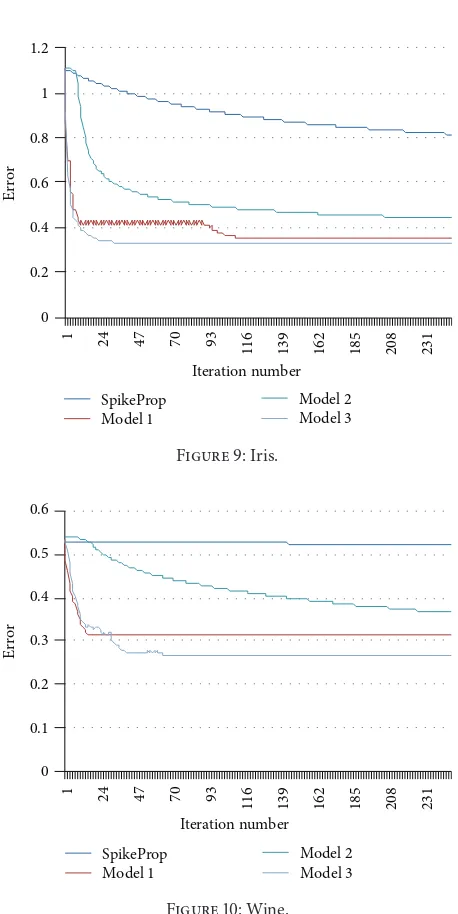
in this model the plot fromFigure 9is stepped down in very

fast drop from the first 10 iterations in error 1.105, and then it is zigzagged in error range 0.433 to 0.410 till iteration number 90 and then immediately fell down till the iteration number 112 in error 0.351 and it stayed on it till last iteration. Finally the plot of the error is stepped down in a high manner in the first

15 iterations of error 0.534 to 0.312, and then it stabilized in this error till the last iteration in Wine data problem as shown

inFigure 10. From this model we have seen from Figures3–10

how to obtain the list error from list iteration number from the whole data sets.

4.6.2. Analysis Error and Iterations of Model 2. In the second

improvement for SpikeProp through the learning rate angle driven dependency (Model 2), we can also notice in Liver data

problem as shown inFigure 3that it has a slight dropping for

the first 10 iterations in error around 0.75 and got a huge fall down till iteration number 50 for the error of nearly 0.55 and then it had a slight dropping till last iteration for the error

0.4. In the same model in Breast Cancer problem inFigure 4,

the plot started to fall down on the first 20 iterations in error 0.57 until 0.47 gradually. Also the curve in BTX data problem

as shown inFigure 5 start dropping down from the first 5

iterations in error 1.73 to 1.72, and it is fluctuated between the 6th iteration and iteration number 197 of the error range 1.73 to 1.31. Afterwards it has a steady drop till iteration 250 at error interval 1.30 to 1.25. From the result in Diabetes problem at

the same Model 2 on the plot inFigure 6, the error in first

seven iterations has dropped down slowly at error 0.47; after that it stepped down quickly till iteration number 20 in error 0.35 and then continued steadily until the last iteration for

error 0.24. In the Heart data problem fromFigure 7, the plot

is stepped down from first iteration in error 0.45 until last iteration in error 0.36, and in some iterations, it is stable and then it continues descending. Also in Hepatitis data problem as shown inFigure 8, it has a stable error of 0.786 for the first 5 iterations, and then it start to fall down till iteration number 80 for error 0.549; after that it has a slower dropping till last iteration on error 0.523 in a sequence stepping down.

FromFigure 9as we can see clearly the curve is dropped

down slowly in first 10 iterations in error 1.111 till 1.040; then it accelerates in dropping till iteration number 55 of error 0.53 and the drop slows down till last iteration in 0.438 error

in the Iris data problem. Finally from Figure 10 in Wine

data problem the plot shows Model 2 (learning rate angle driven dependency) is almost steady in first 15 iterations in error 0.538 to 0.526, and then the dropping got accelerated continuously till last iteration for error 0.366.

4.6.3. Analysis Error and Iterations of Model 3 (SpikeProp with

Angle Driven Dependency (𝜇)). (PSOSpikeProp and

Learn-ing Rate Angle Driven Dependency) or (model 3), in Liver

dataset as it is clear from Figure 3the plot it provides the

best enhancement result for the convergence of error and number of iteration. The slant starts from the first iteration in the error a bit less than 0.8 till iteration number 20 impressively, and then a gradual descending has been done till last iteration of error close to 0.354. The curve from

Figure 5witnessed a dramatic drop in first 10 iterations

start-ing from error 1.95 and the drop decreases till last iteration

at error 0.97. We can notice from the curves inFigure 4that

(12)

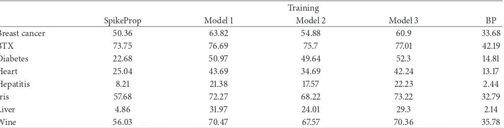
Table 7: Result of training in terms of accuracy.

Training

SpikeProp Model 1 Model 2 Model 3 BP

Breast cancer 50.36 63.82 54.88 60.9 33.68

BTX 73.75 76.69 75.7 77.01 42.19

Diabetes 22.68 50.97 49.64 52.3 14.81

Heart 25.04 43.69 34.69 42.24 13.17

Hepatitis 8.21 21.38 17.57 22.23 2.44

Iris 57.68 72.27 68.22 73.22 32.79

Liver 4.86 31.97 24.01 29.3 2.14

Wine 56.03 70.47 67.57 70.36 35.78

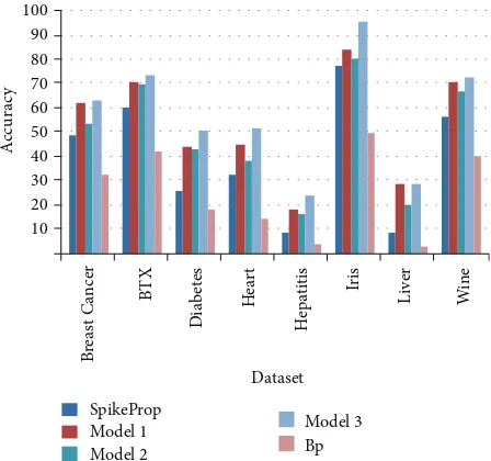
Table 8: Result of testing in terms of accuracy.

Testing

SpikeProp Model 1 Model 2 Model 5 BP

Breast cancer 48.82 62.7 53.46 63.28 32.21

BTX 60.52 71.15 70.42 73.57 41.77

Diabetes 25.99 44.45 43.31 50.8 18

Heart 32.81 45.4 38.56 51.81 14.64

Hepatitis 8.78 18.42 16.5 23.65 4.33

Iris 77.66 84.66 80.73 96.03 50.03

Liver 8.55 28.55 20.48 28.79 2.8

Wine 56.84 70.53 67.53 73.24 40.13

the first iteration of error 1.93 to last iteration of error 0.97. From this we can see that most impact on SpikeProp standard is from PSO-SpikeProp and the leaning rate methods, and other proposed methods have less impact on BTX data

problem as shown inFigure 5.

From the plot in Figure 6, this model started to drop

down in a very fast way in first 10 iterations for error 0.7 to error 0.24, and then it started to slow down till iteration number 43 in error 0.21, and then it became almost stopped in error 0.21 till last iteration; we conclude from the comparison of the previous result that the model 3 gives the best and the least error from all other methods in Diabetes dataset. We can see from the plot that the curve fell down quickly in first 10 iterations for error range 0.45 to 0.29, and then the dropping started to slow down till iteration number 30 in error 0.258, then it got almost steady till last iteration in error 0.252. From the previous it is obvious that this model is the best among all

the other models for Heart data problem as seen inFigure 7.

This merge (Model 3) starts to drop down quickly from the first iteration for the error 0.787 until iteration number 30 for error 0.438, and then it stays stable until last iteration, as it

is obvious fromFigure 8and the results that the third model

has the most impact on SpikeProp compared to the previous

models for Hepatitis data problem. Finally fromFigure 9it

can be seen that the plot in this merge model started to step down quickly in first 30 iterations in error 1.107 to 0.332 and then it got steady for the same error till last iteration. This can show that the third model of improving SpikeProp gives the best result compared to other previous methods in Iris data problem.

Lastly, Model 3 is merging between Model 1 and Model 2 (PSO-SpikeProp and learning rate angle driven depen-dency); this merging model has a high impact on enhancing

SpikeProp as it is seen in the curve ofFigure 10that in Wine

data problem the slope is dropped quickly starting from first iteration of error 0.533 till iteration number 70 of error 0.263 and then it becomes almost stable till last iteration.

4.7. Result and Analysis Comparison of the Proposed

Meth-ods in Terms of Accuracy. This section displays the result

of SpikeProp standard besides the proposed methods for enhanced SpikeProp measured in terms of accuracy. The experiments are run 10 s, 10 dependent runs on training

and testing for all datasets, respectively (refer to Tables 7

and8 and Figures11 and12). As it is shown inTable 7 for

training, the first proposed method PSO-SpikeProp (Model 1) is evaluated in terms of accuracy; we can see that we got the value in Breast Cancer better than SpikeProp standard and proposed methods except Model 5. Regarding the BTX dataset problem, it is also better than SpikeProp standard and other proposed methods except Model 3. The generalization of accuracy for the proposed method PSOSpikeProp is better than SpikeProp standard and learning rate angle driven dependency (Model 2) in all datasets. Learning rate angle driven dependency is our proposed method; it is better than SpikeProp standard in all datasets. Finally, Model 3 is merging model (PSO-SpikeProp and Learning Rate Angle Driven

Dependency) as illustrated inFigure 11andTable 7that it is

(13)

0 20 40 60 80 100 SpikeProp Model 1 Model 2 Model 3 Dataset Bp B re ast C ancer BT X Dia b et es He ar t H epa ti ti s Ir is Li ve r Wi n e A cc urac y

Figure 11: Results in training of the proposed methods in terms of accuracy. 10 20 30 40 50 60 70 80 90 100 SpikeProp Model 1 Model 2 Model 3 Dataset Bp B re ast C ancer A cc urac y BT X Dia b et es He ar t H epa ti ti s Ir is Li ve r Wi n e

Figure 12: Results in testing of the proposed methods in terms of accuracy.

5. Conclusions

We introduced several extensions to the SpikeProp learn-ing algorithm that make it possible to learn not only the weights, but also the delays and synaptic time constants of the connections and the thresholds of the neurons. Due to these enhancements, smaller network architecture can be used. This is mainly due to the fact that delays can now be trained and need not be enumerated. The simple 8 data sets could be solved with the same precision as the original SpikeProp algorithm, less errors (making the simulation and learning phase of the network much faster), and an increased learning convergence. There are several proposed models needed to improve the performance of SpikeProp further; hybridization of two or more good architectures is carried

out (for instance the hybridization of Model 1 and Model 2 to obtain Model 3). The purpose of hybridization is to leverage the best function from each component of the hybrid. As an example, Model 3 is the hybridization of Model 1 which is PSO-SpikeProp (enhancement Spikeprop architecture by PSO) with Model 2 which is SpikeProp enhancement using angle driven dependency learning rate. For Model 3, when the position of search is far from the optimum, PSO is used to directly move the point of search close to the optimum. When the search point is close to the optimum, Model 3 switches over to the system where there is SpikeProp enhancement using angle driven dependency learning rate to reach the optimum position. Also a thorough analysis of the weight initialization problem is required. The convergence rate seems to be pretty sensitive to this. Several techniques used in classic neural networks to speed up backpropagation learning could be added to SpikeProp to further speed up learning.

References

[1] Y. J. Jin, B. X. Shen, R. F. Ren, L. Yang, J. Sui, and J. G. Zhao, “Prediction of the styrene butadiene rubber performance by emulsion polymerization using backpropagation neural

net-work,”Journal of Engineering, vol. 2013, Article ID 515704, 6

pages, 2013.

[2] W. Gerstner, R. Kempter, J. L. van Hemmen, and H. Wagner,

Hebbian Learning of Pulse Timing in the Barn Owl Auditory System in Maass, 1999.

[3] A. Belatreche and R. Paul, “Dynamic cluster formation using

populations of spiking neurons,” in Proceedings of the 2012

International Joint Conference on Neural Networks (IJCNN ’12), pp. 1–6, June 2012.

[4] D. Ferster and N. Spruston, “Cracking the neuronal code,”

Sci-ence, vol. 270, no. 5237, pp. 756–757, 1995.

[5] S. Thorpe, A. Delorme, and R. van Rullen, “Spike-based

strate-gies for rapid processing,”Neural Networks, vol. 14, no. 6-7, pp.

715–725, 2001.

[6] N. Kasabov, “Evolving, probabilistic spiking neural networks and neurogenetic systems for spatio- and spectro-temporal data

modelling and pattern recognition,” inProceedings of the IEEE

World Congress on Computational Intelligence (WCCI ’12), vol.

7311 ofLecture Notes in Computer Science, pp. 234–260, 2012.

[7] C. M. Bishop,Neural Networks for Pattern Recognition, 2000.

[8] S. Haykin, Neural Networks: A Comprehensive Foundation,

Prentice Hall PTR, 1998.

[9] M. Negnevitsky,Artificial Intelligence: A Guide to Intelligent

Sys-tems, Addison Wesley, 2002.

[10] N. Kasabov, “Integrative connectionist learning systems in-spired by nature: current models, future trends and challenges,”

Natural Computing, vol. 8, no. 2, pp. 199–218, 2009.

[11] Gewaltig,Evolution of Synchronous Spike Volleys in Cortical

Net-works: Network Simulations and Continuous Probabilistic

Mod-els, vol. 1822 ofLecture Notes in Artificial Intelligence, Springer,

2000.

[12] S. Thorpe and J. Gaustrais, “Rank order coding,” in

Compu-tational Neuroscience: Trends in Research, pp. 113–118, Plenum Press, New York, NY, USA, 1998.

[13] N. Kasabov, “To spike or not to spike: probabilistic spiking

(14)

[14] W. Maass, “Computing with spiking neurons,” inPulsed Neural Networks, W. Maass and C. Bishop, Eds., vol. 2, pp. 55–85, MIT Press, Cambridge, Mass, USA, 2001.

[15] D. Mishra, A. Yadav, A. Dwivedi, and P. K. Kalra, “A neural network using single multiplicative spiking neuron for function

approximation and classification,” inProceedings of the

Inter-national Joint Conference on Neural Networks (IJCNN ’06), pp. 396–403, July 2006.

[16] A. Gr¨uning and I. Sporea, “Supervised learning of logical operations in layered spiking neural networks with spike train

encoding,”Neural Processing Letters, vol. 36, no. 2, pp. 117–134,

2012.

[17] W. Gerstner and W. M. Kistler,Spiking Neuron Models,

Cam-bridge University Press, 2002.

[18] S. M. Bohte, J. N. Kok, and H. La Poutr´e, “Error-backprop-agation in temporally encoded networks of spiking neurons,”

Neurocomputing, vol. 48, no. 1–4, pp. 17–37, 2002.

[19] J. ˇSıma, “Gradient learning in networks of smoothly spiking neurons,” Tech. Rep. 1045, 2009.

[20] D. E. Rumelhart, G. E. Hinton, and R. J. Williams, “Learning

representations by back-propagating errors,”Nature, vol. 323,

no. 6088, pp. 533–536, 1986.

[21] W. Gerstner and W. M. Kistler, Spiking Neuron Models: An

Introduction, Cambridge University Press, 2002.

[22] S. C. Moore,Back-propagation in spiking neural networks [M.S.

thesis], Department of Computer Science, University of Bath, Bath, UK, 2002.

[23] J. Xin and M. J. Embrechts, “Supervised learning with spiking

neural networks,” in Proceedings of the International Joint

Conference on Neural Networks (IJCNN ’01), pp. 1772–1777, July 2001.

[24] B. Schrauwen and J. V. Campenhout, “Parallel hardware imple-mentation of a broad class of spiking neurons using serial

arithmetic,” inProceedings of the 14th European Symposium on

Artificial Neural Networks, M. Verleysen, Ed., pp. 623–628, 2007.

[25] K. Berkovec, Learning in networks of spiking neurons [M.S.

thesis], Faculty of Mathematics and Physics, Charles University, Prague, Czech Republic, 2006.

[26] P. Tiˇno and A. J. S. Mills, “Learning beyond finite memory in

recurrent networks of spiking neurons,”Neural Computation,

vol. 18, no. 3, pp. 591–613, 2006.

[27] I. R. Fiete and H. S. Seung, “Gradient learning in spiking neural

networks by dynamic perturbation of conductances,”Physical

Review Letters, vol. 97, no. 4, Article ID 048104, 2006.

[28] K. Mergenthaler and R. Engbert, “Modeling the control of

fixa-tional eye movements with neurophysiological delays,”Physical

Review Letters, vol. 98, no. 13, Article ID 138104, 2007. [29] K. Nakazawa, M. C. Quirk, R. A. Chitwood et al., “Requirement

for hippocampal CA3 NMDA receptors in associative memory

recall,”Science, vol. 297, no. 5579, pp. 211–218, 2002.

[30] Y. Shi, Particle Swarm Optimization, IEEE neural Network

Society, 2004.

[31] L. W. Chan and F. Fallside, “An adaptive training algorithm for

back propagation networks,”Computer Speech and Language,

(15)

Submit your manuscripts at

http://www.hindawi.com

Operations

Research

Advances in

Hindawi Publishing Corporation

http://www.hindawi.com Volume 2013

Mathematical Problems in Engineering

Abstract and

Applied Analysis

ISRN

Applied Mathematics

http://www.hindawi.com Volume 2013 International Journal of

Combinatorics

Journal of Function Spaces and Applications

International Journal of Mathematics and Mathematical Sciences

Hindawi Publishing Corporation http://www.hindawi.com Volume 2013

ISRN

Geometry Hindawi Publishing Corporation

http://www.hindawi.com Volume 2013 Hindawi Publishing Corporation

Discrete Dynamics in Nature and Society

Advances in

Mathematical Physics

ISRN

Algebra

Probability

and

Statistics

Journal of

ISRN

Mathematical Analysis Hindawi Publishing Corporation

Journal of

Applied Mathematics

Sciences

Stochastic Analysis

International Journal of Hindawi Publishing Corporation

http://www.hindawi.com Volume 2013 Hindawi Publishing Corporation

The Scientific

World Journal

http://www.hindawi.com Volume 2013 ISRN

Discrete Mathematics

Hindawi Publishing Corporation http://www.hindawi.com

Differential

Equations

International Journal of

Volume 2013