Online Full Text

(1)

Abstract—This research aims to solve the supplier selection problem for the components of Hard Disk Drive using meta-heuristics. This problem is constrained by the limited budget and the requirement on the suppliers rating for the components. The problem’s objective is to maximize the total yield. This problem is considered as a NP-Hard problem with the formulation of a nonlinear integer programming problem. Four heuristics, which are Ant Colony Optimization (ACO), Improved Ant Colony Optimization (IACO), Genetic Algorithm (GA) and Tabu Search (TS), are proposed to solve this problem. IACO embeds the Neighborhood search and re-initialization technique. Using the data obtained from undisclosed HDD manufacturer, computational experiments are conducted under various budget constraints. The results from the experiments show that IACO can solve the problem with better efficiency compared with other methods under reasonable time.

Index Terms—Nonlinear Integer Programming, Heuristic, Yield Optimization, Supplier Rating, Hard Disk Drive.

I. INTRODUCTION

A hard disk drive (HDD) is a non-volatile storage device which stores digitally encoded data on rapidly rotating platters with magnetic surfaces. HDDs have been used in digital video recorders, digital audio players, personal digital assistants, digital cameras and video game consoles. Therefore, HDD manufacturers make high portable with high capacity HDD for various electrical and electronic devices, so it is critical to be able to support high variance of customer requirements such as capacity, size, technology and cost. Thus, the business owner needs to adjust or manage the strategies in term of manufacturing process to be more flexible in order to support the new product model in time. In today competitive market, minimizing HDD production cost and maximizing production yield are very critical. In this paper, the focus is on the product yield and the material because the product yield is highly affected by the yield of raw materials.

Manuscript received on June 28, 2010. This work was supported by Thailand Research Fund (TRF), National Research Council of Thailand (NRCT), Commission on Higher Education of Thailand, Faculty of Thammasat University and Thammasat University, Thailand.

*Wuthichai Wongthatsanekorn is a lecturer, Industrial Engineering Department, Faculty of Engineering, Thammasat University, Rangsit campus, Klongluang, Pathum-thani, 12120, Thailand (corresponding author; e-mail: [email protected])

N.Matheekrieangkrai is a Graduate Student in Industrial Engineering Department, Faculty of Engineering, Thammasat University, Rangsit campus, Klongluang, Pathum-thani, 12120, Thailand. (e-mail:[email protected])

Hence, an economical strategy is required to identify the optimal configuration of the components. This research work only considers the raw materials or material factor in 4M theory (man, machine, material and method) before they are loaded and preceded into the mass production. The engineers can emphasize on improving men, machines and methods instead. Each supplier offers different quality for its own component and the component yield for each supplier can be collected during prototype or pilot run.

The goal of this problem is to determine the best selection of materials from multiple suppliers for all HDD’s components so that the total product’s yield is maximized judging from the raw material defective rates. There are two main constraints in this problem. The first constraint is that there’s a limited budget that can be spent on selecting components from each supplier. Sometime choosing the best quality component might not be affordable. The second constraint deals with supplier’s rating. Hence, this problem is called HDD component yield optimization under budget and supplier’s rating constraints (YOBS). This problem is based on a series system with multiple-choice constraints incorporated at each subsystem. The problem can be formulated as a nonlinear binary integer programming problem and characterized as an NP-hard problem.

In the past decade, many heuristics have been proposed and successfully applied to the combinatorial optimization problem such as the traveling salesman problem (TSP), the quadratic assignment problem, the vehicle routing problem, and the job-shop scheduling problem. In this research, four heuristics are proposed to solve the YOBS problem. They are Ant Colony Optimization (ACO), Improved Ant Colony Optimization (IACO), Genetic Algorithm (GA) and Tabu Search (TS). In particular, the focus is on improving ACO by embedding neighborhood search and re-initialization technique. The numerical examples are performed based on the actual data of selected HDD module from undisclosed HDD manufacturer. The optimized result is shown in terms of solution quality and computational efficiency.

The organization of this paper is as follows: In Section 2, the problem formulation is introduced and expressed as nonlinear binary integer programming problem. The details of ACO, IACO, GA and TS are shown in Section III, IV, V and VI respectively. In Section VII computer simulation results are presented and numerical examples demonstrates the effectiveness of the algorithm. Finally, the conclusions are drawn in Section VIII.

Heuristics for Hard Disk Drive Component’s

Yield Optimization Problem under Budget and

Supplier’s Rating Constraints

(2)

II.PROBLEM FORMULATION

YOBS problem can be formulated by using indices, parameters and decision variables as follows.

Indices:

i : Index of components ,

i

=

1,..,

n

j : Index of suppliers ,

j

=

1,..,

ns

_i

l : Index of main components ,

l

∈

{1,.., }

n

Parameters:

n : Number of components i

ns

: Number of suppliers available for component i

ij

C : Unit Cost of component i from supplier j

ij

Y : Yield of the component i from supplier j ij

SR : Supplier’s rating of component i from supplier j minR: Minimum supplier rating

minS: Minimum average supplier rating B : Total available budget

Decision Variables:

1 if the component is supplied by supplier

0 otherwise

ij

i j

x = ⎨⎧

⎩

for i=1,2,...,n and j=1, 2,...,m_i

With these notations, the YOBS problem can be formulated as the following nonlinear binary integer (NBIP) programming problem:

(YOBS) Maximize

1 1 i ns n ij ij j i

Z

Y x

= =

⎛

⎞

=

_⎜

_⎟

⎝

∑

⎠

∏

(1)

Subject to 1 1 i ns n ij ij i j

C x

B

= =

≤

∑∑

(2)

1

k ns lj lj j

SR x

minR

l

=

≥

∀

∑

(3)

1 1 i ns n ij ij i j

SR x

minS

n

= =

⎛

⎞

⎜

⎟

⎝

∑∑

_{⎠ ≥}

(4) 1

1

i ns ij j

x

i

=

∀

∑

(5)

{ }

0,1

,

ij

x

=

∀

i j

(6) In this formulation, there are n components in selected HDD module. Each component ican be purchased from

i

ns different suppliers with different costs, qualities, yield, weights and other characteristics. The problem description is how to select the best set of suppliers to maximize product yield given limited allowable budget such that there is only one supplier chosen for each component.

The objective function represents the total yield from selected component. Note that this objective function is nonlinear because it’s a product of each component’s yield as shown in Constraint (1). Constraint (2) guarantees that the

limited budget will not be exceeded. Constraint (3) enforces that the main components must pass minimum rating from the selected supplier. Constraint (4) requires that the average supplier rating of all selected components is higher than the minimum requirement. Constraint (5) limits that only each component can be supplied by only one supplier. Last, constraint (6) define decision variable x_ij as the binary variable.

Table1: Assessment Criteria for supplier’s rating [1]

RATING >= 90 OUTSTANDING A

70=< RATING < 90 ACCEPTABLE B

50=< RATING < 70 NEEDS IMPROVEMENT C

RATING < 50 UNACCEPTABLE F

The example of assessment criteria for supplier’s rating is shown in Table 1. Normally, only suppliers with outstanding and acceptable (or level A and B) are considered. In the case study of Section VII, minR and minS values are set to 90.

Since the number of suppliers in HDD industry is large and one HDD model contains a lot of components, this combinatorial optimization problem contains exponential number of solutions. Solving this NBIP problem to obtain optimal solution using commercial software can be very time consuming. Therefore, four heuristics are proposed to solve the problem in order to find an efficient solution under reasonable computation time effort.

III. ANT COLONY OPTIMIZATION (ACO)

For ACO, each ant represents the solution or the combination of selected supplier for each component. These following ACO procedures are applied from [2, 3]. First, m ants or solutions are constructed based on state transition rule. Next, the amount of pheromone is updated by following global updating rule. The solutions are guided by both heuristic information and pheromone information to yield the best solution. These steps are then repeated many times based on the setting of cycle counter.

State transition rule

The state transition rule is applied for each ant and represented by p t_ijk( ). The probability that ant k selects component i from supplier j is shown in Eq. (7) below:

[ ] [ ]

[

] [

]

∑

= = i M m im im ij ij k ij t t t t t p 1 ) ( ) ( ) ( ) ( ) ( β α β α η τ η τ (7)

where τij is the pheromone intensity and ηij is the heuristic

information between component i and supplier j, respectively. In addition, α is the relative importance of the trail and β is the relative importance of the heuristic information. In this heuristic, the problem specific heuristic information can be obtained by using Eq. (8) below:

ij ij

ij Y

C

(3)

where Cij and Yij represent the associated cost and yield of

component i from supplier j respectively. Therefore, the supplier of component with smaller cost and higher yield has higher chance to be selected.

Global updating rule

During the constructing feasible solutions, it may be possible that an ant will result in an infeasible solution which violates the budget constraint or Eq. (2). To resolve this problem, high amount of pheromone is deposited if the constructed solution is feasible. On the other hand, low amount of pheromone is deposited if the constructed solution is infeasible. Since these values affect the solution these values are dependent of the solution quality. It can then be handled by assigning penalties proportional to the amount of budget violations.

With the discussed arguments, the trail intensity can be updated as follows:

ij ij

ij new ρτ old τ

τ ( )= ( )+Δ (9)

whereρ is a coefficient such that (1−ρ) means the evaporation of trail and Δτij is:

∑

=

Δ = Δ

m

k k ij ij

1

τ

τ (10)

wherem is the number of ants and Δτijk is given by: 1

0

th k

ij

if the k ant choose supplier j for component i

otherwise

τ ⎧

Δ = ⎨ ⎩

(11) The algorithms steps start with m ants are initially assigned. The details of ACO algorithm can be described in the following 5 steps.

ACO procedures

Step 1 Initialization Set NC = 0

For every combination (i,j) Set

0

) 0 ( τ

τ_ij = and Δ =₀

ij

τ

EndFor

Step 2 Construct feasible solutions

For k=1 to m

Fori =1 to n

Choose a supplier for component i with transition probability given by Eq.(7)

End For

Calculate yield Y_k and C_k End For

Update the best solution Y* Step 3 Global updating rule

For every combination (i,j) For k=1 to m

Find Δτ_ijk according to Eq.(10) End For

Update Δτ_ijaccording to Eq.(9) End For

Update the trail values according to Eq.(9) Update the transition probability according to Eq.(7)

Step 4 Next search

Set NC = NC+1

For every combination (i,j)

0 = Δτ_ij

End

Step 5 Termination

If (NC < NCmax) Then

Go to step 2 Else

Print the best feasible solution and Stop End If

IV. IMPROVED ANT COLONY OPTIMIZATION (ACO) A major weakness of conventional ACO algorithm is stagnation which all ants or feasible solutions are searched for optimal solution but the result returns the same position which is not the optimal point yet. In this case, the algorithm could not reach for the next better solution. If this situation occurs, the algorithm may be trapped in a local optimal point. ACO can be improved by embedding neighborhood search and re-initialization technique to alleviate the stagnation problem and guarantee the diversity of ants. Neighborhood search is applied from [4]in step 3. First, the latest solution is checked whether the budget constraint is violated. If it is, the previous solution is kept. Otherwise, the neighborhood search starts by going through each component. This step searches for the supplier that provides the highest yield for that particular component without exceeding the budget limit. If the search succeeds for kth component, perform the exchange and recalculate the remaining budget. If the remaining budget is still greater than zero, perform another search for the next or (k+1)th component. This step is repeated until no more exchange is possible.

For re-initialization, if the search process gets repeated solution for many iterations, it means that the procedure could not find better solution or it cannot escape from this solution. The algorithm will assume that this solution is a local solution. If the process is stuck at the local solution more than

NL

_maxiterations, the re-initialization process will be applied as shown in step 6 of IACO procedure. Basically,

(0)

ij

τ is reset to

τ

₀. This mechanism helps the process to continue searching and find the better solutions.

The detail of IACO algorithm can be described in the following 7 steps.

IACO procedures

Step 1 Initialization

Same as ACO step 1

Set NL = 0

Step 2 Construct feasible solutions

Same as ACO step 2

Step 3 Apply the neighborhood search Yo = Y*

For k=1 to m Fori =1 to n

Search for the best possible exchange Calculate yield Y_k and cost C_k If Y_k≥Y_o and

k

C ≤BThen Accept for exchanging Record the obtained solution End If

End For End For

Update the best solution

Step 4 Global updating rule

Same as ACO step 3

Step 5 Next search

Same as ACO step 4

(4)

If

max

NL

NL> (No improvement for NL steps) Then Set an initial value τij(0)=τ₀

End

Step 7 Termination

Same as previous step 5

V.GENETIC ALGORITHM (GA)

John Holland [5] has proposed GA in 1975 which is an adaptive learning heuristic. He incorporated features of natural evolution to propose a robust, simple, but powerful technique to solve difficult optimization problem. GA operates on a population encoded as strings. These strings represent the solution in the search space. For each iteration or generation, a new set of strings or offspring is created by crossing some of the solution in the current generation. Sometimes, this offspring is mutated to add diversity. GA combines information exchange along with survival of the fittest (best) among population to conduct the search. The authors [6-7] applied GA in reliability field which has similar objective function in form of multiplication.

GA represents the solution in form of a chromosome or a group of Gene bits. The step for GA starts by creating initial population. Next, the fitness function is used to select the best chromosomes in the first generation. The new offspring of chromosome is then created through crossover operation depending on the crossover rate. Then, this offspring is mutated according to the mutation rate. This offspring is then compared with the previous generation. The ones with lower fitness value are not survived. Then the operation repeats itself.

For the YOBS problem, the string of numbers is used to encode the solution. Each number represents the selected supplier for each component. The fitness function is obtained by calculating the total yield. For the crossover and mutation operation, the default setting from Matlab Genetic Algorithm Toolbox is used.

According to [8], the common parameter settings for population size, crossover rate and mutation rate are set to [30, 200], [0.5, 1] and [0.001, 0.05] respectively. After some trial runs, the best configuration is obtained by setting the population size to 200, crossover rate to [0.8, 1] and mutation rate to 0.01.

VI. TABU SEARCH (TS)

Tabu or Taboo means prohibit. Thus, TS heuristic, introduced by [9-10], is just a generalization of local search. At each step, the local neighborhood of the current solution is explored and the best solution in that neighborhood is selected as the new current solution. In local neighborhood search, the procedure will stop when no improved solution is found in the current neighborhood. For TS, the procedure continues to search from the best solution in the neighborhood even if it is worse than the current solution. To prevent cycling, information pertaining to the most recently visited solutions are inserted in a Tabu list. Moves to Tabu solutions are prohibited. The Tabu status is overruled when aspiration criteria are satisfied.

In this research, the best solution so far is added to the Tabu list which size is set to 2*n. In the case study, there are 15 components so the Tabu list size is set to 30. If the list is

full, the oldest member in the list is removed. The local search for TS is performed by searching the supplier of each component in positive and negative direction. For example, if the current component is supplied by supplier j, its neighborhoods are supplier j+1 and j-1.

Next, the computational experiments are done to find the most suitable value for the restriction period (11-28) and frequency limit (1-10). The result shows that the restriction period should be set to 16. This represents how many iterations is allowed to get stuck in the local optimum before the re-initialization is conducted. Last, the frequency limit, it is set to 7. This number ensures that every 7 iteration, both positive and negative direction are used to create perturbations.

VII.NUMERICAL SIMULATION &RESULTS

In this section, YOBS problem is solved using ACO, IACO, GA and TS. Every heuristic is implemented in MATLAB® package and the simulation cases are ran on a Intel® Core2 Duo 1.66 GHz Laptop with 2 GB RAM under Windows XP. Each case system was run 30 times with differential random initial solutions. In order to evaluate the performance, the maximum, minimum, average, and standard deviation of the yields and the average of computational time to get near optimum solution are used for evaluation.

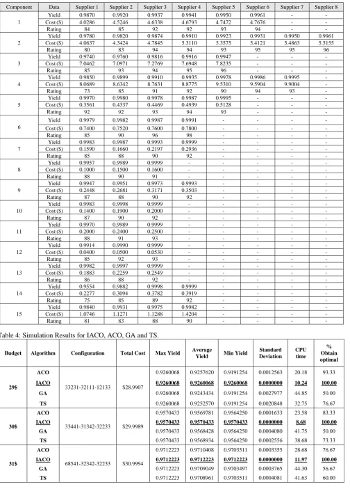
The numerical examples are performed by using the real data of one HDD model from an undisclosed HDD manufacturer. The selected HDD model consists of 15 components. The cost and yield of all components are shown in Table 3.

[image:4.595.305.551.540.701.2]

The important parameters for ACO and IACO are

α

,

β

and

ρ

. In order to search for the best configuration, the experiment is performed running the heuristics for each possible configuration 30 times. Each time, the run time is set to 30 seconds. The range for parameter

α

and

β

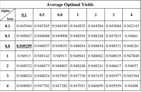
is [0.1,4]. The results are shown in Table 2.

Table 2: Average Optimal Yield for each alpha and beta.

The result from Table 2 shows that the best average yield is obtained when

α

is 0.1 and

β

is 0.8. This setting is used to find the best setting for

ρ

by running at different possible value in [0.01, 0.95] range. The result is shown in Fig 1. It can be seen that the range for suitable

ρ

is

Average Optimal Yields

Alpha beta

0.1 0.5 0.8 1 2 3 4

0.1 0.945946 0.945265 0.946349 0.944835 0.944584 0.943684 0.942143

0.5 0.949047 0.948688 0.949008 0.948549 0.948248 0.947815 0.94661

0.8 0.949299 0.948937 0.949035 0.948654 0.948654 0.948531 0.948281

1 0.94913 0.949142 0.94913 0.948941 0.948662 0.948635 0.947848

2 0.948332 0.948673 0.948803 0.948248 0.948241 0.946617 0.94657

3 0.948024 0.948024 0.947965 0.947736 0.947435 0.945977 0.945394

(5)

between 0.01 and 0.12. Once the value of

ρ

is greater than 0.12 the average optimum yields declines while the computational time increases. Hence, in the case study, the parameter setting used in ACO and ICO are 0.1 for 0.8 for

β

and 0.01 for

ρ

. Note that the value of

ρ

is arbitrary chosen.

[image:5.595.314.531.52.242.2]

For this study, three different available budgets ($27, $28 and $29) are considered. The sizes for the search space for these budgets are 11.19x106, 44.79x107 and 44.79x107 respectively and they was simulated using ACO, IACO, GA and TS to compare the best solution. Simulation results are shown as Table 4.

Fig. 1 Average Optimum Yield vs. Pheromone Evaporation of Trail

B. Simulation results

For all available budget settings ($27, $28, and $29), the best solutions are given in Tables 4. The results of each method show the best configurations to identify the best supplier of each component. Those are 33231-32111-12133, 33441-31342-32233, 68541-32342-32233 for the yield value at 0.9260068, 0.9570433 and0.9712223 and total component cost $28.9907, $29.9989and $30.9994 under the budget constraints $27, $28, and $29, respectively. The solution 33231-32111-12133 represents the first component comes from supplier 3, the second component comes from supplier 3, the third component comes from supplier 2 and so on. In addition, percentage of obtaining optimal solution for IACO are 100% for all budgets constraints while ACO, GA and TS are at 93.33 , 50.00, 76.67 for budget $29, 83.33, 50.00 , 73.33 for budget$30 and76.67, 56.67, 60.00 for budget$31 respectively. Also, average yield, standard deviation and computation time of IACO are lower than other heuristics in every budget settings. This means IACO algorithm is robust regardless of the budget setting.

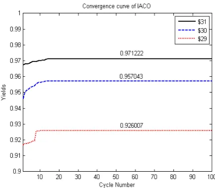
Using the simulation results, the best algorithm for this research in term of accuracy, robustness and computation time are IACO, ACO, TS and GA respectively. The convergence and effectiveness of IACO for different budget settings is shown in Fig 2.For all budget settings, IACO can achieve the optimal solution in less than 20 cycles. Moreover, it can be seen that as the available budget increases, the number of cycles used to reach the optimal solution also increases.

Fig. 2 Evolution of Best Solution for different available budgets using IACO

VIII.CONCLUSIONS

In this paper, four heuristics are proposed to solve HDD component yield optimization under budget and supplier’s rating constraints or YOBS problem. The problem is based on a series system (one piece per component) with multiple-choice constraints incorporated at each subsystem. This problem can be casted as a nonlinear binary integer programming problem and characterized as a NP-hard problem. Based on the design for assembling of each product, the formulation can be applied with different system. The result shows that Improved Ant Colony Optimization heuristic can solve realistic sized problem most efficiently when compared with Ant Colony Optimization, Genetic Algorithm and Tabu Search in terms of accuracy, robustness and computation effort.

REFERENCES

[1] Kwai Sang Chin, I-Ki Yueng and Kit Fai Pan. “Development of an assessment system for supplier quality management.” City University of Hong Kong, Kow Loon, Hong Kong, and the university of the West Indies, St Augustine, 2005

[2] Nourelfath M, Nahas N., “Quantized hopfield networks for reliability optimization.” Reliab Engng Sys Safety 2003;81:191–196.

[3] Nahas N and Nourelfath M, “Ant system for reliability optimization of a series system with multiple-choice and budget constraints”,

Reliability Engineering System Safety 2005;87: pp. 1–12.

[4] S.L. HO, Shiyou Yang, H.C. Wong, K.W.E Cheng and Guangzheng Ni., “An Improved Ant Colony Optimization Algorithm and Its Application to Electromagnetic Devices Designs.” IEEE Transactions on Magnetics, Vol 41, No.5, May 2005.

[5] J.H. Holland. “Adaptation in Natural and Artificial System. Ann Arbor, Michigan.” The University of Michigan Press, 1975.

[6] Coit DW, Smith A E., “Reliability optimization of series-parallel systems using a genetic algorithm.” IEEE Trans Reliab 1996;45(2): 254–60.

[7] Painton L, Campbell J., “Genetic algorithms in optimization of system reliability”. IEEE Trans Reliab 1995;44(2):172–8.

[8] Kwang Y.Lee. Mohamed A.EI-Sharkawi. Modern. “Heuristic Optimization Techniques Theory and Application to Power System.” Wiley Interscience, 2007, pp.38

[9] F.Glover. “Tabu Search Part I.” ORSA J. Comput, Vol.1 No.3, pp.190-206, 1989.

[image:5.595.47.291.211.376.2]

(6)

Table 3: Data of Test Problem

Component Data Supplier 1 Supplier 2 Supplier 3 Supplier 4 Supplier 5 Supplier 6 Supplier 7 Supplier 8 1

Yield 0.9870 0.9920 0.9937 0.9941 0.9950 0.9961 - - Cost($) 4.0286 4.5246 4.6338 4.6793 4.7472 4.7676 - -

Rating 84 85 92 92 93 94 - - 2

Yield 0.9780 0.9820 0.9874 0.9910 0.9923 0.9931 0.9950 0.9961 Cost($) 4.0637 4.3424 4.7845 5.3110 5.3575 5.4121 5.4863 5.5155 Rating 80 83 94 94 93 95 95 96 3

Yield 0.9740 0.9760 0.9816 0.9916 0.9947 - - - Cost($) 7.0462 7.0971 7.2769 7.6948 7.8235 - - -

Rating 85 93 94 95 96 - - - 4

Yield 0.9850 0.9899 0.9910 0.9935 0.9978 0.9986 0.9995 - Cost($) 8.0689 8.6342 8.7631 8.8775 9.5310 9.5904 9.9004 -

Rating 73 85 91 92 90 94 93 - 5

Yield 0.9970 0.9980 0.9978 0.9987 0.9995 - - - Cost($) 0.3561 0.4337 0.4469 0.4939 0.5128 - - -

Rating 92 92 93 94 93 - - - 6

Yield 0.9979 0.9982 0.9987 0.9991 - - - - Cost($) 0.7400 0.7520 0.7600 0.7800 - - - - Rating 85 90 96 98 - - - - 7

Yield 0.9957 0.9989 0.9999 - - - Cost($) 0.1000 0.1500 0.1600 - - - Rating 88 90 91 - - - 9

[image:6.595.50.555.68.772.2]

Yield 0.9840 0.9931 0.9975 0.9982 - - - - Cost($) 1.0746 1.1271 1.1288 1.4204 - - - - Rating 81 83 88 90 - - - -

Table 4: Simulation Results for IACO, ACO, GA and TS.

Budget Algorithm Configuration Total Cost Max Yield Average

Yield Min Yield

Standard Deviation

CPU time

% Obtain optimal

29$

ACO

33231-32111-12133 $28.9907

0.9260068 0.9257620 0.9191254 0.0012563 20.18 93.33 IACO 0.9260068 0.9260068 0.9260068 0.0000000 10.24 100.00

GA 0.9260068 0.9243434 0.9191254 0.0027977 44.85 50.00 TS 0.9260068 0.9252570 0.9191254 0.0020848 32.75 76.67

30$

ACO

33441-31342-32233 $29.9989

0.9570433 0.9569781 0.9564250 0.0001633 23.58 83.33 IACO 0.9570433 0.9570433 0.9570433 0.0000000 8.68 100.00

GA 0.9570433 0.9568428 0.9564250 0.0004080 41.75 50.00 TS 0.9570433 0.9568934 0.9564250 0.0002556 38.68 73.33

31$

ACO

68541-32342-32233 $30.9994

0.9712223 0.9710408 0.9703511 0.0003355 28.68 76.67 IACO 0.9712223 0.9712223 0.9712223 0.0000000 11.97 100.00