Programming Part for Robot Painter
Using Image Processing Algorithms Written in JAVA
Nodar MOMTSELIDZE* Zura SEKHNIASHVILI** Giorgi DARSALIA***
Abstract
Robot engineering is becoming one of the most popular field of artificial intelligence. Robots already can do the things which
were still impossible several years ago. They can play soccer, play music, think; play chess, fight, and can do much, much more. This article is dedicated to the problem of creating program (written in java) when embedded in a robot’s logic board, would en-able it to paint. This is a program which scans the image pixel by pixel and draws another image which is an outline of the original image.Keywords:image processing; Canny edge detection; Gaussian smoothing
Introduction
The following article describes how to convert image tak-en by camera into an image which contains only the edges of the original image, how to extract all edge coordinates from produced image and save them in memory and how to draw only the edges of the original image using saved coordinates. The article also describes image processing in detail using sev-eral famous algorithms.
The following algorithms are used 1. Image processing.
2. Edge detection. 3. Gaussian Smoothing.
Realization
The source image (relative or full) path as a string is sup-plied to the program. It creates image from this path and starts processing it at the moment the program is run. Using an edge detection algorithm (in our case “Canny Edge Detection” see explanation below) the program processes the original image and creates a new image (which contains only black edges (all colorful edges are converted into black) of original image on white background) and integer array which contains the infor-mation about image pixels. The array is one dimensional with the length of image width multiply by image height. It contains information whether image pixel is black or white. The array’s first image width elements contain information about pixels on the 1st horizontal line (from the top) of image, the next image width elements of array contain information about pixels on the 2nd horizontal line of image and so on…
The constructor of ImageDraw class. ImageDraw(String fileLocation){ . . . .
CannyEdgeDetector detector = new CannyEdgeDetec-tor();
. . .
detector.setSourceImage(image); detector.process();
//edges is instance of BufferedImage class. edges = detector.getEdgesImage();
// data is one dimensional array data = detector.getData(); }
The variable edge is actually the image which is drawn by a program. In case of interrupting the program here and draw-ing this image on canvas, usdraw-ing graphics.drawImage() method the result would be the same for the following program, but the point is that we are not interested in drawing this image on computer screen.
Our aim is to embed this program into a robot’s “brain” in order that the robot will be able to draw the images on paper. For this purpose, the program needs to know all coordinates of the image edges, which we need to find out. So we move to the next step of the program.
We introduce a new algorithm to process the array of data. The array contains information about all pixels of “image of edges”, -1 means the pixel is black and in other case the pixel is white. For example: The image dimensions are 480x600 and we are referring to 500th element of the data array. This means that we are talking about pixel of image at coordinates (x is reminder of 500 divided by 480 and y is the integer of 500 divided by 480. x = 20 and y = 1) 20x1 from top-left corner (x is from left, y is from top).
It saves the coordinate in LinkedList and “follows detected point” (using followLine method). It checks every neighbor-hood points of detected point and as it finds black pixel it saves the coordinates again. This process continues till the program finds black pixels in the neighborhood of previous detected pixel. If the program could not find black pixel it continues horizontal scanning from the first detected pixel until it finds another one.
This method scans whole image and saves all coordinates in a List.
The last step is to output edges. Right now the output im-age is drawn on computer screen but our purpose is getting output image on paper or on a board. That’s why we created abstract class “Painter” with abstract methods: “penUp”, “pen-Down”, “moveTo” which are implemented for java PCanvas (as the output image is drawn on Canvas), but later they will be implemented for robot as drawing orders. We have also “penI-sUp” Boolean variable (using which we check if the program is in drawing process or not), “curx” and “cury” integer vari-ables which refers to current pen position. We have additional “rmoveTo” abstract method (which increments “curx” and “cury” variable which “incrx” and “incry” method parameters), “MAXX” and “MAXY” properties (drawn image width and height).
Here is an implementation of abstract class Painter.
These steps are essential for the program, as CannyEdge-Detection is used in ImageDraw constructor and drawing methods, such as “penUp”, “penDown”, “moveTo” and others are implemented in PainterAWT class.
Here is an implementation of drawing image using data ar-ray coordinates. “r” variable is an instance of Artist class (class which contains the main method).
Implementation of followLine method, which generates abstract commands.
Journal of Technical Science and Technologies; ISSN 2298-0032
Canny Edge Detector
The Canny edge detector is an edge detection operator that uses a multi-stage algorithm to detect a wide range of edges in images. It was developed by John F. Cannyin 1986. Canny also produced a computational theory of edge detection explaining why the technique works.
The Canny operator was designed to be an optimal edge detector (according to particular criteria --- there are other detectors around that also claim to be optimal with respect to slightly different criteria).
How It Works?
The Canny operator works in a multi-stage process. First of all the image is smoothed by Gaussian convolution. Then a simple 2-D first derivative operator (somewhat like the Roberts Cross) is applied to the smoothed image to highlight regions of the image with high first spatial derivatives. Edges give rise to ridges in the gradient magnitude image. The algorithm then
tracking process exhibits hysteresis controlled by two thresh-olds: T1 and T2, with T1 > T2. Tracking can only begin at a point on a ridge higher than T1. Tracking then continues in both directions out from that point until the height of the ridge falls below T2. This hysteresis helps to ensure that noisy edges are not broken up into multiple edge fragments.
Guidelines for Use
The effect of the Canny operator is determined by three parameters --- the width of the Gaussian kernel used in the smoothing phase, and the upper and lower thresholds used by the tracker. Increasing the width of the Gaussian kernel reduces the detector’s sensitivity to noise, at the expense of losing some of the finer detail in the image. The localization error in the detected edges also increases slightly as the Gaussian width is increased. Usually, the upper tracking threshold can be set quite high, and the lower threshold quite low for good results. Setting the lower threshold too high will cause noisy edges to break up. Setting the upper threshold too low increases the number of spurious and undesirable edge fragments appearing in the output.
Development of the Canny Algorithm
Canny’s aim was to discover the optimal edge detection algorithm. In this situation, an “optimal” edge detector means:
• good detection – the algorithm should mark as many real edges in the image as possible.
• good localization – edges marked should be as close as possible to the edge in the real image.
• minimal response – a given edge in the image should only be marked once, and where possible, image noise should not create false edges.
To satisfy these requirements Canny used the calculus of variations – a technique which finds the function that optimizes a given function. The optimal function in Canny’s detector is described by the sum of four exponential terms, but it can be approximated by the first derivative of a Gaussian.
Stages of the Canny Algorithm
Noise Reduction
Because the Canny edge detector is susceptible to noise present in raw unprocessed image data, it uses a filter based on a Gaussian (bell curve), where the raw image is convolved with a Gaussian filter. The result is a slightly blurred version of the original which is not affected by a single noisy pixel to any significant degree.
Finding the Intensity Gradient of the Image
An edge in an image may point in a variety of directions, so the Canny algorithm uses four filters to detect horizontal, vertical and diagonal edges in the blurred image. The edge de-tection operator (Roberts, Prewitt, Sobel for example) returns a value for the first derivative in the horizontal direction (Gx) and the vertical direction (Gy). From this the edge gradient and direction can be determined:
The edge direction angle is rounded to one of four angles representing vertical, horizontal and the two diagonals (0, 45, 90 and 135 degrees for example).
Non-maximum Suppression
Given estimates of the image gradients, a search is then carried out to determine if the gradient magnitude assumes a local maximum in the gradient direction. So, for example, • if the rounded gradient angle is zero degrees (i.e. the edge is in the north-south direction) the point will be considered to be on the edge if its gradient magnitude is greater than the mag-nitudes at pixels in the north and south directions,
• if the rounded gradient angle is 90 degrees (i.e. the edge is in the east-west direction) the point will be considered to be on the edge if its gradient magnitude is greater than the magni-tudes at pixels in the west and east directions,
• if the rounded gradient angle is 135 degrees (i.e. the edge is in the north east-south west direction) the point will be con-sidered to be on the edge if its gradient magnitude is greater than the magnitudes at pixels in the north east and south west
directions,
• if the rounded gradient angle is 45 degrees (i.e. the edge is in the north west-south east direction)the point will be con-sidered to be on the edge if its gradient magnitude is greater than the magnitudes at pixels in the north west and south east
directions.
From this stage referred to as non-maximum suppression, a set of edge points, in the form of a binary image, is obtained. These are sometimes referred to as “thin edges”.
Tracing Edges through the Image and Hysteresis
Thresholding
Large intensity gradients are more likely to correspond to edges than small intensity gradients. It is in most cases impos-sible to specify a threshold at which a given intensity gradi-ent switches from corresponding to an edge into not doing so. Therefore Canny uses thresholding with hysteresis.
Thresholding with hysteresis requires two thresholds – high and low. Making the assumption that important edges should be along continuous curves in the image allows us to follow a faint section of a given line and to discard a few noisy pixels that do not constitute a line but have produced large gra-dients. Therefore we begin by applying a high threshold. This marks out the edges we can be fairly sure are genuine. Starting from these, using the directional information derived earlier, edges can be traced through the image. While tracing an edge, we apply the lower threshold, allowing us to trace faint sections
of edges as long as we find a starting point.
Once this process is complete we have a binary image where each pixel is marked as either an edge pixel or a non-edge pixel. From complementary output from the non-edge trac-ing step, the binary edge map obtained in this way can also be treated as a set of edge curves, which after further processing can be represented as polygons in the image domain.
Differential Geometric Formulation of the Canny
Edge Detector
A more refined approach to obtain edges with sub-pixel ac-curacy is by using the approach of differential edge detection, where the requirement of non-maximum suppression is formu-lated in terms of second- and third-order derivatives computed from a scale space representation (Lindeberg 1998) – see the article on edge detection for a detailed description.
Variational-Geometric Formulation of the
Haral-ick-Canny Edge Detector
A variational explanation for the main ingredient of the Canny edge detector, that is, finding the zero crossings of the 2nd derivative along the gradient direction, was shown to be the result of minimizing a Kronrod-Minkowski functional while maximizing the integral over the alignment of the edge with the gradient field (Kimmel and Bruckstein 2003). See ar-ticle on regularized Laplacian zero crossings and other optimal edge integrators for a detailed description.
Gaussian Smoothing
The Gaussian smoothing operator is a 2-D convolution operator that is used to `blur’ images and remove detail and noise. In this sense it is similar to the mean filter, but it uses a different kernel that represents the shape of a Gaussian (`bell-shaped’) hump. This kernel has some special properties which are detailed below.
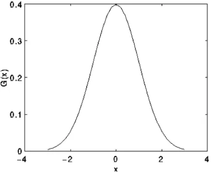
The Gaussian distribution in 1-D has the form:
where
σ
is the standard deviation of the distribution. We have also assumed that the distribution has a mean of zero (i.e. it is centered on the line x=0). The distribution is illustrated in Figure 1.In 2-D, an isotropic (i.e. circularly symmetric) Gaussian has the form:
This distribution is shown in Figure 2.
Journal of Technical Science and Technologies; ISSN 2298-0032
In theory, the Gaussian distribution is non-zero every-where, which would require an infinitely large convolution ker-nel, but in practice it is effectively zero more than about three standard deviations from the mean, and so we can truncate the kernel at this point. Figure 3 shows a suitable integer-valued convolution kernel that approximates a Gaussian with a
σ
of 1.0.Figure 3: Discrete approximation to Gaussian function with
σ=1.0
Once a suitable kernel has been calculated, then the
ian shown above is separable into x and y components. Thus the 2D convolution can be performed by first convolving with a 1D Gaussian in the x direction, and then convolving with another 1D Gaussian in the y direction. (The Gaussian is in fact the only completely circularly symmetric operator which can be decomposed in such a way.) Figure 4 shows the 1D x component kernel that would be used to produce the full kernel shown in Figure 3 (after scaling by 273, rounding and truncat-ing one row of pixels around the boundary because they mostly have the value 0. This reduces the 7x7 matrix to the 5x5 shown above.). The y component is exactly the same but is oriented vertically.
Figure 4: One of the pair of 1-D convolution kernels used to calculate the full kernel shown in Figure 3 more quickly.
A further way to compute a Gaussian smoothing with a large standard deviation is to convolve an image several times with a smaller Gaussian. While this is computationally com-plex, it can have applicability if the processing is carried out using a hardware pipeline.
The Gaussian filter not only has utility in engineering ap-plications. It is also attracting attention from computational biologists because it has been attributed with some amount of biological plausibility, e.g. some cells in the visual pathways of the brain often have an approximately Gaussian response.
Conclusion
The Canny algorithm is adaptable to various environ-ments. Its parameters allow it to be tailored to recognition of edges of differing characteristics depending on the particular requirements of a given implementation. In Canny’s original paper, the derivation of the optimal filter led to a Finite Im-pulse Responsefilter, which can be slow to compute in the spa-tial domain if the amount of smoothing required is important (the filter will have a large spatial support in that case). For this reason, it is often suggested to use Rachid Deriche’s infinite impulse response form of Canny’s filter (the Canny-Deriche detector), which is recursive, and which can be computed in a short, fixed amount of time for any desired amount of smooth-ing. The second form is suitable for real time implementations in FPGAs or DSPs, or very fast embedded PCs. In this context, however, the regular recursive implementation of the Canny operator does not give a good approximation of rotational sym-metry and therefore gives a bias towards horizontal and vertical edges.
References
[1] Canny Edge detector:
http://en.wikipedia.org/wiki/Canny_edge_detector
[2] 2004 Robert Fisher, Simon Perkins, Ashley Walker, Erik Wolfart, Image processing Learning resources HIPR2 explore with JAVA, http://homepages.inf.ed.ac.uk/rbf/HIPR2/hipr_top. htm
Contents and Index > Canny Edge Detector
[3] 2004 Robert Fisher, Simon Perkins, Ashley Walker, Erik Wolfart, Image processing Learning resources HIPR2 explore with JAVA, http://homepages.inf.ed.ac.uk/rbf/HIPR2/hipr_top. htm
Contents and Index > Gaussian Smoothing