On the relation between equation formulation of constrained systems and implicit numerical integration and optimization

University of Twente

Faculty of Electrical Engineering

On the relation between equation formulation of

constrained systems and implicit

numerical integration and optimization

P.A.J. Koenders M.Sc. Thesis

Supervisors: Prof. dr. ir. J. van Amerongen Dr. ir. P. C. Breedveld Ir. G. Golo

Summary

The aim of this study is to establish the relation between the implicit numerical integration process and control or optimization problems. The iteration process of the implicit numerical methods and

Table of contents

Summary... 2

Nomenclature... 4

Preface ... 5

1 Introduction ... 6

2 State of art in formulating systems with constraints... 7

2.1 Introduction ... 7

2.2 Implicit port-controlled Hamiltonian description of systems... 8

2.3 Index of system and stiffness of system... 9

2.4 Formulation, dynamical behavior and computational efficient... 12

2.5 Examples ... 14

2.5.1 Bond graph model with dependent state, derive index 1 and 2 system ... 14

2.5.2 Elimination dependent state by adding spring and damper... 17

2.5.3 Elimination dependent state by symbolic index reduction ... 20

2.6 summary... 21

3 Implicit integration methods... 23

3.1 Introduction ... 23

3.2 Numerical techniques for implicit integration methods ... 23

3.2.1 Polynomial basis ... 23

3.2.2 Modified Newton iteration... 25

3.2.3 Step size control... 26

3.2.4 Flow chart ... 26

3.3 Summary ... 29

4 Index reduction, a control approach ... 30

4.1 Introduction ... 30

4.2 Non-linear control ... 30

4.3 Control design ... 32

4.3.1 Feedback linearization ... 32

4.3.2 Nonlinear controller ... 33

4.3.3 Stabilization investigation... 35

4.3.4 Stabilization of the constraint manifold ... 36

4.3.5 Implementation ... 38

4.4 Example... 39

4.4.1 Stabilization investigation... 40

4.5 Conclusions ... 42

5 Implicit numerical methods and Index reduction, a comparison... 43

5.1 Introduction ... 43

5.2 Comparison of numerical techniques... 43

5.3 Comparison by means of simulation... 46

5.3.1 Flyball governor model... 46

5.3.2 Simulation results... 52

5.3.3 Summary ... 63

5.3.4 Conclusion ... 64

6 Conclusions and recommendations ... 65

6.1 Conclusions ... 65

6.2 Recommendations ... 65

Appendix A: Implementation Feedback linearization and projection algorithm... 66

Nomenclature

z Vector of algebraic variables.

u

Vector of exitation variables.

λ

Vector of semi-state variables. (Lagrange multiplier)

x

State vector of energy variables: volume, charge, flux, displacement, momenta, etc.

H( )

x

Total energy of system. [J]

f eR_, R _{Vectors power variables corresponding to R-ports.}

Φ

Vector of constraint variables.

M Mass

p Momentum of mass M

Preface

This project is the last part of my masters education at the university of Twente carried out at the department of Electrical Engineering in the Control Laboratory group. I followed the education part-time. Four days a week I was working at Witteveen+Bos in Deventer and one day a week I was working on my masters education. This is the reason why it took two years to complete this project. Peter Breedveld is the supervisor of the project. The first year we almost weekly discussed the progress of the project. The second year Goran Golo joined the progress discussions. The discussions where instructive and pleasant. I would like to thank them for their critical view and ideas that improved the work.

1

Introduction

Computer simulation is an important engineering tool because it can be used to analyze engineering problems and it can be used for control design. Computer simulation is used in areas like chemical process engineering, robotic arm manipulators, ground vehicles, space aircraft and electrical circuits engineering. In general nonlinear constrained systems can be formulated in different ways depending on the numerical techniques the modeler wants to use. When the nonlinear constrained system is described by means of Differential Algebraic Equations (DAE) we can use an implicit integration methods to find the solution (Gear, 1971), (Petzold, 82). When the DAE is transformed into Ordinary Differential Equations (ODE) we can use explicit integration methods in order to fined the solution (Ascher, 1996), (Golo, 2000). The applied numerical technique, the way of implementation and the way that the equations are formulated determine the numerical efficiency, the reliability and the accuracy of the computer simulation.

The aim of this study is to formulate the implicit numerical integration process, i.e. the iteration process that minimizes the error, in terms of a control or rather optimization problem. The quantity to be integrated need to be adapted in such a way that the output satisfies the imposed constraint that causes the dependence between the storage ports. By comparing and evaluating the possible formulation techniques a relation is to be found between this problem and the way in which the discipline of modern control theory solves optimization problems.

Chapter 2 contains an inventory of the state of art ways of formulation of constrained

nonlinear systems. The dynamical properties of the different ways of formulation are investigated and the applicable numerical techniques are investigated. Next the basic numerical techniques and

implementation strategies of implicit integration methods are studied. The results are reported in chapter 3. The obtained knowledge will be used to develop control strategies. In chapter 4 the

available nonlinear control strategies are studied in order to find a suitable method to solve the control and optimization problem of the implicit integration method. In chapter 5 the proposed control and optimization strategy is compared with the implicit integration method. After studying the available nonlinear control strategies we find that Index reduction by means of feedback linearization and stabilization of the constraint manifold by means of the projection algorithm is a suitable alternative for implicit integration methods. Because a system that is controlled by means of feedback

2

State of art in formulating systems with

constraints

2.1

Introduction

There are a number of ways to make a graphical description of a physical system (Ideal Physical Model (IPM), Bond Graph Model (BGM), Block Diagram Model (BDM)). In this study we will take the bond graph model representation as an example. Using the bond graph technique we can make a graphical representation of physical systems that is called bond graph model. The bond graph model represents a multiport system involving energy flows (Paynter, 1961), (Breedveld, 1985). When we have obtained the bond graph model we can write down the algebraic state space equations of the junctions. The equations describing the bond graph model correspond to implicit port-controlled Hamiltonian systems (Golo, 2000). In this study we will describe the bond graph models as port-controlled Hamiltonian systems (PCH) (Van der Schaft, 2000). In this study non-linear constrained physical systems are concerned. Systematic procedures for constructing graphical models from constrained physical systems lead to models containing dependent states. The equations that are derived are Differential Algebraic Equations (DAE). DAE can be solved by means of implicit integration methods. Another option is to eliminate the dependent states from the graphical model. In case of a bond graph model the dependent states can be eliminated by transformation of junction structure (Golo, 2000). In general the equations that are derived from this modified bond graph model is an Ordinary Differential Equation (ODE) with an invariant (Ascher, 1996). This invariant can cause inaccuracy of the numerical simulations. In this chapter we will discuss methods to formulate and modify bond graph models that are obtained from constrained mechanical systems and how equations can be derived and modified.

The way that the bond graph model and the equations are formulated determines the

dynamical properties of the system. How a constrained system is formulated depends on the needs of the modeler. For example, if we need a simulation model for real-time simulation, the constrained system should be transformed into an explicit system.

The dynamical properties are usually expressed by the eigenvalues of the linearized system. In other words, the position of the eigenvalues determines what type of numerical techniques should be used. For example, if the real parts of the eigenvalues differ largely (such type of system is called stiff system) then the explicit integration techniques don't give good results.

one or two, and some additional conditions are satisfied, then implicit numerical techniques give good results. Otherwise, techniques for index reduction have to be applied.

In this chapter we will discuss the definition of the index of a system and the definition of a stiff system. In order to give some insight in the dynamical properties of the systems in relation to the method of formulation we will use a linear mechanical system as an example.

2.2

Implicit port-controlled Hamiltonian description of systems

When we have obtained a bond graph model from a constrained mechanical system, we can write down the equations. The port-controlled Hamiltonian (PCH) description of a bond graph model is given by (Golo, 2000):

& (

x J x

x x G x G x f G x u

= C ₎

∂

H_{( )}+ _{( )} + C,R_{( )} R + C,U_{( )}

∂

λ

, (2.1)

0=G x

x x T

( )

∂

H( )

∂

, (2.2)

e G x

x x G x u R _{= −(} C,R_{( ))}T

∂

H_{( )+} R,U_{( )}

∂

, (2.3)

Ω

( R, R, )

f e x =0, (2.4)

y G x

x x G x f J x u

= −( C,U( ))T

∂

H( ) (− R,U( ))T R + U( )

∂

, (2.5)

whereJ xC_{( )and J x}U_{( ), are skew-symmetric matrices, G x( )is a full rank matrix for}

∀ ∈

x

χ

_.

x

_is

the state vector (vector of energy variables: volume, charge, flux, displacement, momenta etc.).

χ

is the manifold of variables. H( )

x

is the total energy of system, f eR R

, are the power variables corresponding to R-type of ports and

Ω

is an algebraic function such that every pair f eR R

, satisfying (2.4) satisfies also the inequality f R₍eR ₎T _≥0.

In many cases the map

Ω

is linear and when we have an energy dissipating system we can express (2.4) as

fR ₌ R x e_{( )} R

Where R x( ) is a positive definite matrix, then system (2.1)-(2.4) becomes

& ( ( ) )

( )

x J x G x R x G x

x x G x

G x G x R x G x u

= − + +

−

C C,R C,R T

C,U C,R R,U ( ) ( )( ( )) H( ) ( )

( ) ( ) ( ) ( ) ,

∂

∂

λ

(2.6)

0=G x

x x T

( )

∂

H( )

Let G x⊥( ) be a maximum rank matrix so that

G x G x

⊥( ) ( )= 0. Sine

G x

( ) is a constant rank matrix then

G x

⊥_{( ) is also a constant rank matrix. Premultiplying (2.1) by G x}⊥_{( ) the following system of}

equations is obtained. G x x G x J x

x x G x G x f G x G x u

⊥_{( ) =} ⊥_{( )} C ₎ H_{( )+} ⊥_{( )} C,R_{( )} R ₊ ⊥_{( )} C,U_{( ) ,}

& (

∂

∂

(2.8)

0=G x

x x T

( )

∂

H( )

∂

(2.9)

e G x

x x G x u R _{= −(} C,R_{( ))}T

∂

H_{( )+} R,U_{( ) ,}

∂

(2.10)

Ω

(_{f e x}R, R, )_{=0. (2.11)}

Similarly if f R ₌ R x e_{( )} R _{the system (2.8)-(2.11) becomes} G x x G x J x G x R x G x

x x G x G x G x R x G x u

⊥ ⊥

⊥

= − +

−

( ) ( ) ( ) ( )( ( )) H( ) ( ) ( ) ( ) ( ) ( ) ,

C C,R C,R T

C,U C,R R,U

& ( ( ) )

( )

∂

∂

(2.12)

0=G x

x x T

( )

∂

H( )

∂

(2.13)

2.3

Index of system and stiffness of system

Index of system:

The index of constrained system characterizes the behavior of the numerical solution and is a measure of the singularity, how much constrained system differs from an ODE. In the following text the definition of the local differential index, index two system and index one system is given (Ascher, 1998);

Local differential indexConsider a system described by the following implicit equation

F z z u( , , )=& 0 (2.14)

Equation (2.14) has a local differential index m at the point ( , )z u0 0 if m is the minimal number such

that there exists a neighborhood of the point ( , )z u0 0 in which the system of equations

F z z u( , , )=& 0, d ( , , )

dt = F z z u&

0,

M

d ( , , )

dt =

m m F z z u&

0,

When (2.3) is inserted in (2.4), the set of equations (2.1)-(2.4) becomes

& (

x J x

x x G x G x f G x u

= C ₎

∂

H_{( )}+ _{( )} + C,R_{( )} R + C,U_{( ) ,}

∂

λ

(2.15)

0=G x

x x T_{( )}

∂

H_{( )}

∂

, (2.16)

~

, .

Ω

( R, )

f x u =0 (2.17)

Proposition [Index two system]Consider system described by (2.15)-(2.17). Assume that for x = x0

and u=u0 equation (2.16) is satisfied and that there exists f0

R _{such that (2.17) is satisfied. If} det

∂

∂

∂

∂

xT G x x x G x T

x x ( ) H( ) ( )        ₌ ≠ 0

0, (2.18)

det ~

∂

∂

Ω

( , , ) ( ) R

R T _{x x} f f u u

R R

f x u f       ₌ ≠ = = 0 0 0

0, (2.19)

then the system (2.15)-(2.17) has a differential index two at the point ( ,_{x f} R, , )_u

0 0

λ

0 0 .

Proof: In this case z=( ,x

λ

_,f R)_{. Differentiating of (2.17) gives}

∂

∂

λ

~

& _{( , ,}

Ω

( , , )

( ) , )

R R T

R R

f x u

f f +L x u1 f =0

Now it is clear that if the condition (2.19) is satisfied then the last equation can be solved for f&R

. Differentiating (2.16) gives

∂

∂

∂

∂

λ

λ

xT G x x x G x L x u f

T R

( ) H( ) ( ) 

  + 2( , , ,& )=0

If condition (2.18) is satisfied then the last equation can be uniquely solved for

λ

. Therefor for the given value of x f u0, 0 , 0 0

R

,

λ

can be uniquely computed. Differentiating of the last equation gives

∂

∂

∂

∂

λ

λ

xT G x x x G x L x f u u

T R

( ) H( ) ( ) 

  &+ 3( , , , ,&)=0.

Similarly, we can consider the following system (

λ

is eliminated). G x x G x J x

x x G x G x G x G x f G x G x u

⊥_{( ) =} ⊥_{( )} C ₎ H_{( )+} ⊥_{( ) ( ) +} ⊥_{( )} C,R_{( )} R ₊ ⊥_{( )} C,U_{( ) ,}

& (

∂

∂

λ

(2.20)

0=G x

x x T

( )

∂

H( )

∂

(2.21)

~

, .

Ω

(_{f x u}R, )_{=0 (2.22)}

Proposition [Index one system] Consider the system described by (2.20)-(2.22). Assume that for

x= x0 and u= u0 equation (2.21) is satisfied and that there exists f0

R _{such that (2.22) is satisfied.} If the conditions (2.18) and (2.19) are satisfied then the system (2.20)-(2.22) has a differential index one at the point ( , R, )

x f u0 0 0 .

Proof: In this case z=( ,x f R)

. The part of the proof regarding the calculation of f&R

is the same as in the proof of the index-two system. Now, we concentrate on calculation of x_&. Differentiating (2.21) and regrouping the derivatives of the left side gives the following

G x

x G x x x

x L x f u

⊥



 



  



   = ( )

( ) H( ) T

T R

∂

∂

∂

∂

& 4( , , ) .

If the condition (2.18) is fulfilled then the rank of the matrix on the left side is full ∀ ∈x

χ

. For proving this, the following identity is used

( )

(

)

rank A rank rank

B A BA

   



= + ⊥

Stiffness of system:

The stiffness of a system is defined by Lambert (1980). This definition is modified by Van Dijk, (1994).

Lambert (1980), defines stiff systems in the following way: Consider the common system of ODE of the form:

& ( )

y

=

Ay

+

φ

( ) ,

x y

φ

x ∈ℜm _(2.23)

This system is said to be stiff if: 1.

Re( )

λ

_i <

0

,

i

=

1 2

, ,..,

n

and

2.

max Re( ) min Re( )

i i

i i

S

λ

λ

= >>1,

where

λ

_i is the eigenvalue of matrix A∈ℜm,

Re( )

λ

_i is the real part of

λ

_i and S is called the "stiffness ratio".

A nonlinear system

y

&

=

f x )

( ,

y

is said to be stiff, on an interval I of x, if for

∀

x

∈

I the eigenvalues

λ

( )

x

of the Jacobian

∂ ∂

f

/

y

satisfy 1 and 2 above.

The previous definition is refined by Van Dijk, as follows:

A system described by (2.23) is stiff if h. / y

∂ ∂

f >>1 where h represents the step size of the applied integration method.

2.4

Formulation, dynamical behavior and computational efficient

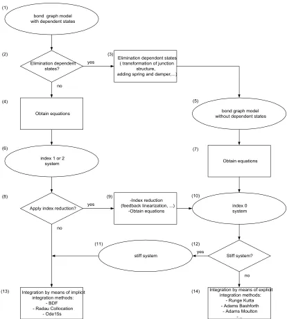
Systematic procedures for constructing bond graph models from physical systems lead to bond graph models containing dependent states. The dependent states can be eliminated by means of model modification or symbolic reduction of the constraint. The equation that is derived from the bond graph model with constraints is usually index 1 or 2. The equation that is derived from the bond graph model without dependent states is index 0. An explicit integration method can be used is the index is reduced to zero. When the index is one or two we must use an implicit integration method. The stiffness is also a property that determines the choice of integration method. When the index of the system is zero and the system is stiff we must use an implicit integration method. Figure 1 shows the graphical

bond graph model with dependent states

bond graph model without dependent states

index 1 or 2 system

index 0 system Elimination dependent states

( transformation of junction structure, adding spring and damper,...) Elimination dependent

states?

Obtain equations

Apply index reduction?

-Index reduction (feedback linearization, ...)

-Obtain equations

Stiff system?

Integration by means of implicit integration methods:

- BDF - Radau Collocation

- Ode15s

Integration by means of explicit integration methods:

- Runge Kutta - Adams Bashforth

- Adams Moulton - .. Obtain equations yes

no

yes

no (1)

(2) (3)

(4) (5)

(6) (7)

(8) (9) (10)

(13)

(12)

(14) yes

no stiff system

(11)

Figure 1 : Graphical representation of the formulation of constrained system

The formulation of constrained mechanical systems. • (1) Bond graph model with dependent states:

The kinematc constraints will cause dependent states in the bond graph model. • (5) Bond graph model without dependent states:

The kinematic constraints that are present in the bond graph model can be eliminated by means of, for example, geometric junction transformation (Golo, 2000) or adding spring and damper (3). • (6) Index 1 or 2 system:

• BDF (Gear, 1971) the Dassl (Petzold, 1982) implementation is used in 20 Sim and the Ode15s implementation (Shampine,2000) is used in Matlab.

• Radau Collocation (Ascher, 1998). • (10) Index 0 system:

The equation obtained from the bond graph model without a dependent state is index 0. The index 1 or 2 system (6) can be transferred into an index 0 PCH system by means of index reduction (9). An example of index reduction is feedback linearization that will be discussed in chapter 4. The index 0 system can be solved by means of explicit integration methods (14) like Runge Kutta, Adams Bashforth, Adams Moulton (Ascher, 1998), (Gear, 1971).

• (11) Stiff system:

A stiff index 0 system can't be solved by means of an explicit integration methods (Ascher, 1998). A stiff index 0 system has to be solved by means of an implicit integration method.

The Flow chart that is presented in Figure 1 can help the modeler in order to find the needed formulation strategy. The flow chart could be implemented in a Decision Support System (DSS).

2.5

Examples

In this subchapter we will show how to obtain and modify a bond graph model and how to derive equations. We will use a gear wheels system as an example. The bond graph model, which is obtained from the concerned Gear wheels system, has a dependent state. The derived equations can be

formulated as an index 1 or as an index 2 system. The dependent states can be eliminated by adding spring and damper or by symbolic reduction of the constraint. The dynamical behavior will be investigated by analyzing the location of the eigenvalues.

2.5.1 Bond graph model with dependent state, derive index 1 and 2 system

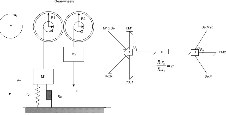
Figure 2 shows the linear mechanical system that consists of winches. The winches are transitionally fixed and can rotate only. The masses are subject to gravity and can be translated vertically. There is an external force F that acts on

M

₂. The winches and the cables are modeled as massless. The loads are modeled as point masses. The masses are kinematically coupled. There is one kinematic constraint. The difference between the velocities of the masses

M

₁ and

M

₂ is R

r v

R r v

1 1

1

2 2

2

= − and therefore

I:M2 Gear-wheels R1 _R2 r1 r2 M1 M2

C1 _Rc F

V+ w+ 1 TF .. C:C1 Rc:R M1g:Se I:M1

−R r = R r n

1 2 2 1

v

₁ 1 Se:M2g Se:F

v

₂

Figure 2 : Gear Wheels: Ideal physical model and bond graph model.

The state vector is

[

]

x

T

=

p

x p

∈

1 2

χ

,

where

p

₁ and

p

₂are the momenta of masses

M

₁ and

M

₂, respectively x is the position of mass

M

₁

and

χ

= ℜ

3_{. The state x is independent. One of the states}

p

1 and

p

2 is dependent and the other is

independent. In this case the state

p

₁ is chosen independent and

p

₂ is chosen dependent.

The total energy is given by.

H p

M

p

M C x

( )x = 1 + +

2 1 2 1 2 1 1 2 1 2 2 2 1 2

The equations (2.1)-(2.4) describe this system where,

JC_{( )}x ₌

−          

0 1 0

1 0 0

0 0 0

,

G x

( )

=

−

         

n

0 1

,

G

C R,

( )

x

=

          1 0 0 , (2.24)

[

]

G

R U,

( )

x

=

_{0 0 0 ,}

G

C U,

( )

x

=

          1 0 0 0 0 0 0 1 1

,

u

=

         

M g

M g

F

1

2 ,

G

⊥

x

=













( )

1 0

0 1 0

n

(2.25)

Ω

(

R

,

R

, )

R

R

c R

Index 2 system:

Because (2.18) and (2.19) are satisfied ∀ ∈x

χ

the equations can be formulated as an index 2 system, given by

&

( )

x

x

x

=

−

−





















+

−





















+









































R

H

n

M g

M g

F

c

1 0

1

0

0

0

0

0

0

1

1 0 0

0 0 0

0 1 1

1 2

∂

∂

λ

[

]

0

=

n

0

−

1

∂

H

∂

( )

x

x

.

Index 1 system:

Since G x⊥_{( ) is a maximum rank matrix such that G x G x}⊥_{( ) ( )=0 then the previous system can be}

rewritten as

1 0

0 1 0

0 0 0

1

0

1

0

0

0

1

1

0 0 0

0 0 0

1 2 1 1 1 2 2 1 2

n p

x

p

R

n

p

M

x

C

p

M

n n M g

M g

F

c









































=

−

−

−

























































+









































&

&

&

(2.27)

Here, the first two rows represent the differential equations and the third row represents the algebraic equation.

Eigenvalues:

System (2.27) is described by

Ex

&

=

Ax Bu

+

. Suppose the rank of

E

is m and

m n

≤

where n is the dimension if the matrix

A

. Then m eigenvalues of the system

Ex

&

=

Ax Bu

+

are the root of the following equation

det(

λ

E Ax

−

)

=

0

The rest n-m are placed in − ∞. In this case

E

=





















1 0

0 1 0

0 0 0

n

and

A

=

−

−

−





































R

M

C

M

M

M

n

c 1 1 1 2 1

1

0

1

0

0

0

1

(

1 2

)

2 1 0

1 1 1

+ +



 



 + =

n R

M M C

c

λ

λ

Since m=2 and n=3 the third eigenvalue is

−∞

.

λ

1

= −∞

λ

2 3,

= −

0 0025 1118

,

±

,

.i

The numerical values, which are used to calculate the eigenvalue, are;

n

R r

R r

= −

1 2

=

2 1

1

,

M

₁

=

M

₂

=

5 kg, Rc = 0.05 N/

m

2_{, C1 = 0.08 N/m, Cp = 1E-5 N/m and Rp = 1000N/}

m

2_{, F=1 N,}

g=1 N/kg..

Stiffness ratio:

We can calculate the stiffness ratio by means off

S i i

i i

= max Re( ) = ∞ = ∞

min Re( ) ,

λ

λ

0 0025

Because S>>1, (2.27) is a stiff system.

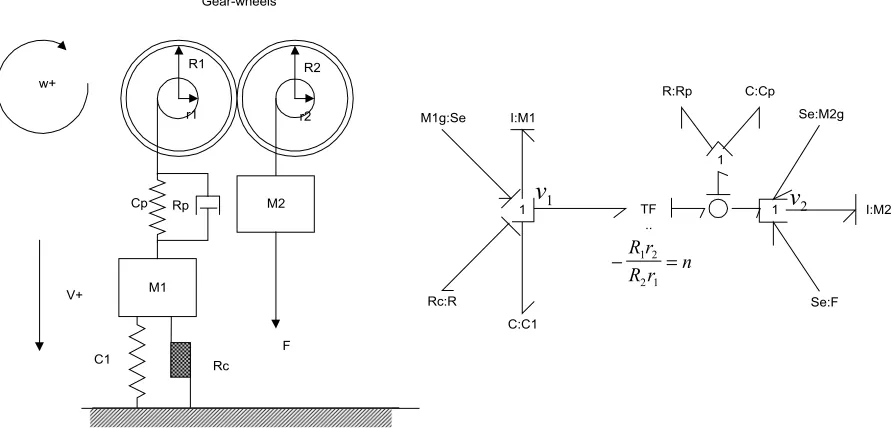
2.5.2 Elimination dependent state by adding spring and damper

In this case the added spring force

F

_Cpand the added damping forces

F

_Rpcontrol the constraints. The forces

F

_Cp

+

F

_Rp control in such a way that the velocity constraints are satisfied. A system can contain several dependent states, for every dependent state that we want to eliminate we must add a spring-damper combination. Every spring that we add causes an extra state variable,

x

_A is the vector of additional state variables. Now the total state

x

_Tvector becomes

[

]

x

_TT

x

x

A T

=

|

∈

χ

,

where x is the original state vector and

χ

_T

= ℜ

4. When the energy of the spring is added, the total energy becomes

H (T xT)=H( ) H (x + A xA), where

HA A CpC T

p Cp (x )= 1x − x

2

1

and whereCp−

1 _{is the vector of spring constants. Now, the control input}

λ

_{of system (2.1)-(2.5) can be}

written as

λ

=

∂

H

∂

+ = − +

x R C R

A A A

Cp A Cp p Cp Cp ( )

& &

x

This controller is equivalent to a PD controller with respect to position xCp, where Cp

−1

is equal with the proportional factor and RCp (vector of damping constants) is equal with the differential factor. The

spring constants Cp should be chosen small enough to obtain a acceptable violation of the velocity

constraint.

Example:

We will eliminate dependent state p2from the Gear-wheel model by means of adding spring and

damper. The Gear wheel model contains only one dependent state. The forces

F

_Cp

+

F

_Rp control in such a way that –nv1+v2 is constrained to zero, where n

R r R r

= − 1 2 2 1

. Figure 3 shows that the dependent state is eliminated.

Gear-wheels

R1 _R2

r1 r2

M1

M2

C1 _Rc F

V+ w+

1 TF

..

C:C1 Rc:R

M1g:Se I:M1

−R r_{R r}1 2 =n 2 1

v

1

1

I:M2 1

Se:M2g

Se:F

v

₂

R:Rp C:Cp

Cp Rp

Figure 3 : Gear-wheels: Parasitic-elements approach used to eliminate the constraint Index 0 system:

When we add a spring and damper to eliminate dependent state p2 the total state vector becomes

[

]

x

_TT

Cp

p

x p

x

=

1 2

∈

χ

& & & & p x p x

Rc n R

M C

nR

M nCp M n R M nR M C n M M p x p x M g

M g F Cp cp cp cp cp p Cp 1 2 2

1 1 2

1 2 1 2 1 2 1 2 1 2 1 1 1

0 0 0

0 1

0 1 0

0 0             = − − − − − −                                     + ₊             . (2.29) Eigenvalues:

The eigenvalues of (2.29) can be calculated by solving the following equation

det(

λ

I

_n

−

Ax

)

=

0

. Where, A= − − − − − −                         Rc n R

M C

nR

M nCp M n R M nR M C n M M cp cp cp cp p 2

1 1 2

1 2 1 2 1 2 1 1 1

0 0 0

0 1

0 1 0

.

When these matrices are substituted and when the numerical values of the Gear-wheel model are substituted the polynomial becomes.

λ

4 ₊₄₀₀

λ

3 _{+40004 5,}

λ

2 ₊₇₀₀

λ

_{+50000 0=}

The roots of this polynomial are,

λ

, ,1 2 = −200 0 5± , i

λ

3 4, = −0 0025 1118, ± , i

Stiffness ratio:

We can calculate the stiffness ratio by means off

S i i

i i

= max Re( ) = =

min Re( ) , .

λ

λ

200

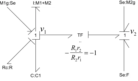
2.5.3 Elimination dependent state by symbolic index reduction

In Figure 4 the inertia with the derivative causality is transferred to the inertia with integral causality and the two masses are replaced by an equivalent element. In the case of this simple example the transformation can be done by hand. For more complex models it is possible to use mathematical software to manipulate equations. In both cases extra manipulation of the equation is needed.

1 TF

..

C:C1 Rc:R

M1g:Se I:M1+M2

− R r = −

R r 1 2 2 1 1

v

₁ 1 Se:M2g Se:F

v

₂

Figure 4 : Gear-wheels: The transfer of dependent storage elements is used to eliminate the constraint Index 0 system:

The general equation is given by

p x

Rc

M M C

M M

p x

M g M g F

n n • •           = − + − +                  + + +     

1 2 1 1 2 1 2

1

1

0

0

. Eigenvalues:

The eigenvalues can be calculated by solving the following equation det(

λ

I_n −Ax)=0.

Where, A= − + − +             Rc

M M C

M M

1 2 1 1 2

1

1

0

.

When these matrices are substituted and when the numerical values of the Gear-wheel model are substituted the polynomial becomes.

λ

2 _{+0 005,}

λ

_{+1 25 0, =}

The roots of this polynomial are,

Stiffness ratio:

We can calculate the stiffness ratio by means off

S i i

i i

= max Re( ) = =

min Re( ) , ,

λ

λ

0 0025 0 0025 1

Because S=1, the system is a non-stiff system.

2.6

summary

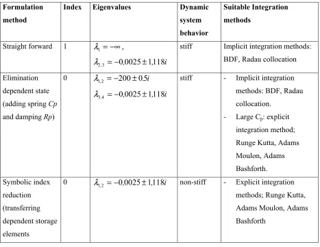
The way the system is formulated determines the eigenvalues and it determines the index of the system and therefore the integration methods that can be used to solve the problem. The Flow chart that is presented in Figure 1 can help the modeler in order to find the needed formulation strategy. The flow chart could be implemented in a Decision Support System (DSS). In this chapter a number of formulations of a constrained system are shown. In Table 1 formulation method, the index, the eigenvalues, the system dynamics and the suitable integration methods are shown.

Table 1 : System dynamics Gear-wheel model Formulation

method

Index Eigenvalues Dynamic

system behavior

Suitable Integration methods

Straight forward 1

λ

_{1 = −∞},

λ

2 3, = −0 0025 1118, ± , i

stiff Implicit integration methods: BDF, Radau collocation Elimination

dependent state (adding spring Cp and damping Rp)

0

λ

_{1 2,} = −200 0 5± . i

λ

3 4, = −0 0025 1118, ± , i

stiff - Implicit integration methods: BDF, Radau collocation.

- Large Cp: explicit

integration method; Runge Kutta, Adams Moulon, Adams Bashforth. Symbolic index

reduction (transferring dependent storage elements

0

λ

_{1 2,} = −0 0025 1118, ± , i non-stiff - Explicit integration

methods; Runge Kutta, Adams Moulon, Adams Bashforth

.

• The bond graph model that is obtained from the gear wheels system has a dependent state. The equation can be formulated as an index 1 or index 2 system. When the index is reduced by means of adding spring and damper the obtained equation has index 0.

• The straightforward approach and elimination of the dependent state by adding spring and damper approach obtain stiff systems that have to be solved by implicit integration methods.

• The elimination of the dependent state by adding spring and damper approach obtains an index-0 system, so it is an ODE. However, because the system is stiff it has to be solved by mean of an implicit integration method.

3

Implicit integration methods

3.1

Introduction

The goal of this chapter is to explain implicit integration methods. Implicit integration methods are stable for index 1 systems and semi explicit index 2 systems when some conditions are satisfied (Ascher, 1998). In chapter 4 we will discuss index reduction by means of feedback linearization and stabilization. In chapter 5 we will compare implicit integration method with the feedback linearization method. Examples of implicit integration methods are Backward Differential Formula (BDF) and Radau collocation (Ascher, 1998) (Petzold, 1982)

3.2

Numerical techniques for implicit integration methods

The important numerical parts of implicit integration methods are: discretization by polynomial basis, the modified Newton iteration and step size control. Discretization is possible by interpolating polynomials with fixed coefficients, variable coefficients or fixed leading coefficients. This choice dominates the computer load. For example, with a variable coefficient strategy the coefficients change when the step size changes and in this case a new Jacobian must be calculated. The calculation of the Jacobian determines the computational border. However, because of the error, due to interpolation, it can be necessary to change the step size to get a stable polynomial. A good alternative for the variable coefficient strategy is the fixed leading coefficient polynomial. With this polynomial only the leading coefficient is adopted when the order changes. The rest of the coefficients remain constant. Every time step, the DAE is solved by Newton iteration. By only calculating the iteration matrix when necessary the computer load becomes less. The accuracy of the modified Newton iteration determines the amount of the drift on the manifold. The step size and order are adapted in such a way that the computer code can solve the DAE while satisfying the tolerance with the minimum computer load.

3.2.1 Polynomial basis

Suppose that a function x( )t is know at time instants t_i for i = 0, 1, .., k, for example x(t_{n i−} )= x_{n i−} . It can be estimated by constructing an interpolating polynomial. For example, the variable coefficient k-order polynomial (Newton form) is given by

x( )t = x_n + −(t t_n)[x x_n, _n−1] (+ −t t_n )(t t− _n−1)[x x_n, _n−1,x_n−2] ...+ . (3.30)

Where

[

]

[

,

,...,

, ]

[

,

,...,

] [

,

,...,

]

x

x

x x

x

x x

x

x

x

x

n n n n n k

n n n k n n n k

n n k

t

t

=

=

−

−

− − − − + − − −

− 1

We can estimate

x

&

( )

t

at time step

t

_nby differentiating this polynomial. In our case

&

( ) [

,

] (

)[

,

,

] ...

x

t

_n

=

x x

_{n n−}1

+

t

_n

−

t

_n−1

x x

_{n n−}1

x

_n−2

+

. (3.31)

The general DAE is given by,

F x x

(

&

, , )

t

=

0

, (3.32)

Substituting (3.31) into (3.32) gives,

F x x

([

_n

,

_n−1

] (

+

t

_n

−

t

_n−1

)[

x x

_n

,

_n−1

,

x

_n−2

] ...,

+

x

_n

, )

t

_n

=

0

.

This is a non-linear equation with respect to

x

_n, its solution gives a new value

x

_n.

Example: First- order BDF

When

x

&

( )

t

_n

=

f

( ,

t

_n

x

_n

)

, the first-order variable coefficient BDF is given by

h

_n

f

( ,

t

_n

x

_n

)

=

x

_n

−

x

_n−1, (3.33)

Multistep equations are generally presented as follows

α

j n j

β

j

j k

n j j

k

h

x

₋

f

= − =

=

∑

∑

0 0

. (3.34)

The coefficients of the first-order BDF are,

k

=

1

,

α

₀

=

1

,

α

₁

= −

1

and

β

₀

=

1

.

Example: Second-order BDF

When

x

&

( )

t

_n

=

f

( ,

t

_n

x

_n

)

, second-order variable coefficient BDF is given by

h t h

h h h h

n n n n n

n n n

n n n

n n n f( ,x )= x −x + ₊ x −x − x −x



 

 

−

−

− − −

− 1

2 1

1 1 2 1

, (3.35)

When the step sizes are taken fixed and equally spaced this equation becomes

h

_n

f

( ,

t

_n

x

_n

)

=

3





x

_n

−

x

_n−

+

x

_n−





2

4

3

1

3

1 2 . (3.36)

When this BDF is written in the general multistep form, (3.34), the coefficients are

k

=

2

,

α

₀

=

1

,

α

1

= −

4 3

/

,

α

2

=

1 3

/

and

β

0

=

2 3

/

.

(3.35) shows that the coefficients depend on the step size and on the previous step sizes. The fixed leading coefficient BDF is given by

h

_n

t

_{n n n n j}

j k

n j

f

( ,

x

)

= −

$

x

+

x

= −

∑

α

0

α

1

. Where the leading coefficient is given by

$

α

0

1

1

= −

=

∑

j

j k

and the rest of the coefficients are constant. So, the polynomial only depends on order and not on step size. This can save Jacobian calculations when this polynomial is used in Newton iterations.

3.2.2 Modified Newton iteration

The following equation has to be solved

F x

(

_nm

)

=

₀

_.

Suppose that in step m,

x

_nm_{is obtained. We would like to derive}

x

n

m+1 _{so that}

F x

(

)

n

m+1

=

₀

_.

The problem will be solved by expanding

F x

(

_nm

)

_{into Taylor's series around the point}

x

nm+1, for

example

0

1 1 1

=

+

≈

+









−

= − +

F x

F x

x

_{x x}

x

x

(

_nm

)

(

)

(

)

nm nm nm

F

nm

∂

∂

.

Solving the last equation for

x

_nm+1_{, so called Newton iteration formula is obtained}

x

x

x

_{x x}

F x

n m n m n m

F

n m + = −

=

−









1 1

∂

∂

(

)

. (3.38)

In this case m is the number of the iteration step. Now we will take the first order fixed coefficient BDF polynomial as an example. The problem to be solved is

F x

(

_n

)

=

x

_n

−

x

_n−1

−

h

_n

f

( ,

t

_n

x

_n

)

=

0

, (3.39)

Substituted in the Newton equation. The iteration formula is given by

x

x

I

f

x

_{x x}

x

x

f

x

nm nm

h

n nm nm

h

n

t

n nm

m m + = − −

=

−





−





−

−

1 1 1

∂

∂

(

( ,

)

, (3.40)

The matrix

(

I−h_n f x

)

_{x x}−₌

nm

∂ ∂

/ 1 is called the iteration matrix. Usually the iteration can be started with

x

_n0

x

_n

1

=

₋ . DAE solvers use more complex strategies like the fixed leading coefficient strategy. In this case the initial guess is done by evaluating the variable coefficient BDF and the Newton iteration is done by a fixed leading coefficient BDF. In this case the BDF polynomial is given by

F x

(

_n

)

$

_n

x

_{n j}

x

f

( ,

x

)

j k

n j

h

n

t

n n

=

−

+

=

= −

∑

α

0

α

1

0

. (3.41)

Where the iteration matrix looks like

$

$

&

G

f

x

f

x

_{x x}

=





+





=

α

n

∂

∂

h

n

∂

∂

n m

0 _{. (3.42)}

3.2.3 Step size control

Because the step size and the order are variable, the non-linear DAE can be solved with a good

accuracy and with relatively less computer load. The order and step size depend on the local truncation error. The order of the next step is chosen in such a way that it is as large as possible and the step size is chosen in such a way that the error estimate satisfies the tolerance.

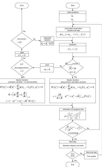
3.2.4 Flow chart

The software code has three iteration loops; the time update loop, the Newton iteration loop and the stepsize minimization loop.

1. The Time update loop:

The Time update loop is done by the main loop, the iteration variable is n. The iteration is updated during the simulation time.

2. The Newton iteration loop:

The iteration variable is m. The iteration is executed every time step n. Before the Newton iteration is started the polynomial is constructed by means of previous calculated states

x

_{n i−} for i = 0, 1, .., k. In order to minimize computer load the iteration matrix (Jacobian) and the LU decomposition will only be evaluated when necessary. The iteration matrix will be evaluated when:

• The iteration fails to converge.

The Newton iteration is considered to converge when

ρ

ρ

1

0 33

1

−

x

nm+

−

x

nm

<

.

ETOL

Where ETOL is the user tolerance,

ρ

is an indication of the rate of convergence of the iteration, which can be estimated by

ρ

= −

−

   

   

+

x x

x x

n m

n m n n

m

1 1 0

1

.

The norm is a root mean square norm and

ETOL

=

RTOL

x

+

ATOL

.

• When the new step size or order largely differ from the previous ones. In this case

α

_n0

≠

α

$

_n0. Where the true leading coefficient is

α

0

1 1

= −

−

₋

=

∑

t

h

n

t

n n j

k

,

$

α

0

1

1

= −

=

∑

j

j k

.

To decide if a new iteration matrix must be calculated the eigenvalues (

λ

) of

G

are estimated. When c a new Jacobian must be calculated. In DAE solver DASSL

µ

=

0 25

,

. When some previous evaluated Jacobian

G

$

_previous is used, the variable c is added to the Newton iteration formula. The iteration formula becomes

x

_nm

x

G

F x

nm

c

previou nm

+1

=

−

$

−1

(

)

_and

the condition

B

= −

I

c

G

$

−

G

<

previous1

1

must be satisfied. When ODE

x

&

=

Ax

will be

calculated the eigenvalues are

λ

. When these eigenvalues are substituted in

B

the

eigenvalues of

B

are

λ

. Because the eigenvalues of

G

can't be calculated for a DAE, they are taken in such a way that the eigenvalues of

B

are minimized in the left half of the complex half plane. This leads to c=2

α α α

$/ ( + $) and the estimated eigenvalues of

G

are

λ

=

(

α α

$

−

) / (

α α

+

$

)

.

• A certain number of steps have passed.

When the iteration number of the Newton iteration loop is bigger then 4 and the iteration doesn't converge a new iteration matrix will be calculated.

3. Step size minimization loop:

The iteration variable is l. The iteration is executed when the Newton iteration fails to converge after two LU decompositions. In this case the step size is made smaller by a factor 0,25.

prediction

x(tn)=xn0

polynomial construction, variable time step

x(tn i−)=xn i− i=1,....,k+1

Start initial conditions x x 0 0 & Newton iteration: using previous calculated Jacobian

F x( n ) $ x x f( ,x )

m n n m j j k

n j n n n m

h t

= − + =

= −

∑

α0 α

1

0

c n c

m n m n m = + + = − −

2$ 1 1

$ $ ( )

α

α α x x GpreviousF x Newton iteration:

evaluation Jacobian, LU decomposition

F x( n ) $ x x f( ,x )

m n n m j j k

n j n n n m

h t

= − + =

= −

∑

α0 α

1

0

c n c

m n m

n m

=_{1 x} +1=_x − _{G F x$}−1 _{( )}

$ $

&

G f

x f x _{x x}

=_ + _ = α ∂ ∂ ∂ ∂

n hn

n m 0 No Yes adapatatio stepsize

h_nl h

n l

= −1_{. ,0 25}

Gpreviousexists ?

λ <µ

< m 4 No LU decompositions >2 Yes iterations >10 No Error Yes ρ ρ 1 0 33 1

− x + −x < ETOL n m n m .

estimation convergence rate

ρ= −

−

 

x_xn+ _xx _

m n m n n m 1 1 0 1 Next step

Selection stepsize and order

End time? End No No Yes Yes

Next time step

Time update reset

m:=0

reset

LU :=0

3.3

Summary

4

Index reduction, a control approach

4.1

Introduction

The topic of this study is the solution of the following general model equations that describe nonlinear constrained systems in the form of a control problem

& (

x J x

x x G x G x f G x u

= C + + C,R R + C,U

)

∂

H( ) ( ) ( ) ( ) ,

∂

λ

(4.43)

Φ

( )_{x G x}T( ) H( ) x x

= =0

∂

∂

. (4.44)

e G x

x x G x u R _{= −(} C,R_{( ))}T

∂

H_{( )+} R,U_{( ) ,}

∂

(4.45)

Ω

(_{f e x}R, R, )_{=0. (4.46)}

These equations are introduced in chapter 2. The control law

λ

must be developed in such a way that (4.44) remains close to the desired trajectory

Φ

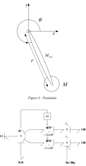
desired( )x =0. This is called control of motion (Slotine,

1991). In this subchapter we will investigate the available nonlinear control and stabilization techniques in order to find a suitable method to control this problem. We want the method to be straight forward and suitable for the solution of complex systems. The control law will be evaluated with respect to the following characteristics: stability, accuracy, robustness, cost. The stability of motion will be investigated by means of the Lyapunov stability theory. The proposed control law and stability investigation will be explained by means of a planar pendulum. This is a relatively small-constrained nonlinear system, which can be solved analytically too.

4.2

Non-linear control

There is no general method for designing nonlinear controllers (Slotine,1991). In this section we give a short description of the available methods. We will select the methods that are suitable to control the described nonlinear constrained systems.

Trial and error:

Feedback linearization:

The basic idea is to first transform a nonlinear system into a linear system and then use linear design techniques to design a controller. This method requires full state measurement. The method doesn't guarantee robustness in the case of parameter uncertainty or disturbance.

Robust control:

In robust nonlinear control (sliding mode control) the controller designed is based on both the nominal model and some characterization of the model uncertainties (for example unknown load masses).

Adaptive control:

Adaptive control design can be applied to systems with known dynamic structure, but unknown constant or relatively slowly varying parameters.

Gain scheduling:

The idea is to select a number of operating points, which cover the range of the system operation. At each point the designer makes a linear, time invariant approximation of the plant and designs a linear controller for this linearized plant.

A Selection of a suitable method to control the constrained nonlinear system (4.43)-(4.46) can be made as follows:

4.3

Control design

4.3.1 Feedback linearization

The basic idea of feedback linearization is to cancel the nonlinearities in a nonlinear system so that the closed loop dynamics is a linear form (Slotine,1991). We can generate a linear input-output relation by means of differentiation of the output and then formulate a controller by using linear control. This is called the input-output linearization approach. The relation between the output

Φ

(x) and the input

λ

of system (4.43)-(4.46) can also be found by repeated differentiation of the output. In this case the violation of the constraint

Φ

(x) is called output of the system. If we need to differentiate the output of the system r times in order to generate a unique explicit relationship between the output

Φ

(x) and the input

λ

, the system is said to have relative degree r. The relative degree is equal with the index of a system, so we can use the same definition. The index of a system is equal to the number of times we need to differentiate the output of the system in order to obtain a unique solution, the definition is given in section 2.3. If we differentiate the output of the concerned system (4.44), the following equation is obtained

&

( )

( )

&

Φ

x

x

x

x

=

∂Φ

=

∂

T

0

,

substitution of equation (4.43) gives

&( ) ( ) ,

Φ

x

Φ

x

x J x x x G x G x f G x u

=

∂

_ + + + _ =

∂

∂

∂

λ

T

C C R R C,U

( ) H( ) ( ) ( ) ( ) 0.

Suppose that the dimension of the generalized state vector x is k and the dimension of the Lagrange multiplier

λ

is n. As n<k, we speak of an underactuated system. Solving the previous equation for

λ

gives

λ

∂

∂

∂

∂

∂

∂

∂

∂

∂

∂

= −_ _ _ + + _

−

Φ

( )

Φ

( )

Φ

( )

Φ

( )

. ,

x x G x

x

x J x x x

x

x G x f

x

x G x u

T T

C

T

C R R

T C,U

( ) ( ) H( ) ( ) ( )

1

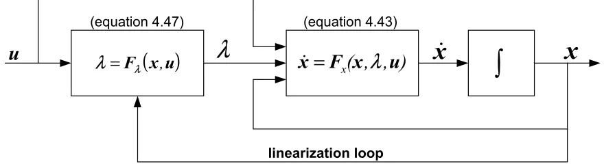
(4.47) Figure 6 shows the block diagram of the closed-loop system (4.43) controlled by control law (4.47).

( )

λ

=

F x u

λ

,

u

x

linearization loop

λ

x F x

&

=

, ,

u

x

(

λ

)

x

&

∫

(equation 4.43) (equation 4.47)

4.3.2 Nonlinear controller

In this study constraints at the velocity level are considered. In this section we will take a closer look at the velocity constraints and we will construct the nonlinear controller equivalent with the feedback linearization.

In order to be able to investigate the constraints at the velocity constraint, we consider a mechanical system described by position state vector q. When the constraints are velocities

q

&

described by

( )

G q qT

& this will lead to the following constraint equation

( )

( ) ( )

Φ

p q

,

=

G q M

T −

q p

=

p1

0

(4.48)

and the following Hamiltonian constraint equation

( )

( ) ( )

Φ

p q

G q

p q

p

,

=

T

∂

H

,

=

∂

0

. ` (4.49)

Where p represents the momentum of mass Mp(q). This equation is the equivalent with (4.44)

concerning the velocity constraint. Now we will apply the feedback linearization control law (4.47). First (4.48) is differentiated

( )

(

( ) ( )

)

( ) ( )

(

)

(

( ) ( )

)

& ,

& &

Φ

p q G q M q p

G q M q p

q q

G q M q p

p p = = + = − − −

∂

∂

∂

∂

∂

∂

T p T p T p t 1 1 1

( ) ( )

(

)

( )

( ) ( )

∂

∂

G q M q p