R E S E A R C H
Open Access
Coded unicast downstream traffic in a wireless
network: analysis and WiFi implementation
Asaf Cohen
*, Erez Biton, Joseph Kampeas and Omer Gurewitz
Abstract
In this article, we design, analyze and implement a network coding based scheme for the problem of transmitting multiple unicast streams from a single access point to multiple receivers. In particular, we consider the scenario in which an access point has access to infinite streams of data to be distributed to their intended receivers. After each time slot, the access point receives acknowledgments on previous transmissions. Based on the acknowledgements, it decides on the structure of a coded or uncoded packet to be broadcast to all receivers in the next slot. The goal of the access point is to maximize the cumulative throughput or discounted cumulative throughput in the system. We first rigorously model the relevant coding problem and the information available to the access point and the receivers. We then formulate the problem using a Markov decision process with an infinite horizon, analyze the value function under the uncoded and coded policies and, despite the exponential number of states, devise greedy and
semi-greedy policies with a running time which is polynomial with high probability. We then analyze the two users case in more detail and show the optimality of the semi-greedy policy in that case. Finally, we describe a simple implementation of the suggested conceptswithina WiFi open-source driver. The implementation performs the network coding such that the enhanced WiFi architecture is transparent above the MAC layer.
1 Introduction
The inherent broadcast nature of the wireless medium, which allows each transmission to be heard by all users simultaneously, makes network coding techniques per-tinent. In such techniques, nodes do not necessarily forward incoming packets. Rather, they can transmit a manipulation (usually a linear combination [1]) of their incoming data. However, in order for such a combina-tion to be valuable to multiple users, each such user needs to possess different piece of the information encoded into the combined packet. Accordingly, one of the key challenges in network coding techniques is to decide which packets to manipulate in each transmission. While efficient algorithms answer this challenge in the multi-cast setting [2], the problem of multiple unimulti-cast remains open [3].
On the down side, the wireless medium characteristics make wireless transmissions susceptible to losses due to noise and interference (i.e., low SNR and SINR). In order
*Correspondence: [email protected]
Department of Communication Systems Engineering, Ben-Gurion University of the Negev, Beer-Sheva, 84105, Israel
to cope with packet loss in MAC layer, conventional wire-less protocols rely on retransmissions (e.g., WiFi, [4]). In such protocols, each packet has to be acknowledged by the intended receiver. Packets which are not acknowl-edged are retransmitted over and over again until they are received successfully by the receiver, or until dropped by the sender.
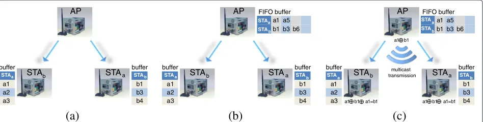
Typical last mile wireless Internet access architecture comprises a gateway, e.g., an access point (AP) or a Base Station (BS), to which all clients are wirelessly connected (e.g., WiFi, WiMAX, LTE). In such architecture, all traf-fic to and from the wired Internet must pass through the gateway via the wireless medium. Accordingly, all trans-missions by the gateway are potentially heard by all clients associated with this gateway. In this article, we utilize these aforementioned wireless properties of channel, pro-tocol and last mile architecture and suggest coded wireless retransmissions for downstream traffic. In particular, we suggest a novel scheme which is based on Markov decision process (MDP [5-7]), that combines multiple MAC layer retransmissions which are intended to different receivers, into a single packet transmission.
1.1 Main contributions
Our contributions are thus as follows. First, we suggest an ongoing process in which the AP (or gateway) alter-nates between transmitting uncoded and coded packets. Receivers acknowledge packets they have received suc-cessfully and in addition provide feedbacks to the AP regarding packets they overheard which were not meant for them. Based on these feedbacks the AP chooses which retransmitted packets (if any) should be coded in each retransmission. Our model is inherently not multicast—
each receiver has a different stream as its demand. More-over, we assume aninfinite horizonmodel, where there is no point in time in which all demands are met and the sys-tem reaches a terminating step. Packets arrive at the AP continuously, and only the current packets for each user are available for coding. Based on this model, we are able to analytically solve throughput problems. We believe that these two aspects of our model are of key importance, since this is the typical use of most wireless Internet access networks.
Second, we show that the aforementioned continuous transmission process can be modeled as a discrete time stochastic process, in which at each state the next state is determined solely based on the AP decision which packet to transmit next (i.e., which coded or un-coded pack-ets should comprise the next transmission) and based on the channel state of each and every receiver which deter-mines which nodes receive the next transmission. We suggest an APpolicywhich is based on MDP theory, in which the reward attained in each iteration corresponds to the number of successful packets received in each transmission.
Third, we leverage this continuous, infinite time stochastic model, to compute stationary behavior, which in turn allows us to define convergence, calculate the resulting asymptotic performance efficiently (using only a set of linear equations), and assess the benefit in coding directly and analytically. Specifically, we give the matrix equation that computes the cumulative expected reward (equivalent to the system throughput when a unit reward is given to decoding of one packet) for any state in the system given the transition probabilities and the reward vector. This enables us to directly compute the perfor-mance ofanycoded or un-coded strategy. For the two user case, we indeed give a few possible strategies and compute the resulting performance.
Fourth, we show that in order to reach an optimal decision, the AP needs to consider all possible future states of the system, channel states of all users and all possible actions and outcomes. This procedure certainly cannot scale to large number of users. Accordingly, we suggest a greedy approach in which at each transmis-sion the AP tries to maximize the instantaneous reward received for each transmission (as opposed to maximizing
an expected or discounted reward, which takes into account the expected rewards at future states). We fur-ther suggest an enhancement to the greedy approach, termed semi-greedy approach, which takes some con-cern into the future, without adding significant complexity to the greedy approach. In the semi-greedy approach, we also suggest a direct analysis for the simple case of two receivers, which besides the analysis of this simple case, also provides some insight into much larger sce-narios. We evaluate both schemes via an extensive set of simulations, which show that our approach attains high gain over the traditional un-coded transmissions while maintaining long time fairness. Moreover, we show that the semi-greedy approach exploits the multi-user diversity in the system, putting more emphasis on serv-ing the users with the best channels conditions at any given time.
Finally, we implement our scheme on a WLAN topol-ogy in which a single AP transmits unicast traffic to two receivers. We show that the suggested scheme can be eas-ily implemented over a typical 802.11 card, with some modifications to the wireless driver. To the best of our knowledge, this is the first implementation of these con-ceptswithin the WiFi driver, and transparently from the upper layers. We further show that at least for this simple case, the experimental gain agrees with the one predicted by our analytical model.
1.2 Related study
At the basis of our study stands the already well under-stood concepts of network coding[1]. In this pioneering study, intermediate nodes in the network perform cod-ing operation on the data in order to achieve certain rate goals. Indeed, it was shown that network coding can improve the network throughput significantly, and achieve the optimal performance in the multicast sce-nario. The theory of network coding includes linear [8,9] as well as non-linear coding techniques. In this article, we focus on coherent linear network coding.
network coding was first introduced in [11,12] as COPE. While decentralized, this groundbreaking work was not tailored to the multiple unicast with one sender scenario we consider in this article. A polynomial time central-ized algorithm, yet with guarantees only for the multicast scenario, was given in [2].
In [13], loss aware coding in wireless multi-hop net-works was considered. Therein, having knowledge of the packets available at each users, the sender is trying to come up with a sequence of transmissions to satisfy as many users as possible. Thus, the model given in [13] is not the Markovian model we consider in this study, and is of finite horizonnature, i.e., where the set of packets to be transmitted is finite and known in advance to the sender, compared to the infinite sequences of data per user we consider here. Note, however, that the assumption that the sender is omniscient, knowing which packets received where, is similar to our setting, and many related studies [14-17].
Also related is the recent study by Sorour and Valaee [18]. Therein, a fixed set of packets is transmitted to all users. Then, after acknowledgments are received, the sys-tem computes which coded packets to send in order to satisfy the demands. A sequence of coded retransmissions is constructed, sent, and only when all users reconstruct all their intended packets the system continues to the next set of packets. Again, this is fundamentally differ-ent from theinfinite horizonmodel we consider herein. In a sense, the model described in our study allows for coding across MBS frames (using the notation of [18]), whereas [18] allows coding only within an MBS frame. Moreover, the scheme in [18] is adapted to the case whereall loss probabilities are equal. The successive stud-ies in [19-21] also consider the finite horizon model, yet contribute significantly to our knowledge in terms of min-imizing delay [19,20] or maxmin-imizing coding opportunities [21].
Studies on opportunistic coding for the finite horizon broadcast case, where users are interested in all pack-ets, and the sender has a fixed set of packets to send
also appeared in [15,16]. Nevertheless, a key difference compared to the model we define herein is in the mul-ticast demand structure—eventually all users demand all the information available. While this demand structure is well-understood [1,8,9], the capacity region in the general source sink setting [22], as well as the multi-ple unicast setting [3], remains unsolved. In the context of the setting discussed in this article, the index coding problem [17], which also considers only a single sender with multiple receivers (having side information), is also unsolved in general. Note that index coding is, in gen-eral, over noiseless channels, and does not include the dynamic, error-prone and infinite time setting we con-sider herein.
In [23], the authors considered a similar star topology, with one server supporting several clients (receivers). The demand structure in [23] is more general compared to the previously discussed studies [14-16], that is, not necessarily all users require all information. However, the model in [23] is different than the one suggested in this article. First, it is a finite horizon model, where all data is available at the server(in advance) for coding. In the model discussed herein, only the packets intended for current transmission (or retransmission) are available at the server for coding. In many streaming applica-tions, this is usually the case, and the server cannot code “future” packets as these, usually, are not available at the time of transmission. The model in [23] also assumes user can buffer all packets, even those who cannot be decoded immediately, requiring working over a large finite alphabet. Moreover, in this case, optimally deciding which coded packet to send is prohibitively complex. For this reason, coding in [23] is done over “classes” of users, and these classes are pre-defined and fixed for the entire transmission. Random linear network coding was used, where coding is only across classes of files. This converted the problem to multiple-multicast sessions (that is, a user is required to decode all files within its class in order to retrieve its own file). Finally, the main figure of merit therein was thedelay. Indeed, a rule of thumb that arose from this work was to avoid coding across files (users, in our model), and code mainly over packets within the same file. The results under our model will be significantly dif-ferent, suggesting it is strictly better to code across users, even though it is a multiple unicast scenario, as long as the subsets of users sought for in the opportunistic coding process are not too large, hence do not create a significant computational burden.
In [14], the authors considered in more detail the spe-cific case of coded retransmissions. That is, given the knowledge of which packets were not received by their intended users, but overheard by others, the authors sug-gest a MDP approach to identify good coding strategies. However, similar to [15,16], all receivers are interested in all packets. In the context of the underlying MDP, note that since [14] assumes a fixed, finite set of packets to be sent to all users, there is a terminating state for the chain, from which the optimal policy can be calculated using backward recursion. However, stating the analytical solution explicitly is not an easy task.
of work on network error correction, e.g., [25-27], and noncoherent network coding [28]. Yet, the majority of these studies focus on general network topology on the one hand and specific multicast demand structure on the other.
On the practical side, several studies implemented net-work coding concepts on real netnet-works. We focus here only on works whose implementation isbelowthe appli-cation layer (i.e., excluding network-coded content dis-tribution and related studies). A pioneering work in this context is the already discussed [12]. The COPE header in this work resides between the routing and the MAC headers. The implementation runs on a 802.11a network as a user space daemon, that is, it sends and receives raw 802.11 frames. Random linear network coding on the iPhone was studied in [29], though, again, the implemen-tation is on top of the WiFi driver, and not within it. Using Nokia mobile devices was suggested in [30]. In [31], the authors considered a chain topology, and gave numerical evaluation of the suggested iCORE scheme. Still, iCORE is a user space daeamon, whichusesWiFi, but does not alter it. In this article, the implementation waswithinthe WiFi driver, rendering the coding procedure transparent to all above layers.
2 System model
We first define the system model we use. We consider a downlink wireless model, with one serving access-point/ base-station (sender) and K users/stations (receivers). At the sender, we assume an infinite stream of packets
for each user. That is, the stream of packets Pki∞
i=1 is
intended to the kth user. Thus, our demand structure is that of multiple unicast sessions, with one common sender. At the receiver, we assume packets transmitted to other users are cached (if heard), even though those packets are not intended to itself.
We consider a synchronized system, where the time is divided to discrete slots. At each slot, the sender can send one packet. Our channel model is as follows. At each slot, the packet sent is received at receiver k with probability pk, independently of the other receivers and
of the packets received previously (memoryless indepen-dent users). However, when a receiver correctly receives a packet, it broadcasts an acknowledgment, together with its user indexi. We assume this acknowledgement is cor-rectly received by both the sender and all other receivers. We comment on the possibilities to relax this assumption in Section 4.5.
At each time instant, the sender chooses a packet to send, according to its assessment of thestatethe system is in. However, since the state definition and evolution is intertwined with the coding strategy used, we first describe the possible coding strategies.
2.1 Network coding strategies
Each time a packet is sent, the sender can either choose a packet to send to a single user, or code together a few packets. We assume the standard coherent linear network coding model, e.g., [8,32]. The stream intended to each user can be represented as an infinite stream of bits. This stream is split into packets, each represented asm sym-bols in a finite field Fq, for a total of mlogq bits per packet.
In an uncoded packet sent by the access point, sim-ply a packet intended to a single user is sent. In a coded packet, the access point sends a linear combination over Fq of packets. In our model, the access point does not code over packets intended to the same receiver, only across packets intended to different receivers. That is, a sent packet has the formX=Kj=1ajXj, whereXjis the packet
currently intended to user j and {aj}Kj=1 ∈ FK
q are the coding coefficients. Note that an uncoded packet can be treated as a coded one, with all coefficients but one equal zero.
Since the access point keeps track of the current packet requested by a receiver, packets within a coded packet can be labeled using the receiver ID alone. To keep track of the linear combination of the uncoded packets contained in a coded one, a coefficient for each uncoded packet (i.e., for each receiver) is sent in the header of each coded packet. Similarly to prior work on network coding, we assume that the packet payload is sufficiently large compared to the header. This renders the overhead of the header negligible. Clearly, the ability of a user to decode its intended packet depends on its available information. In the gen-eral network coding setting, a receiver keeps track of the coded packets it received. The coefficient vectors of these coded packets are stored in a matrix. Once it is full rank, the data can be decoded. In this study, however, we con-sider a different setting, where a user only keeps track of uncoded packets it received, or packets it decodedat that time instant, and disregards coded packets from which it cannotinstantaneouslydecode original packets. For this reason, it is possible to limit the fieldFqto be binary, and
avoid the complexity burden of larger fields. This can be compared to network coding models where the field size must scale with the number of users (e.g., linear [2]). Note that the extension to a model where a user keeps track of coded packets and the associated vectors of coefficients, even if these cannot lead to decoding at the same time slot, is conceptually simple, but practically does not scale to a large amount of multicast sessions, as the dimension of thestate spacewill be prohibitively large.
2.2 State model
on we assume each receiver hask−1 buffers for storing at most one packet for each other receiver in the system. Namely, when a receiver overhears a packet intended to a different receiver,or it can decodea packet intended to a different user, it is able to store one such packet. This gives rise to our state model, which is at the basis of the system we propose. The state of the system at each time instanttis aK×KmatrixS. The state matrix is initial-ized to the all-zeros matrix. When packets are received at the users, the state matrix updates as follows: fork =k,
Sk,k = 1 if packet intended for user k was heard by
userkandSk,k = 0 otherwise. However, when a packet
intended for userkis received by that user,Sk,k remains
0. This is since we assume once a packet is received at the intended receiver, it immediately sends an acknowledge-ment, together with his indexa. The sender thus knows that the packet was received, and that this user is now awaitingits next packet. Hence,Sk,kremains 0. Moreover,
since the acknowledgement was received by all other users as well, the users which buffered this packet can discard it, as it will no longer be used in coded packets. As a result, if a receiverk acknowledges receiving a packet, all other users who kept it discard it and we setSk,k =0 for allk.
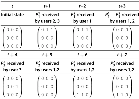
An example of the evolution of the state for three users is given in Table 1. Note that since there are three users, the state is represented by a 3×3 matrix. Additionally, the table only depicts the evolution of the states, assuming the actions (packets sent) as well as their results (where were the packets received) are as given in the table.
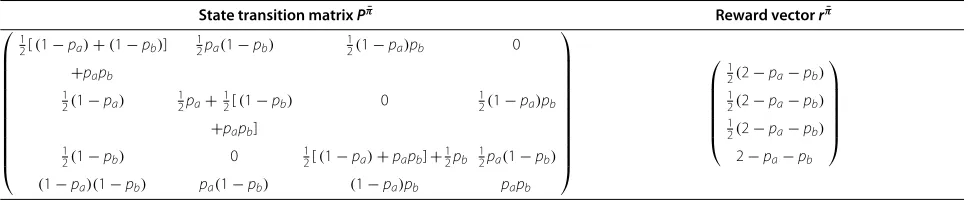
Clearly, it is also important to depict the actual state transition matrix, given the memoryless probabilities of packet losses. For the sake of clarity, we depict here only the two-users case. Table 2 includes the possible states. Table 3 includes the state transition matrix and reward vector withuncoded transmissions and equal loss prob-abilitiesp. In this policy, marked byπ, the sender sends
Table 1 Evolution of the state for three receivers
t t+1 t+2 t+3 Initial state P1
1received P21received P11+P21received
by users 2, 3 by user 1 by users 1, 2
⎛ ⎜ ⎜ ⎝
0 0 0
0 0 0
0 0 0
⎞ ⎟ ⎟ ⎠ ⎛ ⎜ ⎜ ⎝
0 1 1
0 0 0
0 0 0
⎞ ⎟ ⎟ ⎠ ⎛ ⎜ ⎜ ⎝
0 1 1
1 0 0
0 0 0
⎞ ⎟ ⎟ ⎠ ⎛ ⎜ ⎜ ⎝
0 0 0
0 0 0
0 0 0
⎞ ⎟ ⎟ ⎠
t+4 t+5 t+6 t+7
P2
2received P22received P31received P23received
by user 3 by users 1,2 by users 1,2 by users 1,2
⎛ ⎜ ⎜ ⎝
0 0 0
0 0 1
0 0 0
⎞ ⎟ ⎟ ⎠ ⎛ ⎜ ⎜ ⎝
0 0 0
0 0 0
0 0 0
⎞ ⎟ ⎟ ⎠ ⎛ ⎜ ⎜ ⎝
0 0 0
0 0 0
1 1 0
⎞ ⎟ ⎟ ⎠ ⎛ ⎜ ⎜ ⎝
0 0 0
0 0 0
1 1 0
⎞ ⎟ ⎟ ⎠
Table 2 State space for the two users case (coded and uncoded)
S1 S2 S3 S4
⎛
⎝0 0
0 0
⎞ ⎠
⎛
⎝0 1
0 0
⎞ ⎠
⎛
⎝0 0
1 0
⎞ ⎠
⎛
⎝0 1
1 0
⎞ ⎠
a packet at random, either to the first user or to the sec-ond, with equal probability. Table 4 includes the coded
scenario, with unequal loss probabilitiespaandpb. In this
policy, marked byπ¯, since there are only two users, and users do not save coded packets, the only coding oppor-tunity is when each user has a packet intended to the other (stateS4). In any other state, packet is sent at ran-dom, either to the first user or to the second, with equal probability.
3 Markov decision processes—preliminaries
In this section, we give a brief description of the decision process model we use, the required notation and known methods and results which are relevant to this study and will be used throughout. A detailed, more thorough review of decision processes and reinforcement learning can be found in [5-7].
We consider a discrete time time-axis,T = 0, 1, 2,. . .. Note that we do not consider a fixed time N denoting an end state, and rather consider an infinite time model. We assume the system is defined on a finite state space
S. As mentioned, in our model these states represent the knowledge at the terminals. At each time instantt, the sender takes an actionat(st), wherestis the current state.
The actions belong to a predefined setA. Without loss of generality,Aincludes all possible actions from all states at all times. As an example, actions may include sending uncoded messages, sending coded messages, etc.
We assume a Markovian state transition structure, that is
pt(st+1=s|st,at)
=pt(st+1=s|st,at,st−1,at−1,. . .,s0,a0),
and further assume stationarity, i.e.,pt(st+1=s|st,at)=
p(s|s,a). We assume the policies which govern the actions taken are Markovian, that is,at=πt(st). Hence, the policy
depends only on the current state. It is also beneficial to assume that the policies are stationary, that is,at=π(st).
Table 3 State transitions for the two users case: uncoded transmission(pa=pb=p)
State transition matrixPπ Reward vectorrπ
⎛ ⎜ ⎜ ⎜ ⎜ ⎜ ⎝
p2+(1−p) 1
2p(1−p) 12p(1−p) 0
1
2(1−p) p+12(1−p)2 0 12p(1−p)
1
2(1−p) 0 p+12(1−p)2 12p(1−p)
0 12(1−p) 12(1−p) p
⎞ ⎟ ⎟ ⎟ ⎟ ⎟ ⎠ ⎛ ⎜ ⎜ ⎜ ⎜ ⎜ ⎝
1−p
1−p
1−p
1−p
⎞ ⎟ ⎟ ⎟ ⎟ ⎟ ⎠
describe the asymptotic system behavior, and gain insight on the benefits of different strategies.
With each current state, action and next state, we asso-ciate a rewardr(s,a,s). The reward associated with the states and action might reflect both the benefit of transi-tion (e.g., decoding packets) and the cost in the specific action (e.g., the computational complexity in construct-ing a coded message). Again, the reward model does not depend on time, but can be stochastic, that is, with some probability packets are decoded and the reward is high and with some probability there is a loss or a decoding failure. Moreover, we will be interested in thediscounted rewardin the asymptotic regime, that is
Vγπ(s)=Eπ
∞
t=0
γtr(st,at,st+1)|s0=s
,
whereπ is the policy used andsis the initial state. 0 < γ < 1 is thediscount factor. It determines the amount of memory in the performance measure. That is, forγ → 0, the value per state is mainly affected by the current reward, and does not take into account future transi-tions, whileγ → 1 weights almost identically the entire sequence. Vπ
γ(s) is thus the asymptotic cumulative dis-counted reward of the system. Clearly, our goals are to computeVπ
γ(s)for a given policy and find the optimal pol-icy in terms of minimizingVπ
γ(s). For the infinite horizon, stationary model we discuss in this article, these two goals are within reach. This way, it will be possible to, for exam-ple, understand when coding should take place and when uncoded packets are optimal and what is the resulting throughput in the system for each scheme.
The main two results for MDP in the stationary regime are the following.
Theorem 1 (e.g., [5,6]).Let π be a stationary policy. Then, the asymptotic discounted reward Vπ
γ is the unique solution to the following set of linear equations:
Vγπ(s)=
s∈S
p(s|s,π(s))
r(s,π(s),s)+γVγπ(s)
, s∈S.
(1)
To facilitate a vector representation, we denote byVπ γ ∈ R|S|the vector of values achieved by the policyπ, byPπ the state transition matrix under π, that is Pπ(s|s) = p(s|s,π(s)), and byrπthe expected reward
rπ(s)=
s∈S
p(s|s,π(s))r(s,π(s),s).
Under this notation, we have
Vγπ =I−γPπ−1rπ, (2)
that is, in the stationary asymptotic regime, the total rewards achieved by each policy are easily calculated using a linear system. In our setting, (2) will be used to assess the value of a given policy, and compare it to other policies. For example, assess the value achieved by a certain coding policy compared to an uncoded one. However, in certain cases, it is interesting to compute the value function of the optimal policy directly, as well as the optimal policy itself. For this, the following results come in handy. In this case, however, we assume deterministic policiesb. Define the following operator fromR|S|toR|S|,Tγ∗:(Tγ∗V)(s)= maxa∈As∈Sp(s|s,a)
r(s,a,s)+γV(s).
Theorem 2 (e.g., [5,6]).For any initial value function V0, we have
Table 4 State transitions for the two user case: coded transmission
State transition matrixPπ¯ Reward vectorrπ¯
⎛ ⎜ ⎜ ⎜ ⎜ ⎜ ⎜ ⎜ ⎜ ⎜ ⎜ ⎜ ⎝ 1
2[(1−pa)+(1−pb)] 12pa(1−pb) 12(1−pa)pb 0
+papb
1
2(1−pa) 12pa+12[(1−pb) 0 12(1−pa)pb
+papb]
1
2(1−pb) 0 21[(1−pa)+papb]+12pb 12pa(1−pb)
(1−pa)(1−pb) pa(1−pb) (1−pa)pb papb
⎞ ⎟ ⎟ ⎟ ⎟ ⎟ ⎟ ⎟ ⎟ ⎟ ⎟ ⎟ ⎠ ⎛ ⎜ ⎜ ⎜ ⎜ ⎜ ⎝ 1
2(2−pa−pb)
1
2(2−pa−pb)
1
2(2−pa−pb) 2−pa−pb
Table 5 Values ofVγπandVγπ¯ with a discountγ =0.5 and different values of packet loss probabilityp
Packet loss and policy S1 S2 S3 S4
p=0.1, uncoded 1.8 1.8 1.8 1.8
p=0.1, coded 1.80231 1.82803 1.82803 2.708
p=0.5, uncoded 1 1 1 1
p=0.5, coded 1.01111 1.05556 1.055556 1.58889
1. Value iteration: IfVn+1=Tγ∗Vn, thenVn→V∗, the
value function under the optimal policy. 2. Any policyπ∗which satisfiesπ∗(s)=
argmaxa∈As∈Sp(s|s,a)r(s,a,s)+γV∗(s)is
an optimal policy.
3. Policy iteration: Assumeπ¯ is defined according to ¯
π (s)=
argmaxa∈As∈Sp(s|s,a)r(s,a,s)+γVπfor
some policyπ. ThenVπ¯ ≥Vπwith equality iffπis an optimal policy.
4 A Markov decision process based approach
As mentioned in Section 3, in the stationary model under discounted reward, suggested policies can be evaluated analytically, with a closed form solution. We first give here a basic 2-users example. An access point has two streams of packets, one for each of the two users. The four possible states are the ones given in Table 2. Pack-ets are received at each receiver with probability 1− p, independently of the other. Each time a receiver decodes
its intended packet, a reward of 1 is received. The transi-tion probability matrices and reward vectors were given in Tables 3 and 4. We can now findVγπ andVγπ¯ directly according to (2). The solutions for different values of the packet loss probabilitypare given in Table 5. Note that the value function in the coded case is higher than that of the uncoded case for all statesSi,i ∈ 1,. . ., 4. Clearly, while
the value function is constant for all states in the uncoded policy, in the coded policy it is significantly higher for
S4.
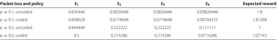
To conclude this example, we calculate the stationary distributions associated with each of the two policies— the uncoded and the coded one. That is, letvπ
s and vπs¯
be the stationary distributions of the uncoded and coded policies, respectively. We have
vπs =(v1,. . .,v|S|): (v1,. . .,v|S|)TPπ =(v1,. . .,v|S|)T. (3)
vπ¯
s is calculated in a similar fashion. The total expected
discounted reward is thusRπ=(vπ
s)TVγπfor the uncoded case and similarlyRπ¯ for the coded one. The results for different values ofpare given in Table 6. Note that since we considercumulative discounted reward, the total sys-tem throughput under a policyπ,in packets delivered per time slot, is(1−γ )Rπ.
The benefit in the coded policy is clear, and it grows larger as the packet loss probability increases. This will also be clear in the simulations. Note, however, that the system of equations is of dimension |S|. For this reason, we include more efficient methods in the next sub-sections.
4.1 A greedy algorithm
The model discussed thus far, allowed us to analytically compute the reward associated with each state and action pair, as well as the expected discounted reward for a given policy. Moreover, using Theorem 2, it is possible to com-pute the optimal policy. However, in practical situations, the equations given in Theorem 2 are computationally intractable. Note that forKusers, the state matrix is of size
K×K, with theKdiagonal values fixed at 0. Thus, the state space is of size 2K(K−1), making it practically impossible to list all states, a fortiori compute all entries of the state tran-sition matrix analytically. Using a reinforcement learning approach, such asQ-learning, would also be intractable as is with such a state space. The reason is, at the basis on such methods, e.g., deterministicQ-learning, stands an update equation,Q(sn,an) ← rn +γmaxaQ(sn+1,a), wheresnandsn+1are the current and next states, respec-tively, andrn is the received reward. Thus, to be able to
updateQ, the system needs to keep track ofQvalues for all possible state-action pairs.
However, keeping track of the stateat a given time, as well as understanding the next state, given the current one, the action taken and the channel status, is certainly a
Table 6 Stationary distribution and expected commutated discounted reward with a discountγ =0.5 and different values of packet loss probabilityp
Packet loss and policy S1 S2 S3 S4 Expected reward
p=0.1, uncoded 0.826446 0.0826446 0.0826446 0.00826446 1.8
p=0.1, coded 0.838028 0.0774648 0.0774648 0.00704225 1.81268
p=0.5, uncoded 0.444444 0.222222 0.222222 0.111111 1
tractable solution, with quadratic number of operations in each step and quadratic memory requirements. Thus, in this part of our study, we seek efficient algorithms which not only base their action only on the current state, but also do not require tracking rewards for previous states or solving directly systems of equation which are of the same size as the state space. We will later see, that while heuristic in nature, thegreedy and semi-greedyalgorithms we suggest, are proved to be efficient, and improve perfor-mance significantly compare to the un-coded version.
Consider the state matrix S seen at the access point at a given time. A greedy algorithm will aim at maxi-mizing the instantaneous reward received for its action at that state (as opposed to maximizing an expected or discounted reward, which, according to the Belman equations in Theorem 2, takes into account the expected rewards at future states). For two matricesAandB, denote by ABthe entry-wise multiplication ofAandB, that is, the matrix whose entries areai,jbi,j. We first have the
following result.
Lemma 1.Let S be the state matrix at a given time. Assume packet loss probabilities for all receivers are equal. Then, the action which maximizes the instantaneous reward is sending a packet which includes a XOR of the packets intended to a set of users v which form a maximal clique in the undirected graph whose adjacency matrix is the upper triangle of SST.
Proof. A reward is received if and only if a receiver decodes itsintendedpacket. Thus, to maximize the total
instantaneousreward, the sender should aim at maximiz-ing the number of receivers who decode their intended packet at the current round.
Consider a single receiver. This receiver can decode its packet if and only if it is included in the coded packet received, togetheronly with a subset of packets the receiver overheard and buffered (the empty set is this case rep-resents an uncoded packet). Note that receivers do not buffer packets from which they cannot decode a packet immediately. In the matrix notation of our model, receiver
i can decode its packet only if the action taken at that round XORs the packets intended to receivers indexed by the support of column i ofS, together with its own intended packet.
Now, consider two receivers, i and j, and assume the sender wishes to satisfy both (hence receive a reward for both). Clearly, the coded packet should include both pack-ets in the XOR, otherwise at least one of them will not be able to decode. However, this means receiver imust have the packet intended to j and vice versa. That is,
S(i,j) = S(j,i) = 1. Thus, to satisfy n ≤ K receivers
i1,. . .,in simultaneously, the coded packet must XOR at
least thosenpackets, and then×nsub-matrix consisting
of only rows and columnsi1,. . .,inofSmust have all its
entries as 1 except the diagonal. This sub-matrix corre-sponds to a clique of sizenin the directed graph whose adjacency matrix isS, or in the undirected graph whose adjacency matrix is the upper triangle ofSST. Clearly, in
this case, to receive a rewardnthere is no need to code on extra packets, besides thenintended to these users. This completes the proof.
We call the undirected graph whose adjacency matrix is the upper triangle ofSST, the graph induced byS. Lemma 1 thus gives rise to a conceptually simple policy. We summarize this policy in Algorithm 1. The idea behind the policy is simple: find the largest cliques in the graph induced byS. If there are several largest cliques, choose one at random, with uniform probability on the maximal cliques. If there are no cliques—send a random uncoded message. Note that for the case of unequal loss probabil-ities, the requirements stated in the Proof of Lemma 1 remain: in order to receive a reward, a user must code its own packet, and this can be done if and only if the coded packet received includes its intended packet and packets it overheard and buffered. However, due to the unequal error probabilities, thesender might prefersmaller cliques in which the receivers have lower loss probabilities, com-pared to larger cliques with high loss probability. Thus, the modification of the algorithm to this setting is straight forward.
Algorithm 1 Greedy Policy (S)
1 action=(0,. . ., 0) 2 X=UpperDiag(SST)
3 {C1,. . .,Cl} =FindMaxCliques(X)
4 if{C1,. . .,Cl} =φ
5 theni=RandomIndex(K)
6 action(i)=1
7 elseclique index=RandomIndex(l)
8 fori=1tomax clique size
9 doaction(Cclique index(i))=1
10 returnaction
At first sight, Algorithm 1, involves a computationally hard problem, since the problem of finding a maximal clique in a graph is known to be NP-complete [33]. Moreover, there are graphs with exponentially many large cliques [34], and Algorithm 1 requires to list all and choose one at random (this is done to avoid starvation of cliques not listed first when one maximal clique is sought). However, as the next lemma asserts, with high probability, the graph induced by S has cliques of at most logarithmic size (in K), hence a polynomial time
algorithm which searches for bounded size cliques can
Lemma 2.Assume the system starts at the initial all-zero state, and proceeds according to Algorithm 1. Assume equal packet loss probabilities. Then, at each stage of the algorithm, with high probability, the largest clique in the graph induced by the state matrix S is of size O(logK).
Proof.The proof is by considering the evolution of the state sequence up to a give time t ∈ Z+, and is based on the celebrated results in [35,36] regarding cliques in random graphs. For a random adjacency matrix, having 1 with probability 1−q, the size of the largest clique,XK,
satisfiesXK/log(K) → 2/log(1/(1−q))with
probabil-ity 1. Thus, we wish to show that with high probabilprobabil-ity, the worst the stateS can be, is a random i.i.d. adjacency matrix, with probabilities(q, 1−q)for somefixed q.
At slot zero, that is,t=0,Scontains no cliques. As long as there are no cliques, packets are sent uncoded. Assume an uncoded packet is sent to receiveri. Since this packet is received at each receiver, includingiitself, independently of the other receivers with probability 1−p,pbeing the packet loss probability, this results in an OR operation between the currentith row inS and a random row, hav-ing ones with probability 1−pand zeros otherwise. That is, an OR between the current state and a vector repre-senting the receivers of the packet in the current slot. The OR operation is since some receivers might have buffered the packet in a previous transmission. Now, if receiveri
received its intended packet, the whole line inSwill be set to zero immediately. Otherwise, each entry in the row will have, independently of the other entries, 1 with probabil-ity 1−pr,rbeing the number of times the current packet intended to useriwas transmitted since the last time this user decoded a packet (i.e., since the last time the row was zeroed). In other words, each entry is still i.i.d., yet with a much larger probability for 1. Yet, as long asris finite, 1−pris bounded away from 1.
Clearly, if cliques are found, and packets are sent coded, then users which decoded their intended packets zero the corresponding rows, hence more than one row can be zeroed. Users which did not decode, may either remain in the same state, or decodeother packets. However, from a received packet, a user can decode at most one packet, if received correctly (similar to the uncoded case), so the distribution of the rows either does not change compared to the uncoded case or includes more zero rows.
We now wish to assess the probability of finding a clique of size larger than 2 logK/log(1/(1−q)), for some fixed
q>0. Takeq<pand setr=
logq
logp
. At timet, a row will have ones with a Bernoulli(q)distribution only if in the lastrtransmissions which included the intended packet, it was not decoded by the intended receiver. This happens with probability at mostpr. However, to have cliques of
size larger than 2 logK/log(1/(1−q))with a probability bounded away from zero, we need(K)rows with high density. This happens with probabilitypKr, which is small
for large enoughK.
At this point, a few remarks are in order. The first impor-tant consequence of Lemma 2, is that if the procedure FindMaxCliques(X)in Algorithm 1is replaced with a one which searches for cliques of bounded size, the algorithm is guaranteed, with high probability, to yield the same per-formance as the one with the original procedure, only now the complexity is polynomial inK. This is since it can, at worst, exhaustively search for such cliques. In particular, fix some 0 < q < p. The probability of finding a clique of size larger than 2 log(K)/log(1/(1−q))+1, is at most
pK
logq
logp
. Thus, with large enoughK, this probability can be made arbitrarily small for anyq<p. Numerical results for the performance of Algorithm 1 in various setting are given in Section 5. An important observation from the results therein, is that in practice, the sizes of the largest cliques is small, rendering the computational problem rel-atively easy while still allowing for a high percentage of coding gain over the uncoded scheme.
The results in Lemmas 1 and 2 were stated only for equal loss probabilities on all links. However, this assumption was merely for the ease of presentation. It is straight-forward to extend these results to unequal probabilities, as long as the packet loss probability is bounded away from 0. The only difference is that then cliques should be weighted by theirexpected reward, given the various loss probabilities of the members of the clique. For equal loss probabilities, the expected reward is a linear function of the size (with a constant which depends onp), hence the algorithm searches for maximal cliques.
4.2 A semi-greedy approach
Clearly, the drawback of Algorithm 1 is in its inability to foresee future states with large rewards. As soon as a clique is identified, a coded packet intended to that clique is sent. However, it is obvious that if one could devise a policy targeted at setting the grounds for states with larger rewards, yet without redundant packets, it will per-form better. Of course, the optimal solution is solving the backwards equations based on Belman’s criterion (finite horizon) or using value or policy iteration (infinite hori-zon). Yet, these solutions do not scale up to large systems, with a large number of users.
approach stands the following observation: empty rows in the state matrixS, reduce the probabilities of finding large cliques significantly. Hence, the semi-greedy approach will firstsend uncoded packets to users whose packets were not heard by any other user, and only if no such empty rows exist, it will send coded packets to the largest cliques. As a result, the steady state of the system will tend to a denser matrix, with higher probabilities for large cliques. The policy is summarized in Algorithm 2.
Algorithm 2 Semi-Greedy Policy (S)
1 action=(0,. . ., 0)
2 {i1,. . .,il} =FindEmptyRows(S)
3 if{i1,. . .,il} =φ
4 action=GREEDYPOLICY(S)
5
6 elserow index=RandomIndex(l)
7 action(row index)=1
8 returnaction
It is important to note, though, that the logarithmic bound on the size of the largest clique will still hold in this case, as any row in the state matrix for the semi-greedy algorithm will still be an i.i.d. row with ones at some probability 0< q < 1 (if it is not the all-zeros row intentionally).
Corollary 1.Assume the system starts at the initial all-zero state, and proceeds according to Algorithm 2. Then, at each stage of the algorithm, with high probability, the largest clique in the graph induced by the state matrix S is of size O(logK).
Proof. The corollary follows from the same reasoning Lemma 2 follows. The difference, however, is in keeping the state matrixSwith as less empty rows as possible. Yet, as an empty row inScauses the access point to send an uncoded packet, the empty row will remain empty with probability 1−p(the packet was decoded by the intended user), or be replaced with a row of random i.i.d. entries (1−pbeing the probability for 1 andpfor 0), in which case it will contribute to the graph at most like a row in a ran-dom adjacency matrix of a graph, as it is drawn uniformly and independently of the other rows in the matrix.
It is important to note that the benefits in Algorithm 2 are intimately related to multi-user diversity gain in
wireless systems [37]. To see this, note that a user with a relatively better channel than the others, is more likely to have the corresponding line in the state matrixSzeroed. Thus, the impact of sending packets to users whose cor-responding rows are all-zero, is inserving the users whose channel states are better at the current time slots. When channel conditions change, and different users observe better channels, the focus will switch to these users, yield-ing, on the average, better performance, without compro-mising fairness. This is also very clear in the simulation results given in Section 5.
4.3 Performance analysis for two users
We consider an asymmetric channel model, wherepaand
pb are the error probabilities of packets from the access
point to usersaandb, respectively. We focus on the aver-age capacity given in terms of delivered packets per slot, rather than the discounted reward.
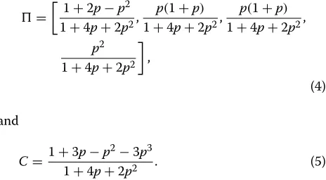
The sender may transmit a coded packet only when the system is at state S4. Indeed, at this state a clique is formed. At all other states there is no clique, and the greedy scheme would transmit a random uncoded packet. The system state transitions matrix and reward vector were given in Table 4 (“coded transmission”). With the transition matrix at hand, it is easy to devise the system stationary probabilities , as well as the average system rewardC(i.e., system capacity in packets per slot). For the symmetric case ofpa=pb=p,
=
1+2p−p2
1+4p+2p2,
p(1+p) 1+4p+2p2,
p(1+p) 1+4p+2p2, p2
1+4p+2p2
,
(4)
and
C= 1+3p−p 2−3p3
1+4p+2p2 . (5)
In the semi-greedy algorithm, the difference is in states
S2andS3. InS2(S3), an uncoded packet is sent to userb (a) with probability 1. The system state transitions matrix and reward vector are given in Table 7.
Table 7 State transitions for the two terminal case: semi-greedy scheme
State transition matrixPπˆ Reward vectorrπˆ
⎛ ⎜ ⎜ ⎜ ⎜ ⎜ ⎝ 1
2[(1−pa)+(1−pb)]+papb 12pa(1−pb) 21(1−pa)pb 0
0 (1−pb)+papb 0 (1−pa)pb
0 0 (1−pa)+papb pa(1−pb)
(1−pa)(1−pb) pa(1−pb) (1−pa)pb papb
⎞ ⎟ ⎟ ⎟ ⎟ ⎟ ⎠
⎛ ⎜ ⎜ ⎜ ⎜ ⎜ ⎝ 1
2(2−pa−pb) 1−pb
1−pa 2−pa−pb
The following equations depicts the stationary proba-bilities and the average capacity for the symmetric case of
pa=pb=p,
=
1−p
2+p,
1+p
4+2p), 1+p
4+2p), p
2+p
, (6)
and,
C= 2−2p
2
2+p . (7)
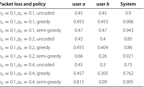
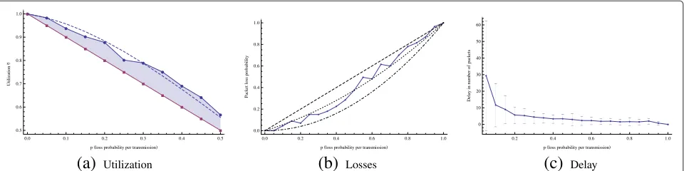
We can now compare the system capacity obtained with the greedy and the semi-greedy scheme relatively to the average capacity of an uncoded scheme. Figure 1a,b depict the system capacity gain as a function of the error prob-abilitiespaandpb. Table 8 depicts the users and system
capacity, for various error probability values, for the (i) uncoded case, (ii) the greedy scheme, and (iii) the semi-greedy scheme. The figures in the table clearly show the advantage of the semi-greedy scheme in terms of system capacity. Notice that the first rows in Table 8 are identical to the first rows of Table 6 up to a factor of1−1γ, which is exactly the sum of the geometric series of the discounted reward factorγ.
It is clear by now that the semi-greedy scheme obtains a higher capacity than the uncoded as well as the greedy schemes. Proposition 1 indicates that, for the two users case with a symmetric channel, i.e.,pa = pb = p, this
policy is optimal in terms of maximal average capacity (reward).
Proposition 1.Consider the two users case with a single packet buffer size. The Semi-Greedy Policy is the opti-mal among all policies in terms of maximizing the aver-age capacity.
Table 8 Two users capacity values
Packet loss and policy usera userb System
pa=0.1,pb=0.1, uncoded 0.45 0.45 0.9
pa=0.1,pb=0.1, greedy 0.453 0.453 0.906
pa=0.1,pb=0.1, semi-greedy 0.47 0.47 0.943
pa=0.1,pb=0.2, uncoded 0.45 0.4 0.85
pa=0.1,pb=0.2, greedy 0.455 0.404 0.86
pa=0.1,pb=0.2, semi-greedy 0.66 0.26 0.921
pa=0.1,pb=0.4, uncoded 0.45 0.3 0.75
pa=0.1,pb=0.4, greedy 0.457 0.305 0.762
pa=0.1,pb=0.4, semi-greedy 0.815 0.09 0.905
Proof.Intuitively, under our setting of a single packet buffer size, each packet should be transmitted uncoded at least once. Then, it could be retransmitted in coded pack-ets. To maximize the average capacity, an optimal policy would minimize the additional uncoded retransmissions. Clearly, the semi-greedy scheme obtains this by sending each packet uncoded only once and sending all retrans-missions coded. In addition, from a symmetry reasoning, at state S0 it does not matter whether to transmit to useraorb. Accordingly, the semi-greedy policy transmits either to useraorbat equal probabilities. More formally, the proposition follows from the dynamic programming optimality equation (i.e., Bellman’s equation) [5].
4.4 Fairness
Also clear from Table 8, is the potential unfairness of the semi-greedy scheme (unequal capacities due to unequal loss probabilities). As discussed previously, the semi-greedy scheme increases the system capacity by both
0.0
0.5
1.0 pa
0.0 0.5
1.0
pb
1.00 1.05 1.10 1.15
Gain
(a)
0.0
0.5
1.0 pa
0.0 0.5
1.0
pb
1.0 1.5 Gain
maximizing the usage of coded retransmission as well as byopportunistically transmitting to terminals with higher success probabilities. Indeed, users with worse channel conditions may suffer from a short time fairness. With mobile users, it is expected that their channel condition would vary such that the long term fairness prevails.
However, a more rigorous solution to the problem is possible, even for the case when mobility alone does not suffice. To see this, consider the expected, cumula-tivereward vector of the semi-greedy scheme in Table 7. For pa < pb, it is clear that maximizing the reward
results in preferring state S3 over S2, i.e., the system is biased towards useradecoding its packets. Nevertheless, an important benefit of the MPD-based approach in this article, is that this bias can be canceled using an appropri-ate weighting of the rewardgiven for each transition. By increasing the rewardgiven for decoding a packet by user b, compared to the reward given for decoding by usera, one can create an artificial bias towards userb. In fact, similar reward weighting can be used to imposequality of service
constraints or any other fairness mechanism.
4.5 Missing acknowledgements
The schemes suggested in this article utilize an Automatic Repeat reQuest (ARQ) mechanism which is compliant with IEEE 802.11. Nevertheless, it is important to note that the requirement that packets be acknowledged imme-diately (which is mandatory for the IEEE 802.11 protocol) is not compulsory in our scheme which can tolerate some delay between the packet and its corresponding ACK. Accordingly, if a certain delay is acceptable, the access point can act according to reports received from the users, once such reports are indeed received, and send the right coded packets. Of course, this requires larger buffers at the stations. Furthermore, it is also important to note that the assumption that acknowledgements sent by the receivers are received correctly by other receiving stations is not mandatory and was made only for the sake of sim-plicity. Specifically, receiving the acknowledgments by the users is required only in order for a user to know if a packet intended to a different user should be kept or dis-carded. Thus, if an acknowledgement sent by a user is not received by other users, the uninformed users keep obsolete packets. Such packets could be discarded after a certain timeout, or once these users identify newer pack-ets are being sent (by examining a sequence number in a packet). Hence, if users do not receive acknowledgements sent by others, there is no degradation in performance, only a requirement for slightly longer buffers.
The access point uses the acknowledgements in order to assess the state. Misinterpretation of the state can result in degradation of performance. Nevertheless, the theory of MDP includes well-established algorithms for cases when the state is only partially observed [38,39]. If the
observation of the state is kept within some mild fidelity from the true state, these algorithms perform very well. Furthermore, in a WiFi architecture, which is at the basis of this article, immediate acknowledgements are compul-sory, and the protocol does not function without a bidi-rectional communication between the access point and the user. Hence, assuming acknowledgements are received properly at the access point is reasonable.
5 Numerical analysis
In this section, we evaluate and compare theGreedyand
Semi-greedyalgorithms by simulation. We show that both algorithms significantly improve the performance com-pared to the uncoded version. Furthermore, we test the algorithms in various channel conditions, and examine fairness issues and their ability to adjust to varying condi-tions. This implementation also verifies that the proposed algorithms can be executed for a large number of users, compared to the prohibitive complexity of listing the entire state space.
We implemented the two algorithms in MATLAB. We modeled the channel between the AP and useriaccording to Bernoulli distribution with parameterpi. Accordingly,
user i receiveseach transmitted packet with probability 1 −pi. We further assumed small coherence time (fast
fading), i.e., the loss probability between two subsequent transmissions is i.i.d. and non-correlated channels, i.e., the loss probability between two different users is inde-pendent. Since both algorithms rely on finding the largest cliques in the graph induced by the state matrix, which as previously explained is known to be NP-complete in general, we have used the MATLAB function [40], which allows bounding the maximal clique size, hence bound the complexity according to Lemma 2. As baseline for comparison we used the traditional uncoded case.
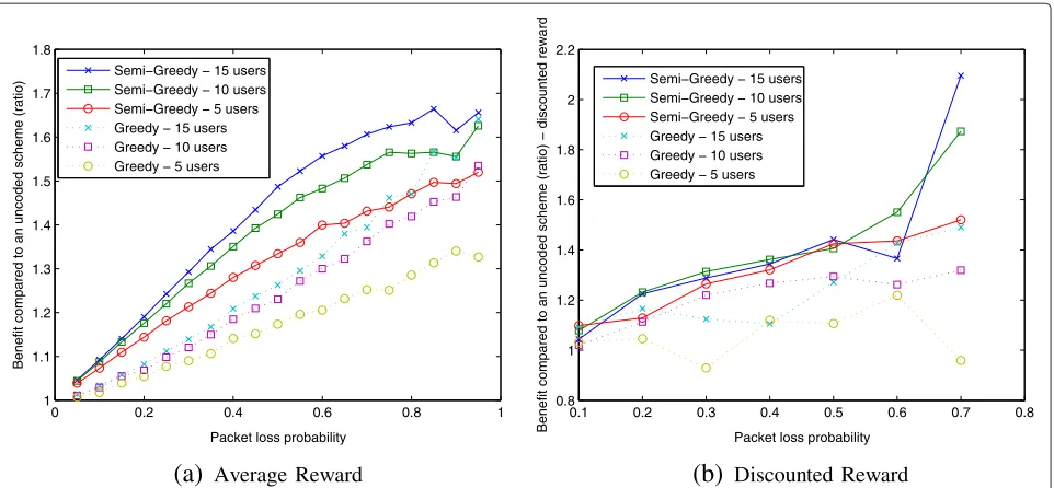
We start by investigating the gain of the two algorithms as a function of number of users and as a function of loss probability. Accordingly, we varied the number of users between 5, 10, and 15 and assumed that the AP always has traffic to send to each user. For each different number of users, we examined the performance for various loss prob-abilitiesp, ranging between 0.05 to 0.95 (for completeness we ran each set up for all loss probabilities, including very high ones, even though such loss probabilities are not common in real networks). Each setup was run for 20000 cycles. The results are depicted in Figure 2a.
0 0.2 0.4 0.6 0.8 1 1
1.1 1.2 1.3 1.4 1.5 1.6 1.7 1.8
Packet loss probability
Benefit compared to an uncoded scheme (ratio)
Semi−Greedy − 15 users Semi−Greedy − 10 users Semi−Greedy − 5 users Greedy − 15 users Greedy − 10 users Greedy − 5 users
(a)
Average Reward0.1 0.2 0.3 0.4 0.5 0.6 0.7 0.8
0.8 1 1.2 1.4 1.6 1.8 2 2.2
Packet loss probability
Benefit compared to an uncoded scheme (ratio) − discounted reward
Semi−Greedy − 15 users Semi−Greedy − 10 users Semi−Greedy − 5 users Greedy − 15 users Greedy − 10 users Greedy − 5 users
(b)
Discounted RewardFigure 2The benefit in the Semi-Greedy and Greedy approaches compared to the uncoded scheme.(a)Average reward (γ=1, normalized by the number of cycles).(b)Discounted reward (γ=0.95).
loss probability the higher the coding opportunities, hence the higher the gains. For example for 10 users and loss probability of 0.5 the gain over the uncoded scheme is 23% and 42%, for thegreedyandsemi-greedyalgorithms, respectively. Since the same holds also for number of users, i.e., the higher the number of users the greater the coding opportunities, the gain is an increasing function of the number of users. Furthermore, even though both algorithms offer high gains over the uncoded scheme,
Figure 2a clearly depicts that the semi-greedyalgorithm provides much higher gains than those of thegreedy algo-rithm. For example, for loss probability of 0.3 the gain of thesemi-greedyalgorithm is 2.2 times, 2.4 times and 2.1 times higher than those of thegreedyalgorithm, for the 5, 10, and 15 users, respectively.
To better understand the gain of the two algorithms, Figure 3 shows the average rewards seen by each user, for the 15 users setup for different loss probabilities (the
1 2
0 0.2 0.4 0.6 0.8 1 1.2 1.4
(a)
Packet loss probability 0.251 2
0 0.1 0.2 0.3 0.4 0.5 0.6 0.7 0.8 0.9 1
left bars correspond to the greedy algorithm and the right to the semi-greed). Each bar in the histogram represents the average reward seen by each user, where the average reward obtained by each user is normalized with respect to the number of users. The vertical line represents the average reward per transmission for the uncoded case. As can be seen in the figure, the average reward seen by each user is high compared to the uncoded case for all loss probabilities for both algorithms. Recall that the expected reward for packets which are sent uncoded for both algo-rithms is(1−p), which equals the one seen by the uncoded approach. It is interesting to note that variance of average reward obtained by different users is quite high.
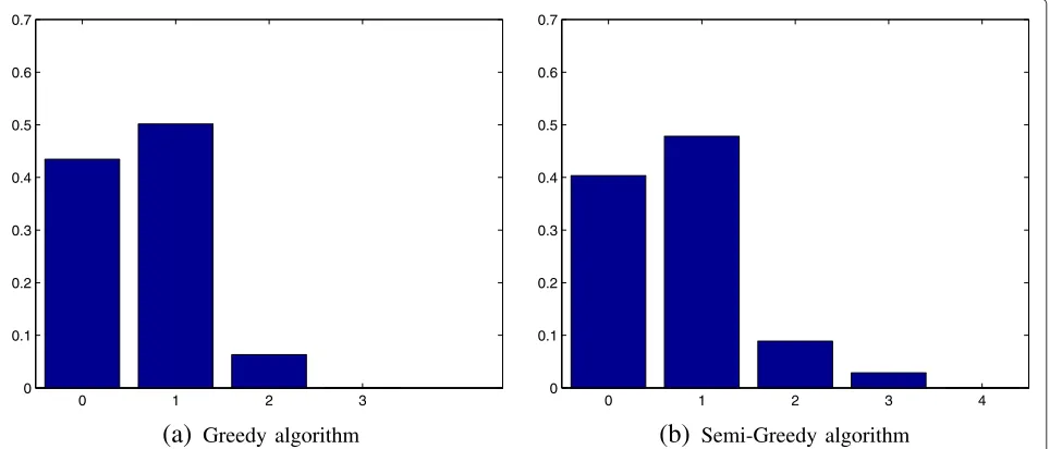
Next, we examined the rewards per transmission. Figure 4 shows a reward distribution comparison between the two algorithms for loss probability of 0.5 and 15 users. As expected, the semi-greedy algorithm yields greater average reward per transmission, confirming its superior-ity in terms of throughput gain over thegreedyalgorithm. Note also that the reward is a lower bound on the clique size to which the coded packet was transmitted. That is, the reward distribution gives good indication regarding the number of packets XORed in a coded packet, and a good indication regarding the sparseness of the matrix, and accordingly the complexity of finding the cliques. As can be seen in the figure, for both algorithms the matrices are relatively sparse.
Figure 2b depicts the asymptotic cumulativediscounted
reward of the system whenγ = 0.95 for thesemi-greedy
and the greedy approaches compared to the uncoded scheme. The dependency on the error probability, the benefit over the uncoded scheme and the benefit of the
semi-greedy algorithm over the greedy one are similar to those seen in the average reward setting. Note, however, that due to the exponential discount, results are effectively averaged over a much smaller window size, and hence are noisier.
Next, we compared the two algorithms when the chan-nels experienced by different users were not identical, i.e., different loss probabilities for different users. We ran a setup of ten users, where each user had different loss probability. Specifically, the loss probability ranged from 0.05 for user 1 to 0.5 for user 10. Figure 5 depicts the results where thex-axis presents the user I.D. (which cor-responds to the loss probability, i.e., loss probability = 0.05 ·userID). The y-axis depicts the normalized user throughput.
As can be seen, regarding throughput, thesemi-greedy
algorithm provides a higher average throughput, nonethe-less, regarding fairness, the greedy algorithm is much more fair than thesemi-greedyone. Thegreedyalgorithm distributes the throughput quite evenly, giving only slight advantage to users with low loss probability, e.g., the users with 0.05 and 0.5 loss probabilities get throughput of 0.08 and 0.06, respectively. The semi-greedy algorithm gives many more transmission opportunities to users with good channel quality (low loss probability).
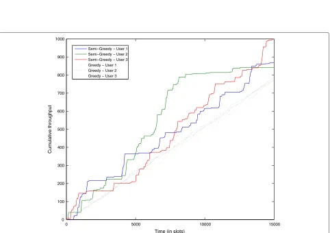
Finally, we continued examining the performance of the two algorithms when the user’s loss probabilities were not constant. We modeled each channel as a Markov chan-nel, where the channel of each user alternated between good and bad. The loss probabilities were 0.05 and 0.5 for the good and bad channels, respectively. The transi-tion probability between the two states was 0.01. Figure 6
0 1 2 3
0 0.1 0.2 0.3 0.4 0.5 0.6 0.7
(a)
Greedy algorithm0 1 2 3 4
0 0.1 0.2 0.3 0.4 0.5 0.6 0.7
(b)
Semi-Greedy algorithm1 2 3 4 5 6 7 8 9 10 0
0.05 0.1 0.15 0.2 0.25 0.3 0.35 0.4 0.45 0.5
(a)
Greedy algorithm1 2 3 4 5 6 7 8 9 10
0 0.05 0.1 0.15 0.2 0.25 0.3 0.35 0.4 0.45 0.5
(b)
Semi-Greedy algorithm Figure 5User throughput with unequal packet loss probabilities.Probabilities range from 0.05 for user 1 to 0.5 for user 10.(a)Greedy algorithm.(b)Semi-Greedy algorithm.0 5000 10000 15000
0 100 200 300 400 500 600 700 800 900 1000
Time (in slots)
Cumulative throughput
Semi−Greedy − User 1 Semi−Greedy − User 2 Semi−Greedy − User 3 Greedy − User 1 Greedy − User 2 Greedy − User 3