Optimizing Resource Management in Cloud Analytics Services

(1)

Services

Thesis by

Xiaoqi Ren

In Partial Fulfillment of the Requirements for the Degree of

Doctor of Philosophy

CALIFORNIA INSTITUTE OF TECHNOLOGY Pasadena, California

2018

(2)

ORCID: 0000-0002-1121-9046

(3)

ACKNOWLEDGEMENTS

First, I would like to express my deepest gratitude to my advisor, Professor Adam Wierman. He has been a great advisor to me throughout my Ph.D. It is really an invaluable experience working with him and learning from him. He has always been enthusiastic about research. He encouraged us to explore projects based on our interests instead of being driven by funding. He engaged deeply into our projects and provided excellent guidance. His insightful vision, rigorous thinking, and effective presentations have profoundly influenced me to be a better scholar. Professor Wierman always supported me to overcome the obstacles and encouraged me to be brave and step out of my safe zone. He also gave enormous help with planning my career path. I sincerely appreciate the amazing impact he has had on me, which makes me stronger and more confident as a researcher.

Next, I would like to thank my thesis committee members, Professor Steven Low, Professor Mani Chandy and Professor Yisong Yue, for all of their guidance through this process. Their ideas and feedbacks have been absolutely invaluable. Also, I am grateful to my mentors during my internships at Microsoft Research: Yuxiong He, Sameh Elnikety, Kathryn S McKinley and Christian Konig. And I would like to thank my collaborators: Palma London, Juba Ziani, Mohammad A. Islam, Shaolei Ren, Xiaorui Wang, Ganesh Ananthanarayanan, Minlan Yu, Niangjun Chen, Michael Chien-Chun Hung, and Ion Stoica. It has been a great pleasure to work with them. They have always provided insightful discussions and constructive suggestions.

I have greatly enjoyed the opportunity to study in the Department of Computing and Mathematical Sciences at Caltech, which provides a supportive environment in which students can fully focus on research. It is wonderful to interact with so many intelligent professors and outstanding students. I would also like to thank the helpful administrative staff in our department, especially Sheila Shull, Sydney Garstang, and Maria Lopez.

(4)

ABSTRACT

The fundamental challenge in the cloud today is how to build and optimize machine learning and data analytical services. Machine learning and data analytical platforms are changing computing infrastructure from expensive private data centers to easily accessible online services. These services pack user requests as jobs and run them on thousands of machines in parallel in geo-distributed clusters. The scale and the complexity of emerging jobs lead to increasing challenges for the clusters at all levels, from power infrastructure to system architecture and corresponding software framework design.

These challenges come in many forms. Today’s clusters are built on commodity hardware and hardware failures are unavoidable. Resource competition, network congestion, and mixed generations of hardware make the hardware environment complex and hard to model and predict. Such heterogeneity becomes a crucial roadblock for efficient parallelization on both the task level and job level. Another challenge comes from the increasing complexity of the applications. For example, machine learning services run jobs made up of multiple tasks with complex de-pendency structures. This complexity leads to difficulties in framework designs. The scale, especially when services span geo-distributed clusters, leads to another important hurdle for cluster design. Challenges also come from the power infras-tructure. Power infrastructure is very expensive and accounts for more than 20% of the total costs to build a cluster. Power sharing optimization to maximize the facility utilization and smooth peak hour usages is another roadblock for cluster design. In this thesis, we focus on solutions for these challenges at the task level, on the job level, with respect to the geo-distributed data cloud design and for power management in colocation data centers.

(5)

EC2 cluster of 200 nodes show that GRASS increases accuracy of deadline-bound jobs by 47% and speeds up error-bound jobs by 38%.

Moving from task level to job level, task level speculation mechanisms are designed and operated independently of job scheduling when, in fact, scheduling a specu-lative copy of a task has a direct impact on the resources available for other jobs. Thus, we present Hopper, a job-level speculation-aware scheduler that integrates the tradeoffs associated with speculation into job scheduling decisions based on a model generalized from the task-level speculation model. We implement both cen-tralized and decencen-tralized prototypes of the Hopper scheduler and show that 50% (66%) improvements over state-of-the-art centralized (decentralized) schedulers and speculation strategies can be achieved through the coordination of scheduling and speculation.

As computing resources move from local clusters to geo-distributed cloud services, we are expecting the same transformation for data storage. We study two crucial pieces of a geo-distributed data cloud system: data acquisition and data placement. Starting from developing the optimal algorithm for the case of a data cloud made up of a single data center, we propose a near-optimal, polynomial-time algorithm for a geo-distributed data cloud in general. We show, via a case study, that the resulting design, Datum, is near-optimal (within 1.6%) in practical settings.

(6)

PUBLISHED CONTENT AND CONTRIBUTIONS

[1] G. Ananthanarayanan, M. C. Hung, X. Ren, I. Stoica, A. Wierman, and M. Yu. “GRASS: Trimming Stragglers in Approximation Analytics”. In:

Proceedings of the 11th USENIX Conference on Networked Systems Design and Implementation. NSDI’14. Seattle, WA: USENIX Association, 2014, pp. 289–302. isbn: 978-1-931971-09-6.

Adapted into Chapter 2 of this thesis. X. Ren contributed to the conception of the project, proposing the model and analyzing the performance, and writing the manuscript.

[2] X. Ren, G. Ananthanarayanan, A. Wierman, and M. Yu. “Hopper: Decen-tralized Speculation-aware Cluster Scheduling at Scale”. In:Proceedings of the 2015 ACM Conference on Special Interest Group on Data Communica-tion. SIGCOMM ’15. London, United Kingdom: ACM, 2015, pp. 379–392. isbn: 978-1-4503-3542-3. doi: 10.1145/2785956.2787481.

[3] X. Ren, P. London, J. Ziani, and A. Wierman. “Datum: Managing Data Purchasing and Data Placement in a Geo-Distributed Data Market”. In:

IEEE/ACM Transactions on Networking 26.2 (2018), pp. 893–905. doi: 10.1109/TNET.2018.2811374.

[4] N. Chen, X. Ren, S. Ren, and A. Wierman. “Greening Multi-Tenant Data Center Demand Response”. In: SIGMETRICS Perform. Eval. Rev. 43.2 (Sept. 2015), pp. 36–38. issn: 0163-5999. doi: 10.1145/2825236.2825252. Adapted into Chapter 5 of this thesis. X. Ren contributed to the conception of the project, proposing the model and analyzing the performance, and writing the manuscript.

[5] M. A. Islam, X. Ren, S. Ren, A. Wierman, and X. Wang. “A market approach for handling power emergencies in multi-tenant data center”. In: High Per-formance Computer Architecture (HPCA), 2016 IEEE International Sym-posium on. IEEE. 2016, pp. 432–443. doi: 10.1109/HPCA.2016.7446084. url: https://ieeexplore.ieee.org/document/7446084/.

(7)

LIST OF ILLUSTRATIONS

Number Page

2.1 GS and RAS for a deadline-bound job with 9 tasks. The tremand tnew values are when T2 finishes. The example illustrates deadline values of 3 and 6 time units. . . 15 2.2 GS and RAS for error-bound job with 6 tasks. The trem and tnew

values are when T2 finishes. The example illustrates error limit of 40% (3 tasks) and 20% (4 tasks). . . 18 2.3 Hill plot of Facebook task durations. . . 19 2.4 Near-optimality of GS & RAS under Pareto task durations (β= 1.259). 23 2.5 Accuracy Improvement in deadline-bound jobs with LATE [18] and

Mantri [17] as baselines. . . 30 2.6 GRASS’s overall gains (compared to LATE) binned by the deadline

and error bound. Deadlines are binned by the factor over ideal job duration (see Section 2.6.1) . . . 31 2.7 Speedup in error-bound jobs with LATE [18] and Mantri [17] as

baselines. . . 32 2.8 GRASS’s gains matches the optimal scheduler. . . 33 2.9 GRASS’s gains hold across job DAG sizes. . . 33 2.10 GRASS’s switching is 25% better than using GS or RAS all through

for deadline-bound jobs. We use the Facebook workload and LATE as baseline. . . 34 2.11 GRASS’s switching is 20% better than using GS or RAS all through

for error-bound jobs. We use the Facebook workload and LATE as baseline. . . 34 2.12 Comparing GRASS’s learning based switching approach to a

straw-man that approximates two waves of tasks. GRASSis 30%−40% better than the strawman. . . 35 2.13 Using all three factors for deadline-bound jobs compared to only one

or two is 18%−30% better. . . 36 2.14 Using all three factors for error-bound jobs compared to one or two

(10)

2.15 Sensitivity of GRASS’s performance to the perturbation factor ξ. Usingξ =15% is empirically best. . . 37 3.1 Combining SRPT scheduling and speculation for two jobs A (4 tasks)

and B (5 tasks) on a 7-slot cluster. The + suffix indicates speculation. Copies of tasks that are killed are colored red. . . 43 3.2 Hopper: Completion time for jobs A and B are 12 and 22. The +

suffix indicates speculation. . . 44 3.3 The impact of number of slots on single job performance. The

number of slots is normalized by job size (number of tasks within the job). β is the Pareto shape parameter for the task size distribution. (In our traces 1 < β < 2.) The red vertical line shows the threshold point. . . 49 3.4 Decentralized scheduling architecture. . . 68 3.5 The impact of number of probes and number of refusals onHopper’s

performance. . . 69 3.6 Hopper’s gains with cluster utilization. . . 76 3.7 Hopper’s gains by job bins over Sparrow-SRPT. . . 77 3.8 (a) CDF of Hopper’s gains, and (b) gains as the length of the job’s

DAG varies; both at 60% utilization. . . 78 3.9 Hopper’s results are independent of the straggler mitigation strategy. . 79 3.10 Fairness. Figure (a) shows sensitivity of gains to. Figure (b) shows

the fraction of jobs that slowed down compared to a fair allocation, and (c) shows the magnitude of their slowdowns (average and worst). 80 3.11 Power ofdchoices: Impact of the number of probes on job completion. 80 3.12 Centralized Hopper’s gains over SRPT, overall and broken by DAG

length (Facebook workloads). . . 81 3.13 Centralized Hopper: Impact of Locality Allowance (k) (see

(11)

4.1 An overview of the interaction between data providers, the data cloud, and clients. The dotted line encircling the data centers (DC) repre-sents the geo-distributed data cloud. Data providers and clients inter-act only with the cloud. Data providerpsends data of qualityq(l,p)

to data centerd, and the corresponding operation cost isβp,d(l)yp,d(l).

Similarly, data center d sends data of quality q(l,p) to client c, and the corresponding execution cost is αd,c(l,p)xd,c(l,p). In bulk

data contracting, the corresponding purchasing cost is f(l,p)z(l,p). In per-query data contracting, the corresponding purchasing cost is

f(l,p)xd,c(l,p). . . 95

4.2 Illustration of the near-optimality ofDatumas a function of the com-plexity of client requests (i.e., the average number of providers data must be procured from in order to complete a client request). . . 112

4.3 Illustration ofDatum’s sensitivity to query parameters. (a) varies the heaviness of the tail in the distribution of purchasing fees. (b) varies the number of quality levels available. Note that Figure 4.2 sets the shape parameter of the Pareto governing purchasing fees to 2 and includes 8 quality levels. . . 114

4.4 Illustration of the impact of bandwidth and purchasing fees onDatum’s performance. NearestDC is excluded because its costs are off-scale. (a) varies the ratio of bandwidth costs (summarized by α+ β) to purchasing costs (summarized by f). (b) varies the ratio of costs internal to the data cloud (α) to costs external to the data cloud (β+ f). Note that in Figure 4.2 the ratios are set to log(α+_fβ)= −0.5 and log(_β₊α_f)=−1. . . 115

5.1 Data center infrastructure. . . 123

5.2 CDF of measured power usage. . . 124

5.3 Illustration of tenant’s bidding. . . 153

5.4 API diagram forCOOP. . . 156

5.5 Power and performance models. . . 161

5.6 Cost models. . . 161

5.7 Comparison of different algorithms. . . 165

5.8 Power traces under different oversubscription configurations. . . 165

5.9 Delay performance traces of the tenants under different oversubscrip-tion levels. . . 165

(12)

(13)

LIST OF TABLES

Number Page

2.1 Details of Facebook and Bing traces. . . 29 3.1 Task sets. torig andtnew are durations of the original and speculative

copies of each task. . . 44 5.1 Analysis of Capacity Oversubscription. . . 126 5.2 Performance guarantee of COOP compared to the social optimal

(14)

Chapter 1

INTRODUCTION

In the last two decades, the emerging of big data has driven enormous push in the technology developments of both distributed systems and machine learning. In the era of big data, the requirement to provide predictable and scalable services has led to a remarkable evolution of large scale data analytics frameworks. From MapReduce [1] to Spark [2] then to Flink [3], from support for simple batch jobs to support for steam processing to integrated machine learning and graph libraries, there is a trend towards broader and more general system design. Meanwhile, the fast evolution of system frameworks inevitably leads to significant challenges from scalability to compatibility with existing systems and new applications. In the following, we first investigate the evolution of the data analytics frameworks , and then highlight the challenges to the design of large scale data analytics frameworks. Finally we give an overview of the contributions this thesis make toward these challenges.

1.1

The Evolution of Large Scale Data Analytics Frameworks

(15)

MapReduce quickly expanded beyond Google. In 2006, Hadoop [4], an open source version of MapReduce, was developed by Doug Cutting and Mike Cafarella. The core of Hadoop consists of two parts, (1) the storage architecture, Hadoop Distributed File System (HDFS) [5], which is inspired by the Google File System (GFS) [6], and (2) the processing model, MapReduce. Hadoop MapReduce quickly became the most popular open source implementation of MapReduce. Yahoo!, Facebook and many others soon adopted Hadoop to build their large cloud computing clusters [7]. In 2010, Facebook announced that they had the largest Hadoop cluster in the world with 21 PB of storage. The data volume had grown to 100 PB in mid 2012 and was reported to continuously grow by roughly half a PB per day later that year. Hadoop adoption had become widespread as of 2013: more than half of the Fortune 50 used Hadoop [8].

As Hadoop became widely used, the early adopters started to notice the limita-tions of the classical MapReduce framework, including lack of scalability, resource underutilization and the lack of support for complex applications.

These issues are mainly due to two design choices. (1) MapReduce uses a single centralized JobTracker process to constantly track all the resource management and allocation and perform coordination of all jobs and their tasks running on the cluster. Besides the JobTracker, a number of TaskTracker processes are used to assign tasks and periodically report the progresses to the JobTracker. The highly centralized structure of the JobTracker results in scalability issue, especially for real time data analytics. (2) To ease the workload of the JobTracker and TaskTracker, in MapReduce the computational resources on each node are divided into fixed number of map slots and reduce slots, which lead to significant resource underutilization, especially when a job requires an unequal number of mappers and reducers.

(16)

other Hadoop modules) become the core modules of the Apache Hadoop project [4]. While MapReduce is well suited for batch processing, its deficiency for real time data analytics on complicated applications, especially for applications that reuse the same working set of data across multiple MapReduce jobs, is also widely noticed by researchers and developers. For example, iterative machine learning jobs experience significant delay in MapReduce because each iteration is considered as an individual MapReduce job and, in the MapReduce framework, each job must load data from the disk independently. To handle this challenge, M. Zaharia et al. developed Apache Spark in 2010 [2]. Spark shares a similar programming model to MapReduce, but adopts an abstraction called resilient distributed dataset (RDD) which allows users to explicitly cache data sets in memory across machines and reuse them across multiple MapReduce jobs (MapReduce-like parallel operations). Spark can run either in stand-alone mode or combined with Hadoop as a replacement for MapReduce. Unlike MapReduce which is best suited for batch processing, Spark is designed to handle both batch processing and stream processing. Its in-memory data processing ensures fast speed and thus makes Spark one of the most popular real time data analytic frameworks.

(17)

1.2

Challenges to the Design of Analytics Frameworks

Even with the success of existing various industrial systems, as the volume of data continues to grow, the scale of the clusters expands and complicated applications impose new requirements on the systems, which lead to new challenges to the design of analytics frameworks.

One significant goal for data analytics frameworks is to provide predictable perfor-mance. As the scale and complexity of clusters increase, hard-to-model systemic interactions that degrade the performance of tasks become common. Consequently, many tasks become “stragglers”, i.e., running slower than expected, leading to significant unpredictability (and delay) in job completion times. Dealing with strag-glers is a crucial design component that has received widespread attention across prior studies [15, 16]. The dominant technique to mitigate stragglers is specula-tion, which works by launching speculative copies for the slower tasks, where a speculative copy is simply a duplicate of the original task. It then becomes a race between the original and the speculative copies. Such techniques are state of the art and deployed in production clusters at Facebook and Microsoft Bing, thereby significantly speeding up jobs [1, 15, 17, 18]. However, current straggler mitigation algorithms are mainly focused on the task level without considering how specula-tion will affect job level scheduling. Speculaspecula-tion policies deployed today are all designed and operated independently of job scheduling; schedulers simply allocate slots to speculative copies in a best-effort" fashion, e.g., [1, 17, 19, 20]. Also the existing speculation algorithms are lack of support for complicated job structures, such as DAG, and only focus on performing speculation mitigation on current wave of tasks [1, 17, 19].

(18)

Such approximation jobs require schedulers to prioritize the appropriate subset of their tasks depending on the approximation criteria, while distributed systems are generally designed to evenly prioritize each tasks. Balancing between these two provides new challenges for system design.

Achieving lower latency is an increasing challenge as large scale data analytics frameworks are shifting towards shorter task duration and higher degrees of paral-lelization. In 2004, the scale of task duration was more than 10 min, while in 2010, for Spark in memory query, the scale of task duration was already shortened to hun-dreds of milliseconds [20]. We expect the trend to continue in the future generations of frameworks with task duration being even smaller. In this situation, controlling system overheads becomes of importance for real time data analytics design. To-day’s state-of-the-art frameworks use distributed schedulers to achieve lightweight scheduling while maintaining low latency [16, 20, 24]. In such frameworks, each scheduler only knows partial information about jobs and working machines. Opti-mizing such systems, especially with regards to efficient straggler mitigation, is still challenging.

The most widely used scheduling approach in clusters today is based on fairness, which can be thought of as equal sharing (or weighted sharing) of the available resources among jobs (or cluster users) [25]. The equal sharing strategy guarantees isolation in resource management, in the sense that users are guaranteed to receive their fair shares and no starvation can exist. However, fairness, of course, comes with the cost of performance inefficiencies. How to balance fairness and efficiency to avoid starvation for jobs while achieving high efficiency is another system design challenge.

(19)

consumption for a short period of time with power techniques such as load migra-tion/scheduling [38]. Such flexibility makes data centers promising resources for demand response, particularly for emergency demand response, which saves the power grid from incurring blackouts during emergency situations. Existing studies mostly focus on owner operated data centers (e.g., Google) whose operators have full control over both servers and facilities. But multi-tenant colocation data centers have been investigated much less frequently. In a colocation data center (simply called “colocation” or “colo”), multiple tenants deploy and keep full control of their own physical servers in a shared space, while the colo operator only provides facility support (e.g., high-availability power and cooling). Colos are less studied than owner-operated data centers, but they are actually more common in practice. Colos offer data center solutions to many industry sectors, and serve as physical home to many private clouds, medium-scale public clouds (e.g., VMware) [39], and content delivery providers (e.g., Akamai). Further, a recent study shows that colos consume nearly 40% of data center energy in the U.S., while Google-type data centers collectively account for less than 8%, with the remaining going to enterprise in-house data centers [40]. With such huge potential, efficient power management for colos becomes an important challenge in data center design.

1.3

Overview of This Thesis

This thesis is divided into four components. In Chapter 2, we focus on the task-level data analytics framework optimization for approximation jobs. In Chapter 3, we study the job-level optimization with a joint design of job scheduling and speculation mitigation. In Chapter 4, we investigate the design of the geo-distributed data cloud with joint optimization of data acquisition and data placement. Finally in Chapter 5, we study power management in collocation data centers.

Chapter 2: speculation-aware cluster scheduling at the task level

(20)

In this chapter, we presentGRASS, which carefully uses speculation to mitigate the impact of stragglers in approximation jobs. We develop an analytic model to analyze the optimal speculation level for approximation jobs. GRASS’s design is based on the guidelines derived from the analysis. GRASSdelicately balances immediacy of improving the approximation goal with the long term implications of using extra resources for speculation. Evaluations with production workloads from Facebook and Microsoft Bing in an EC2 cluster of 200 nodes shows that GRASSincreases accuracy of deadline-bound jobs by 47% and speeds up error-bound jobs by 38%. GRASS’s design also speeds up exact computations (zero error-bound), making it a

unified solution for straggler mitigation. This work summarizes the result in [19].

Chapter 3: speculation-aware cluster scheduling on the job level

In this chapter, we study the job-level data analytics framework optimization with a joint design of job scheduling and speculation mitigation. As clusters continue to grow in size and complexity, providing scalable and predictable performance is an increasingly important challenge. At this point, speculative execution has been widely adopted to mitigate the impact of stragglers. However, speculation mechanisms are designed and operated independently of job scheduling when, in fact, scheduling a speculative copy of a task has a direct impact on the resources available for other jobs. In this work, we present Hopper, a job scheduler that is speculation-aware, i.e., that integrates the tradeoffs associated with speculation into job scheduling decisions. We generalize the model in Chapter 2 from task level to job level and designHopperbased on that. A knob to balance fairness and efficiency and solutions to jobs with DAGs and heterogeneous jobs are also provided in the design. We implement both centralized and decentralized prototypes of theHopper scheduler and show that 50% (66%) improvements over state-of-the-art centralized (decentralized) schedulers and speculation strategies can be achieved through the

coordinationof scheduling and speculation. This work summarizes the result in [41].

Chapter 4: network-aware geo-distributed cluster scheduling

(21)

data cloud made up of a single data center, and then generalize the structure from the single data center setting in order to develop a near-optimal, polynomial-time algorithm for a geo-distributed data cloud. The resulting design,Datum, decomposes the joint purchasing and placement problem into two subproblems, one for data purchasing and one for data placement, using a transformation of the underlying bandwidth costs. We show, via a case study, that Datum is near-optimal (within 1.6%) in practical settings. This work summarizes the result in [42].

Chapter 5: Power Capping in Colocation Data Centers

(22)

Chapter 2

SPECULATION-AWARE CLUSTER SCHEDULING

AT THE TASK LEVEL

Large scale data analytics frameworks automatically compose jobs operating on large data sets into many smalltasksand execute them in parallel oncompute slots

on different machines. A key feature catalyzing the widespread adoption of these frameworks is their ability to guard against failures of tasks, both when tasks fail outright as well as when they run slower than the other tasks of the job. Dealing with the latter, referred to asstragglers, is a crucial design component that has received widespread attention across prior studies [15, 17, 18].

The dominant technique to mitigate stragglers isspeculation—launching speculative copies for the slower tasks, where a speculative copy is simply a duplicate of the original task. It then becomes a race between the original and the speculative copies. Such techniques are state of the art and deployed in production clusters at Facebook and Microsoft Bing, thereby significantly speeding up jobs.

Approximation jobs are starting to see considerable interest in data analytics clusters [21–23]. These jobs are based on the premise that providing a timely result, even if only on part of the dataset, is more important than processing the entire data. These jobs tend to have approximation boundson two dimensions—deadline and error [45]. Deadline-bound jobs strive to maximize the accuracy of their results within a specified time deadline. Error-bound jobs, on the other hand, strive to minimize the time taken to reach a specified error limit in the result. Typically, approximation jobs are launched on a large dataset and require only asubsetof their tasks to finish based on the bound [46–48].

Our focus in this chapter is on the problem of task-level speculation for

approx-imation jobs.1 Traditional speculation techniques for straggler mitigation face a 1_{Note that an error-bound job with error of zero is the same as an exact job that requires all}

(23)

fundamental limitation when dealing with approximation jobs, since they do not take into account approximation bounds. Ideally, when the job has many more tasks than compute slots, we want to prioritize those tasks that are likely to complete within the deadline or those that contribute the earliest to meeting the error bound. By not considering the approximation bounds, state-of-the-art straggler mitigation techniques in production clusters at Facebook and Bing fall significantly short of optimal mitigation. They are 48% lower in average accuracy for deadline-bound jobs and 40% higher in average duration of error-bound jobs.

Optimally prioritizing tasks of a job to slots is a classic scheduling problem with known heuristics [49–51]. These heuristics, unfortunately, do not directly carry over to our scenario for the following reasons. First, they calculate the optimal ordering statically. Straggling of tasks, on the other hand, is unpredictable and necessitates dynamic modification of the priority ordering of tasks according to the approximation bounds. Second, and most importantly, traditional prioritization techniques assign tasks to slots assuming every task occupies only one slot. Spawn-ing a speculative copy, however, leads to the same task usSpawn-ing two (or multiple) slots simultaneously. Hence, this distills our challenge to achieving the approximation bounds by dynamically weighing the gains due to speculation against the cost of

using extra resources for speculation.

Scheduling a speculative copy helps make immediate progress by finishing a task faster. However, while not scheduling a speculative copy results in the task running slower, many more tasks may be completed using the saved slot. To understand this

opportunity cost, consider a cluster with one unoccupied slot and a straggler task. Letting the straggler complete takes five more time units while a new copy of it would take four time units. While scheduling a speculative copy for this straggler speeds it up by one time unit, if we were not to, that slot could finish another task (taking five time units too).

This simple intuition of opportunity cost forms the basis for our two design proposals. First, Greedy Speculative (GS) scheduling is an algorithm that greedily picks the task to schedule next (original or speculative) that most improves the approximation goal at that point. Second, Resource Aware Speculative (RAS) scheduling considers the opportunity cost and schedules a speculative copy only if doing so saves both timeandresources.

(24)

our model is that the value of being greedy (GS) increases for smaller jobs while considering opportunity cost of speculation (RAS) helps for larger jobs. As our model is generic, a nice aspect is that the guideline holds not only for approximation jobs but also for exact jobs that require all their tasks to complete.

We use the above guideline to dynamically combine GS and RAS, which we call GRASS. At the beginning of a job’s execution,GRASSuses RAS for scheduling tasks. Then, as the job getscloseto its approximation bound, it switches to GS, since our theoretical model suggests that the opportunity cost of speculation diminishes with fewer unscheduled tasks in the job. GRASSlearns the point to switch from RAS to GS using job and cluster characteristics.

We demonstrate the generality of GRASS by implementing it in both Hadoop [4] (for batch jobs) and Spark [52] (for interactive jobs). We evaluate GRASS using production workloads from Facebook and Bing on an EC2 cluster with 200 machines. GRASS increases accuracy of deadline-bound jobs by 47% and speeds up error-bound jobs by 38% compared to state-of-the-art straggler mitigation techniques deployed in these clusters (LATE [18] and Mantri [17]). In fact, GRASS results in near-optimal performance. In addition, GRASS also speeds up exact jobs, that require all their tasks to complete, by 34%. Thus, it is aunified speculation solution for both approximation as well as exact computations.

2.1

Challenges and Opportunities

Before presenting our system design, it is important to understand the challenges and opportunities for speculating straggler tasks in the context of approximation jobs.

2.1.1 Approximation Jobs

Increasingly, with the deluge of data, analytics applications no longer require pro-cessing the entire datasets. Instead, they choose to trade off accuracy for response time. Approximate results obtained early from just part of the dataset are often

good enough[21–23]. Approximation is explored across two dimensions—time for obtaining the result (deadline) and error in the result [45].

(25)

systems and web search engines. Generally, the job is spawned on a large dataset and accuracy is proportional to the fraction of data processed [46–48] (or tasks completed, for ease of exposition).

• Error-boundjobs strive to minimize the time taken to reach a specified error limit in the result. Again, accuracy is measured in the amount of data processed (or tasks completed). Error-bound jobs are used in scenarios where the value in reducing the error below a limit is marginal,e.g.,counting the number of cars crossing a section of a road to the nearest thousand is sufficient for many purposes.

Approximation jobs require schedulers toprioritize the appropriate subset of their tasks depending on the deadline or error bound. Prioritization is important for two reasons. First, due to cluster heterogeneities [15, 18, 53], tasks take different durations even if assigned the same amount of work. Second, jobs are often multi-waved, i.e., their number of tasks is much greater than the available compute slots, thereby they run only a fraction of their tasks at a time [54]. For example, when a job with 1000 tasks is given only 100 slots simultaneously (due to, say, fair scheduling), it runs only one-tenth of its tasks at a time. These tasks, though, are independent and can be scheduled in any order. The trend of multi-waved jobs is expected to grow with smaller tasks [55].

2.1.2 Challenges

The main challenge in prioritizing tasks of approximation jobs arises due to some of themstraggling. Even after applying many proactive techniques, in production clusters in Facebook and Microsoft Bing, the average job’s slowest task is eight times slower than the median.2 It is difficult to model all the complex interactions in clusters to prevent stragglers [15, 57]. Ananthanarayanan et al. (Section 2.1.2 in [15]) also show that blacklisting machines based on their likeliness to cause stragglers (in both the short- as well as long-term) has little benefits; machines are neither consistently problematic nor exhibit simple correlations with task durations. The widely adopted technique to deal with straggler tasks isspeculation. This is a reactive technique that spawns speculative copies for tasks deemed to be straggling. The earliest among the original and speculative copies is picked while the rest are

(26)

killed. While scheduling a speculative copy makes the task finish faster and thereby increases accuracy, they also compete for compute slots with the unscheduled tasks. Therefore, our problem is todynamically prioritize tasks based on the deadline/error-bound while choosing between speculative copies for stragglers and unscheduled

tasks. This problem is, unfortunately, NP-Hard and devising good heuristics (i.e., with good approximation factors) is an open theoretical problem.

2.1.3 Potential Gains

Given the challenges posed by stragglers discussed above, it is not surprising that the potential gains from mitigating their impact are significant. To highlight this we use a simulator with an optimal bin-packing scheduler. Our baselines are the the state-of-the-art mitigation strategies (LATE [18] and Mantri [17]) in the pro-duction clusters. Optimally prioritizing the tasks while correctly balancing between speculative copies and unscheduled tasks presents the following potential gains. Deadline-bound jobs improve their accuracy by 48% and 44%, in the Facebook and Bing traces, respectively. Error-bound jobs speed up by 32% and 40%. We next develop two online heuristics to achieve these gains.

2.2

Speculation Algorithm Design

The key choice made by a cluster scheduling algorithm is to pick the next task to schedule given a vacant slot. Traditionally, this choice is made among the set of tasks that are queued; however when speculation is allowed, the choice also includes speculative copies of tasks that are already running. This extra flexibility means that a design must determine a prioritization that carefully weighs the gains from speculation against the cost of extra resources while still meeting the approximation goals. Thus, we first focus on tradeoffs in the design of the speculation policy. Specifically, using both small examples and analytic modeling we motivate the use of two simple heuristics, Greedy Speculative (GS) scheduling and Resource Aware Speculative (RAS) scheduling that together make up the core ofGRASS.

2.2.1 Speculation Alternatives

(27)

2.2.1.1 Deadline-bound Jobs

If speculation was not allowed, there is a natural, well-understood policy for the case of deadline-bound jobs: Shortest Job First (SJF), which schedules the task with the smallest processing time. In many settings, SJF can be proven to minimize the number of incomplete tasks in the system, and thus maximize the number of tasks completed, at all points of time among the class of non-preemptive policies [49, 50]. Thus, without speculation, SJF finishes the most tasks before the deadline.

If one extends this idea to the case where speculation is allowed, then a natural approach is to allow the currently running tasks to also be placed in the queue, and to choose the task with the smallest size, i.e., tnew(requiring, of course, that the task finishes before the deadline). If the chosen task has a copy currently running, we check that the speculative copy being considered provides a benefit, i.e., tnew <trem. So, the next task to run is still chosen according to SJF, only now speculative copies are also considered. We term this policy Greedy Speculative (GS) scheduling, because it picks the next task to schedule greedily, i.e., the one that will finish the quickest, and thus improve the accuracy the earliestat present.

Figure 2.1 (left) presents an illustration of GS for a simple job with nine tasks and two concurrent slots. Tasks T1 and T2 are scheduled first, and when T2 finishes, the trem and tnewvalues are as indicated. At this point, GS schedules T3 next as it is the one with the lowest tnew, and so forth. Assuming the deadline was set to 6 time units, the obtained accuracy is 7₉ (or 7 completed tasks).

Picking the earliest task to schedule next is often optimal when a job has no un-scheduled tasks (i.e., either single-waved jobs or the last wave of a multi-waved job). However, when there are unscheduled tasks it is less clear. For example, in Figure 2.1 (right) if we schedule a speculative copy of T1 when T2 finished, instead of T3, 8 tasks finish by the deadline of 6 time units.

The previous example highlights that running a speculative copy has resource im-plications which are important to consider. If the speculative copy finishes early, both slots (of the speculative copy and the original) become available sooner to start the other tasks. This opportunity cost of speculation is an important tradeoff to consider, and leads to the second policy we consider: Resource Aware Speculative (RAS) scheduling.

(28)

Figure 2.1: GS and RAS for a deadline-bound job with 9 tasks. The trem and tnew values are when T2 finishes. The example illustrates deadline values of 3 and 6 time units.

to spawn a speculative copy but the sum of the resources used by the speculative and original copies, when running simultaneously, must be less than letting just the original copy finish. In other words, for a task withc running copies, its resource savings, defined asc×trem− (c+1) ×tnew, must be positive.

By accounting for the opportunity cost of resources, RAS can out-perform GS in many cases. As mentioned earlier, an example is given in Figure 2.1 where RAS achieves an accuracy of 8₉ versus GS’s 7₉ in the deadline of 6 time units. This improvement comes because, when T2 finishes, speculating on T1 saves 1 unit of resource.

However, RAS is not uniformly better than GS. In particular, RAS’s cautious ap-proach can backfire if it overestimates the opportunity cost. In the same example in Figure 2.1, if the deadline of the job were reduced from 6 time units to 3 time units instead, GS performs better than RAS. At the end of 3 time units, GS has led to three completed tasks while RAS has little to show for its resource gains by speculating T1.

As the example alludes to, the value of the deadline and the number of waves are two important factors that impact whether GS or RAS is a better choice. A third important factor, which we discuss later in Section 2.4.1, is the estimation accuracy of trem and tnew.

(29)

1: procedureDeadline(hTaskiT, floatδ, bool OC)

.OC = 1→use RAS; 0→use GS

2: ifOCthen

3: foreach TasktinTdo

4: ift.runningthen

t.saving =t.c×t.trem− (t.c+1) ×tnew

.PRUNING STAGE

δ’←Remaining Time toδ

hTaskiΓ←φ

5: foreach TasktinT do

6: ift.tnew> δ’thencontinue .Exceeds deadline

7: ifOCthen

8: ift.saving>0then Γ.add(t)

9: else

10: ift.runningthen

11: ift.tnew<t.tremthen Γ.add(t)

12: elseΓ.add(t)

.SELECTION STAGE

13: if Γ_,nullthen

14: ifOCthen SortDescending(Γ, “saving”)

15: elseSortAscending(Γ, tnew)

returnΓ.first()

Pseudocode 1: GS and RAS algorithms for deadline-bound jobs (deadline of δ).

T is the set of unfinished tasks with the following fields per task: trem, tnew, and a boolean “running” to denote if a copy of it is currently executing. RAS is used when OC is set. At default, both algorithms schedule the task with the lowest tnewwithin the deadline.

those tasks whose speculative copy is not expected to finish earlier than the running copy. RAS removes those tasks which do not save on resources by speculation. (ii) Selection Stage: From the pruned set, GS picks the task with the lowest tnewwhile RAS picks the task with the highest resource savings (lines 13−15).

2.2.1.2 Error-bound Jobs

(30)

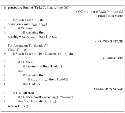
1: procedureError(hTaskiT, float, bool OC)

.OC = 1→use RAS; 0→use GS

.Error is in #tasks

2: foreach TasktinT do

t.duration = min(t.trem, t.tnew)

3: ifOCthen

4: ift.runningthen

t.saving =t.c×t.trem− (t.c+1) ×tnew

.PRUNING STAGE

SortAscending(T, “duration”)

hTaskiΓ←φ

5: foreach TasktinT[0 :T.count()(1−)]do

.Earliest tasks

6: ifOCthen

7: ift.saving>0then Γ.add(t)

8: else

9: ift.runningthen

10: ift.tnew<t.tremthen Γ.add(t)

11: elseΓ.add(t)

.SELECTION STAGE

12: if Γ_,nullthen

13: ifOCthen SortDescending(Γ, “saving”)

14: elseSortDescending(Γ, trem)

returnΓ.first()

Pseudocode 2: GS and RAS speculation algorithms for error-bound jobs (error-bound of). T is the set of unfinished tasks with the following fields per task: trem, tnew, and a boolean “running” to denote if a copy of it is currently executing. The trem of the task is the minimum of all its running copies. RAS is used when OC is set. At default, both algorithms schedule the task with the highest trem.

This again represents a “greedy” prioritization for this setting.

Despite the above change to the prioritization of which task to schedule, the form of GS and RAS remain the same as in the case of deadline-bound jobs. In particular, speculative copies are evaluated in the same manner, e.g., RAS’s criterion is still to pick the task whose speculation leads to the highest resource savings. Pseudocode 2 presents the details. The pruning stage (lines 5−11) will remove from consideration those tasks that are not the earliest to contribute to the desired error bound. The list of earliest tasks is based on the effective duration of every task, i.e., the minimum of tremand tnew. During selection (lines 12−14), GS picks the task with the highest trem while RAS picks the task with the highest saving.

(31)

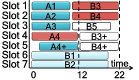
Figure 2.2: GS and RAS for error-bound job with 6 tasks. The trem and tnewvalues are when T2 finishes. The example illustrates error limit of 40% (3 tasks) and 20% (4 tasks).

tasks and 3 compute slots. The trem and tnewvalues are at 5 time units. GS decides to launch a copy of T3 as it has the highest trem. RAS conservatively avoids doing so. Consequently, when the error limit is high (say, 40%) GS is quicker, but RAS is better when the limit decreases (to, say, 20%).

2.2.2 Contrasting GS and RAS

To this point, we have seen that GS and RAS are two natural approaches for inte-grating speculation into a cluster scheduler for approximation jobs. However, the examples we have considered highlight that neither GS nor RAS is uniformly better. Natural questions to study include are these two natural approaches optimal and if they are optimal, when to apply which. In order to answer those questions and develop a better understanding of these two algorithms as well as other possible alternatives, we have developed an analytic model for speculation in approximation jobs. The model assumes wave-based scheduling and constant wave-width for a job. We present the analytic model along with formal results in the following section. The same model also inspires our design for the job-level speculation-aware cluster scheduler in Chapter 3.

2.3

Modeling and Analyzing Speculation

(32)

1 2 3 4 x 106 0

1 2 3 4

β = 1.259

order statistics

Hill estimate of

β

Figure 2.3: Hill plot of Facebook task durations.

The model focuses on a system withSslots and one job that hasT tasks₃. Each slot can have one task scheduled to it at any time. And due to the short task duration and fast processing rate, preemption is not allowed in our system. Each of the tasks has an an i.i.d. random task completion timeτ.We denote the remaining number of tasks for the job at timetbyT(t).

The key piece of our model is the characterization of the completion rate of the job, µ(t), as a function of the average number of speculative copies per task at time

t, k(t). Note that µ(t) should be interpreted as the completion rate of theith job. By focusing on the service rate we are ignoring ordering of the tasks and focusing primarily on the impact of speculation.

The statistic characteristics of the task completion time distribution have significanlt impact on the scheduler design. Our analysis of the task durations in the Facebook and Bing traces suggests that task durations have a Pareto tail (i.e., P(τ > x) =

Θ(x−β)) with shape parameterβ =1.259 as shown in the Hill plot in Figure 2.3. A Hill plot provides a more robust estimation of Pareto distributions than the, more commonly used, regression on a log-log plot [58]. To interpret the plot, a flat region corresponds to an estimate of β. The fact that the curve in Figure 2.3 is flat over a large range of order statistics (on the x-axis), but not all order statistics, indicates that the distribution of task sizes is not exactly Pareto distribution in its body, but is well-approximated by a Pareto (power-law) tail. Thus, we assume the task duration τ follows a Pareto distribution with shape parameter β and scale parameter xm in

the following discussion, where we assume the distribution is strongly heavy-tailed, i.e., 1< β ≤ 2.

In our analysis we begin with proactive speculation, and then move to reactive speculation. In proactive speculation, any task is speculated immediately to k(t)

3_{For approximation jobs,}_T _{should be interpreted as the number of tasks that are completed}

(33)

copies upon scheduling, wherek(t)is decided by the remaining number of tasksT(t)

and task completion time distribution τ. While in the reactive approach, any task is launched for a single copy at the beginning, then is speculated to k(t) copies if necessary. BesidesT(t)andτ, k(t)is also decided by the expected completion time calculated approximately by the test run of the first copy. This progression is natural since the analysis of proactive speculation serves as a stepping stone to the design of reactive speculation policies. Further, in the case of proactive speculation, we can precisely specify the optimal policy, whereas in the case of reactive speculation, we must resort to numerical optimization.

2.3.1 Proactive speculation

We start by considering a general class of proactive policies that launchk(t) specula-tive copies of tasks when the job has remaining sizeT(t). We propose the following

approximate modelfor µ(t)in this case.

µ(t)=min(S,T(t)k(t)) × E[τ]

k(t)_Emin(τ1, . . . , τ_k(t))

!

, (2.1)

whereτis a random task completion time.

To understand this approximate model, note that the first term approximates the number of slots the job occupied and the second term approximates the “blow up factor,” i.e., the ratio of the expected work completed without duplications to the amount of work done with duplications. To approximate the number of slots the job occupied, note that there areT(t)k(t)tasks available to schedule at timet, including speculative copies. Given that the maximum capacity that can be allocated isS, we obtain the first term in (2.1). The second term is the the expected amount of work done per task without speculation (E[τ]) divided by the expected amount of work done per task with speculation (k(t)E[min(τ₁, τ₂, . . . , τ_k₍_t₎)]), since k(t) copies are created and then they are stopped when the first copy completes. Perhaps the most important aspect of this approximation is the fact that task durations are i.i.d., and this is what leads both to stragglers and to the benefits of replication.

(34)

improvements in response time, especially in settings where systems are moderately or heavily loaded since improving throughput enlarges the capacity region for the system.

It is natural to follow this approach when studying stragglers because replication pushes the system toward high loads and is fundamentally about trading off increased resource demands for improved performance. Importantly, our experimental results show that the design motivated by the analysis that follows does indeed result in considerable response time improvements.

Given the model in (2.1), the question is: What proactive speculation policy max-imizes the job completion rate? As discussed above, the distribution of task sizes shows considerable evidence of a Pareto-tail, and so we focus our analysis on this setting. The following theorem states how the optimal speculation levelk(t)behaves.

Theorem 1. When task duration follows Pareto(xm,β) distribution with1< β ≤ 2,

the proactive speculation policy that maximizes the completion rate µ(t)of the job is

k(t)=    

  

2

β, S ≤ 2βT(t) S/T(t), S > 2_βT(t).

(2.2)

Proof. Under the assumption of Pareto distribution, we have,

E[τ]= βxm

β−1 E[min(τ1, . . . , τk(t)]=

kβxm

kβ−1.

(2.3)

Substitute (2.3) to (2.1),

µ(t)=     

   

k(t)β−1

k(t)2₍_β₋₁₎S, S ≤ T(t)k(t)

k(t)β−1

k(t)(β−1)T, S >T(t)k(t)

=

   

  

−(1_k − β

2) 2 S

β−1 +

β2_S

4(β−1), S ≤T(t)k(t)

(β− 1_k)_βT₋

1, S >T(t)k(t).

(35)

This theorem indicates that the optimal speculation strategy should change from conservative to aggressive as the job processes. Specifically the first line corresponds to the “early waves” and the second line corresponds to the “last wave”. During the “early waves” the optimal policy speculates conservatively corresponding to the task duration shape parameter β. In contrast, during the “last wave”, regardless of the task duration distribution, the optimal policy speculates to ensure all slots are used.

2.3.2 Reactive speculation

We now turn to reactive speculation policies, which launch copies of a task only after it has completedωwork. Both GS and RAS are examples of such policies and can be translated into choices forω. Proactive speculation is also a special case of the reactive speculation withω= 0.

Our analysis of proactive policies provides important insights into the design of reactive policies. In particular, during early waves, the the optimal proactive policy runs at most two copies of each task, and so we limit our reactive policies to this level of speculation. Additionally, the previous analysis highlights that during the last wave it is best to speculate aggressively in order to use up the full capacity, and thus it is best to speculate immediately without waitingωtime. This yields the following approximation forµ(t):

µ(t)=             

           

E[τ1]

E[τ1|0≤τ1<ω]Pr(0≤τ1<ω)+(2E[Z−ω|τ1≥ω]+ω)Pr(τ1>ω)S,

whenS ≤ T(t)(Pr(0 ≤ τ₁ < ω)+2 Pr(τ₁ ≥ ω)),

optimal proactive speculation (from (2.1)),

whenS >T(t)(Pr(0≤ τ₁ < ω)+2 Pr(τ₁ ≥ ω)),

(2.4)

whereτ1, τ2are random task durations andZ =min(τ1, τ2+ω).

Again, the first line in (2.4) approximates the completion rate during the early waves of the job, while the second line approximates the completion rate during the final wave of the job. To understand the first line, note that during early waves there are enough tasks to spawn over all the available slots S as long as

(36)

1 2 3 4 5 1

1.02 1.04 1.06 1.08 1.1

1.12 GS RAS

ω

Processing Time/Optimal

5 waves 4 waves 3 waves 2 waves 1 waves

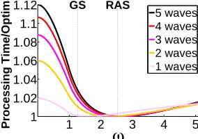
Figure 2.4: Near-optimality of GS & RAS under Pareto task durations (β= 1.259).

speculation (E[τ]) and the denominator is the expected amount of work per task with reactive speculation. This isE[τ|τ < ω]if the initial copy finishes before ω, and 2E[Z −ω|τ₁ > ω]+ωif the initial copy takes longer thanω.

Within this model, our design problem can now be reduced to finding ω that minimizes the response time of the job. GS and RAS both correspond to particular rules for how to choose ω. To see this, we can define tnew = E[τ] and trem =

E[τ − ω|τ > ω], where τ is a random task duration. Then, under GS, ω is the time when E[τ] = E[τ − ω|τ > ω], and, under RAS, ω is the time when 2E[τ] = E[τ −ω|τ > ω]. The complicated form of (2.4) makes it difficult to understand the optimalωanalytically, and thus we use numerical calculations. Figure 2.4 contrasts the performance of all the replication policies in this more general class. Specifically, it shows the ratio of the completion rates of the replication policies with parameterω normalized with respect to the optimal completion rate. It illustrates this ratio for jobs of differing numbers of waves, and forω in a wide normalized range. To highlight GS and RAS, they are shown via vertical lines. The completion rates shown in the figure are computed using the model and analysis described above. The main conclusion from this figure is neither GS or RAS is universally optimal, but each is near-optimal for jobs with a certain number of waves: RAS for jobs with large numbers of waves and GS for jobs with small numbers of waves.

2.3.3 Optimal speculation design guidelines

(37)

during the early waves of a job than during the final wave.

Guideline 1. During the early waves of a job, speculation is only valuable if task

durations are extremely heavy tailed, e.g., Pareto with infinite variance (i.e., with

shape parameterβ <2). In this case, it is optimal to speculate conservatively, using ≤2copies of a task.

This guideline is relevant because task durations are indeed heavy-tailed for the Facebook and Bing traces (see the Hill plot in Figure 2.3), which suggests that task durations have a Pareto tail (i.e., P(τ > x) = θ(x−β)) with shape parameter β = 1.259. While both GS and RAS speculate during early waves, RAS is more conservative than GS and thus outperforms it during early waves.

Guideline 2. During the final wave of a job, speculate aggressively to fully utilize

the allotted capacity.

This guideline says that, even if all tasks are currently scheduled, if a slot becomes available it should be filled with a speculative copy. While both GS and RAS do this to some extent, GS speculates more aggressively than RAS and thus, outperforms RAS during the final wave.

The previous two guidelines highlight a tradeoff between RAS and GS, which we formalize next.

Guideline 3. For jobs that require more than two waves RAS is near-optimal, while

for jobs that require fewer than two waves GS is near-optimal.

This guideline is direct conclusion from our analysis in Section 2.3.2 based on numerical optimization shown in Figure 2.4 .

2.4

_Grass

Speculation Algorithm

In this section, we build our speculation algorithm,GRASS.4Our theoretical analysis summarized in Section 2.3 motivates a design that uses RAS during the early waves of jobs and GS during the final two waves. A simplestrawmansolution to achieve this would be as follows. For deadline-bound jobs, switch from RAS to GS when the time to the deadline is sufficient for at most two waves of tasks. Similarly, for

4

(38)

error-bound jobs, switch when the number of (unique) scheduled tasks needed to satisfy the error-bound makes up two waves.

Identifying the final two waves of tasks is difficult in practice. Tasks are not scheduled at explicit wave boundaries but rather as and when slots open up. In addition, the wave-width of jobs does not stay constant but varies considerably depending on cluster utilization. Finally, task durations are varied and hard to estimate.

In light of these difficulties, we interpret the guideline as follows: RAS is better when the deadline is loose or the error limit is low, while otherwise GS performs better. This mimics the intuition from the examples in Section 2.2.1. Therefore, GRASSseeks to switch from RAS to GS as it getsclose to the job’s approximation

bound.

The complexities in these systems mean that precise estimates of the optimal switch-ing point cannot be obtained from our model. Instead, we adopt an indirect learnswitch-ing based approach where inferences are made based on executions of previous jobs (with similar number of tasks) and cluster characteristics (utilization and estimation accuracy). We compare our learning approach to the strawman described above in Section 2.6.3.

2.4.1 Learning the Switching Point

An ideal approach would accumulate enough samples of job performance (accuracy or completion time) based on switching to GS at different points. For deadline-bound jobs, this is decided by the remaining time to the deadline. For error-deadline-bound jobs, this is decided by the number of tasks to complete towards meeting the error. To speed up our sample collection, instead of accumulating samples of switching to GS, we simply generate samples of job performance using GS or RASthroughout

the job (described shortly in Section 2.4.2).

(39)

above calculation for the optimal switching point is performed periodically during the job’s execution.

For example, when a deadline-bound job has 6s of its deadline remaining,GRASS compares the potential accuracy obtained if it were to switch at each point in its future (at 1s granularity). The accuracy if it were to switch after, say, 2s is the sum of accuracies of jobs with deadlines of 2s that used only RAS and those with 4s that used only GS. Switching happens if among all such points, the best accuracy is obtained by switching now.

The size of the job alone is insufficient to calculate the optimal switching point. Even jobs of comparable size might have different numbers of waves depending on the number of available slots. Therefore, we augment our samples of job performance with the number of waves, simply approximated using currentcluster utilization. Finally, estimation accuracy of trem and tnew also decides the optimal switching point. RAS’s cautious approach of considering the opportunity cost of speculating a task is valuable when task estimates are erroneous. In fact, at low estimation accuracies (along with certain values of utilization and deadline/error-bound), it is better to not switch to GS at all and to employ RAS all along. Section 2.6.3.2 analyzes the impact of these three factors.

Therefore, GRASS obtains samples of job performance with both GS and RAS across values of deadline/error-bound, estimation accuracy of trem and tnew, and cluster utilization. It uses these three factors collectively to decide when (and if) to switch from RAS to GS. We next describe how the samples are collected.

2.4.2 Generating Samples

As described above,GRASScompares samples of job performance that use only GS or RAS throughout, to decide when to switch. These samples have to be updated continuously to stay abreast with dynamic changes in clusters. To continuously generate such samples, we introduce aperturbationinGRASS’s switching decision. With a small probabilityξ,GRASSdecides tonotswitch and instead picks one of GS or RAS for the entire duration of the job (both GS and RAS are equally probable). Such perturbation helps us obtain comparable samples.

(40)

in prior work defines an optimal value ofξby making stochastic assumptions about the distribution of the costs and the associated rewards [59]. Our setup, however, does not yield itself to such assumptions as the underlying distribution can be ar-bitrary. Another class of techniques that we considered modifiedξ with time [60]. Over time, the value of ξ is gradually reduced using a damping function, thus in-dicating higher confidence in the learned value. We decided against such damping of ξ because clusters constantly evolve with new software and hardware modules, leading to newer interactions between them.

Therefore, we pick a constant value ofξusing empirical analysis. A job is marked for generating performance samples with a probability ofξ, and we pick GS or RAS with equal probability. In practice, we bucket jobs by their number of tasks and compare only within jobs of the same bucket.

2.5

Implementation

We implement GRASSon top of two data-analytics frameworks, Hadoop (version 0.20.2) [4] and Spark (version 0.7.3) [52], representing batch jobs and interactive jobs, respectively. Hadoop jobs read data from HDFS while Spark jobs read from in-memory RDDs. Consequently, Spark tasks finished quicker than Hadoop tasks, even with the same input size. Note that while Hadoop and Spark use LATE[18] currently, we also implement Mantri[17] to use as a second baseline.

Implementing GRASS required two changes: task executors and job scheduler. Task executors were augmented to periodically report progress. We piggyback on existing update mechanisms of tasks that conveyed only their start and finish. Progress reports were configured to be sent every 5% of data read/written. The job scheduler collects these reports, maintains samples of completed tasks and jobs, and decides the switching point.

2.5.1 Task Estimators

GRASSuses two estimates for tasks: remaining duration of a running task (trem) and duration of a new copy (tnew).

(41)

Estimating tnew: We estimate the duration of a new task by sampling from durations of completed tasks (normalized to input and output sizes). The tnew values of all tasks are updated whenever a task completes.

Accuracy of estimation: While the above techniques are simple, the downside is the error in estimation. Our estimates of trem and tnew achieve moderate accuracies of 72% and 76%, respectively, on average. When a task completes, we update the accuracy using the estimated and actual durations. GRASS uses the accuracy of estimation to appropriately switch from RAS to GS.

2.5.2 DAG of Tasks

Jobs are typically composed as a DAG of tasks withinputtasks (e.g.,map or extract) reading data from the underlying storage and intermediate tasks (e.g., reduce or join) aggregating their outputs. Even in DAGs of tasks, the accuracy of the result is decided by the fraction of completed input tasks. This makesGRASS’s functioning straightforward in error-bound jobs—complete as many input tasks as required to meet the error-bound and all intermediate tasks further in the DAG.

For deadline-bound jobs, we use a widely occurring property that intermediate tasks perform similar functions across jobs. Further, they have relatively fewer stragglers. Thus, we estimate the time taken for intermediate tasks by comparing jobs of similar sizes and then subtract it to obtain the deadline for the input tasks.

Input tasks of a job, typically, read equal amounts of data. Thus, the fraction of tasks completed represents fraction of data processed too, thus making it a good indicator of the result’s accuracy.

2.6

Evaluation

We evaluate GRASS on a 200 node EC2 cluster. Our focus is on quantifying the performance improvements compared to current designs, i.e., LATE [18] and Mantri [17], and on understanding how close to the optimal performanceGRASS comes. Our main results can be summarized as follows.

(42)

Facebook Microsoft Bing Dates Oct 2012 May-Dec 2011 Framework Hadoop Dryad Script Hive [11] Scope [24] Jobs 575K 500K Cluster Size 3,500 Thousands Straggler– LATE [18] Mantri [17] mitigation

Table 2.1: Details of Facebook and Bing traces.

2. GRASS’s learning based approach for determining when to switch from RAS to GS is over 30% better than simple strawman techniques. Further, the use of all three factors discussed in Section 2.4.1 is crucial for inferring the optimal switching point. (Section 2.6.3)

2.6.1 Methodology

Workload: Our evaluation is based on traces from Facebook’s production Hadoop [4] cluster and Microsoft Bing’s production Dryad [61] cluster. The traces capture over half a million jobs running across many months (Table 2.1). The clusters run a mix of interactive and production jobs whose performance have significant impact on productivity and revenue. The jobs had diverse resource requirements of CPU, memory and IO. To create our experimental workload, we retain the inter-arrival times, input files and number of tasks of jobs. The jobs were, however, not approxi-mation queries and required all their tasks to complete. Hence, we convert the jobs to mimic deadline- and error-bound jobs as follows.

For experiments on error-bound jobs, we pick the error tolerance of the job ran-domly between 5% and 30%. This is consistent with the experimental setup in recently reported research [21, 62]. Prior work also recommends setting deadlines by calibrating task durations [21, 47]. For the purpose of calibration, we obtain the ideal duration of a job in the trace by substituting the duration of each of its task by the median task duration in the job, again, as per recent work on straggler mitigation [15]. We set the deadline to be an additional factor (randomly between 2% to 20%) on top of this ideal duration.

Job Bins: We bin jobs by their number of tasks. We use three distinctions “small” (< 50 tasks), “medium” (51−500 tasks), and “large” (> 500 tasks).

(43)

0 10 20 30 40 50

< 50 51-500 > 501 Baseline:LATE Baseline:Mantri

Job Bin (#Tasks)

Im p ro v e m e n t (% ) in A v e ra g e A c c u ra c y

(a)FB Workload–Hadoop

Job Bin (#Tasks)

Im p ro v e m e n t (% ) in A v e ra g e A c c u ra c y 0 10 20 30 40 50

(b)Bing Workload–Hadoop

0 10 20 30 40 50 60

Job Bin (#Tasks)

(c)FB Workload–Spark

Job Bin (#Tasks)

Im p ro v e m e n t (% ) in A v e ra g e J o b D u ra ti o n 0 10 20 30 40 50

(d)Bing Workload–Spark

Figure 2.5: Accuracy Improvement in deadline-bound jobs with LATE [18] and Mantri [17] as baselines.

is repeated five times and we pick the median. We measure improvement in the average accuracy for deadline-bound jobs and average duration for error-bound jobs. We also use a trace-driven simulator to evaluate at larger scales and over longer durations. The simulator replays all the task properties including their straggling. Baseline: We contrast GRASS with two state-of-the-art speculation algorithms— LATE [18] and Mantri [17].

2.6.2 Improvements fromGRASS

We contrast GRASS’s performance with that of LATE [18], Mantri [17], and the optimal scheduler.

2.6.2.1 Deadline-bound jobs

(44)

0 10 20 30 40 50

2-5 6-10 11-15 16-20 Facebook Bing

Deadline (%) Bin

(a)Deadline Bins

0 10 20 30 40

5-10 11-15 16-20 21-25 26-30

Facebook Bing

Error (%) Bin