APPLICATION OF CHEMICAL TRANSPORT MODELS TO STUDY
GLOBAL AND REGIONAL AIR QUALITY AND HUMAN HEALTH
Yuqiang Zhang
A dissertation submitted to the faculty at the University of North Carolina at Chapel Hill in partial fulfillment of the requirements for the degree of Doctor of Philosophy in the Department
of Environmental Sciences and Engineering in the Gillings School of Global Public Health.
Chapel Hill 2016
ABSTRACT
Yuqiang Zhang: Application of Chemical Transport Models to Study Global
and Regional Air Quality and Human Health
(Under the direction of J. Jason West)
Climate change and air quality are interrelated issues. Policies to mitigate greenhouse gas (GHG) emissions will not only slow climate change, but can also bring co-benefits of improved air quality and avoided mortality.
Here I examine the co-benefits of global and regional GHG mitigation on US air quality and human health in 2050 at fine resolution by dynamically downscaling a previous global study on the co-benefits of global GHG mitigation. The US average total co-benefits of global GHG mitigation in RCP4.5 are 0.47 µg m-3 for annual average PM2.5 and 3.55 ppb for ozone-season maximum daily 8-hour average O3, avoiding 24500 (90% confidence interval, 17800-31100) all-cause deaths related to PM2.5, and 12200 (5400-18900) respiratory deaths for O3. Reductions in co-emitted air pollutants dominate the total co-benefits, much higher than those via slowing climate change. GHG mitigation from foreign countries avoids 3700 (2700-4700) PM2.5-related deaths (15% of the total), and contributes more to the US O3 reduction than domestic GHG mitigation, avoiding 7600 O3-related deaths (3400-11900, 62%), highlighting the importance of global methane reductions and intercontinental air pollutant transport. GHG mitigation in the US residential sector brings the largest co-benefits for PM2.5-related deaths (21% of the total
by coordinating GHG reductions with foreign countries. Previous studies estimating co-benefits locally or regionally may greatly underestimate the full co-benefits of coordinated global actions.
ACKNOWLEDGEMENTS
I am sincerely grateful to my advisor, Dr. J Jason West, for his continual support throughout my doctoral program, for his patience, guidance and extensive knowledge. His mentorship helped me throughout my research and dissertation. His kindness and patience makes the Ph.D. process more sufferable. I am thankful for the pleasant research environment he provided for me.
Besides my advisor, I would also thank all my committee members, Dr. Will Vizuete, Dr. Jason Surratt, Dr. Jared Bowden and Dr. Chip Konrad for their insightful comments and suggestions toward improving this work, also for their hard questions which incented me to deepen my research and broaden my perspective. I especially thank Jared Bowden, who guided me on the WRF
downscaling process, and was always a good mentor and friend to me.
I also thank my fellow labmates for accompanying me on the sleepless nights we worked on environmental physics which I will never forget, for the stimulating discussions on research questions and their tremendous help on model runs. Also to all my friends in US and China, who always trusts me, believe in me and encourages me on my journey.
TABLE OF CONTENTS
LIST OF TABLES ... x
LIST OF FIGURES ... xi
LIST OF ABBREVIATIONS ... xiii
CHAPTER 1. INTRODUCTION ... 1
1.1 Air pollution as a global issue ... 2
1.2 Air pollution and premature mortality ... 4
1.3 Interactions between climate change and air quality ... 6
1.4 Dynamical downscaling ... 8
1.5 Motivations and objectives ... 9
CHAPTER 2. CO-BENEFITS OF GLOBAL AND REGIONAL GREENHOUSE GAS MITIGATION ON U.S. AIR QUALITY IN 2050 ... 12
2.1 Introduction ... 12
2.2 Methodology ... 15
2.2.1 Regional meteorology ... 17
2.2.2 Regional emissions ... 19
2.2.3 Regional air quality model and dynamical chemical BCs ... 21
2.2.4 Scenarios ... 22
2.3.1 CMAQ model evaluation ... 23
2.3.2 Air quality changes in 2050 ... 25
2.3.3 Total co-benefits for U.S. air quality from global GHG mitigation ... 26
2.3.4 Co-benefits from the two mechanisms ... 27
2.3.5 Co-benefits from domestic and foreign GHG mitigation ... 28
2.3.6 Regional co-benefits and variability... 29
2.4 Discussion ... 30
2.5 Conclusions ... 32
2.6 Figures and Tables ... 34
CHAPTER 3. CO-BENEFITS OF GLOBAL, DOMESTIC, AND SECTORAL GREENHOUSE GAS MITIGATION ON US AIR POLLUTION AND HUMAN HEALTH IN 2050 ... 45
3.1 Introduction ... 45
3.2 Methods ... 48
3.2.1 Air quality changes in US in 2050 at fine scale ... 48
3.2.2 Human health analysis ... 49
3.3. Results and discussion ... 51
3.4 Conclusions ... 55
3.5 Figures and Tables ... 57
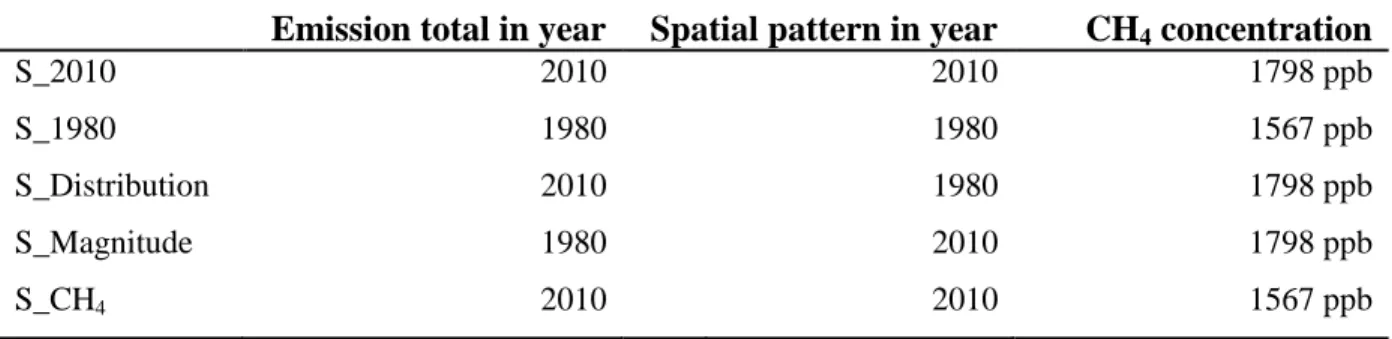
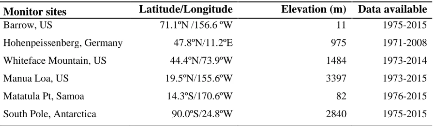
CHAPTER 4. SOUTHWARD REDISTRIBUTION OF EMISSIONS DOMINATES THE 1980 TO 2010 TROPOSPHERIC OZONE CHANGE ... 64
4.2 Methods ... 66
4.2.1 Global emissions spatial pattern change ... 66
4.2.2 CAM-chem model configuration ... 67
4.2.3 CAM-chem evaluation ... 68
4.2.4 Data sources ... 69
4.2.5 Code availability ... 70
4.3 Discussions and Results ... 70
4.4 Conclusions ... 74
4.5 Figures and Tables ... 76
CHAPTER 5. CONCLUDINGS REMARKS ... 82
5.1 Key scientific findings ... 82
5.1.1 Co-benefits from GHG mitigation ... 82
5.1.2 Emission pattern redistribution on global ozone burden ... 86
5.2 Policy implications ... 87
5.3 Uncertainties and future research ... 88
APPENDIX A. CO-BENEFITS OF GLOBAL AND REGIONAL GREENHOUSE GAS MITIGATION ON U.S. AIR QUALITY IN 2050: SUPPORTING MATERIALS ... 93
APPENDIX B. CO-BENEFITS OF GLOBAL, DOMESTIC, AND SECTORAL GREENHOUSE GAS MITIGATION ON US AIR QUALITY AND HUMAN HEALTH IN 2050: SUPPORtING MATERIALS ... 120
APPENDIX D. GUIDE TO RUNNING CAM-CHEM MODEL
LIST OF TABLES
Table 2. 1. List of CMAQv5.0.1 simulations in this study. Hourly BCs are from the MOZART-4 (MZ4) simulations of WEST2013. We fix the methane (CH4) background
concentrations in CMAQ consistent with the RCP scenarios and WEST2013. ... 34 Table 2. 2. Anthropogenic emissions in the U.S. for major air pollutants in 2000 and 2050 from REF and RCP4.5 (Tg yr-1), and the relative differences (Relative Diff) between RCP4.5 and REF in 2050 ((RCP4.5 - REF)/REF×100). ... 35 Table 2. 3. Evaluation of the S_2000 simulation (average of three years modeled) with surface observations in 2000 for PM2.5 (µg m-3) and O3 (ppb) ... 36 Table 3. 1. Co-benefits for air quality changes in the US in 2050 from global,
domestic and sectoral GHG mitigation. For PM2.5 (µg m-3) we use three-year averages,
and for O3 (ppbv), we calculate the 6-month ozone season of 1-hr daily maximum, and then average over three years………..57
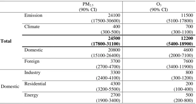
Table 3. 2. Estimated total co-benefits for avoided premature mortality in 2050
from PM2.5-related all-cause mortality and O3-related respiratory mortality. The values in the brackets are 90% confidence intervals (CI). ... 58
LIST OF FIGURES
Fig. 2. 1. Changes in (a) 2-m temperature (°C) and (b) precipitation (mm/day) centered on 2050 between RCP8.5and RCP4.5 (RCP8.5—RCP4.5). ... 37 Fig. 2. 2. Comparison of annual U.S. average concentration changes for RCP4.5 in 2050 relative to 2000, for this study (black triangle), MZ4 from WEST2013 (red circle), and the ensemble mean (blue diamond) and multi-model range from ACCMIP (blue lines), for (a) PM2.5, and (b) O3. In panel a, the total PM2.5 reported by the ACCMIP models is shown on the left, and the PM2.5 estimated as a sum of species
BC+OA+SOA+SO4+NO3+NH4+0.25*SeaSalt+0.1*Dust following Fiore et al. (2012) and Silva et al. (2013) shown on the right. Values shown are the average of three years for CMAQ and MZ4, and 5 to 10 years for ACCMIP
for three models (LMDzORINCA, GFDL-AM3 and GISS-E2-R) that report O3 and two models (GFDL-AM3 and GISS-E2-R) that report PM2.5. ... 38
Fig. 2. 3. The three-year averages PM2.5 (µg m-3) distributions in 2050 from (a) S_REF, (b) S_RCP45, and (c) the total co-benefits (shown as the difference between S_RCP45 and S_REF). Blue colors in panel (c) indicate an air quality improvement. ... 39 Fig. 2. 4. Seasonal distributions of total co-benefits for PM2.5 (µg m-3) for (a) winter, (b) spring, (c) summer and (d) fall.. ... 40 Fig. 2. 5. The three-year ozone-season averages (May to October) of MDA8 O3 (ppb) from (a) S_ REF, (b) S_ RCP45, and (c) the total co-benefits (shown as the difference
between S_RCP45 and S_REF). Blue colors in panel (c) indicate an air quality improvement. ... 41 Fig. 2. 6. Benefits of reduced co-emitted air pollutants (a, b) versus slowing climate change (c,d) for PM2.5 (a, c) and ozone season MDA8 surface O3 (b, d). Blue colors indicate an air quality improvement. The numbers on the plots are three-year averages of air quality changes over the U.S. ... 42 Fig. 2. 7. Benefits of domestic (a,b) versus foreign (c,d) GHG reductions for PM2.5 (a, c) and ozone season MDA8 surface O3 (b, d). Blue colors indicate an air quality improvement. The numbers on the plots are three-year averages of air quality changes over the U.S. ... 43 Fig. 2. 8. Mean values of domestic (blue) and foreign co-benefits (red) for U.S. average (a) annual PM2.5, and (b) ozone season MDA8 O3. The numbers below each bar are the percentage (%) of the foreign co-benefit. ... 44 Fig. 3. 1. Total air quality co-benefits in 2050 for (a) annual average PM2.5, and
Fig. 3. 2. Total co-benefits (S_RCP45-S_REF) for avoided premature mortality (deaths yr-1) for (a) PM2.5 (all-cause mortality), and (b) O3 (respiratory mortality) in US in 2050. Total avoided deaths and 90% confidence intervals are shown at the top of each panel. ... 60 Fig. 3. 3. Comparisons between this study (red) and WEST2013 (blue) of the avoided human mortality (1000 deaths yr-1) from air quality changes in 2050 compared with 2000, for (a) REF scenario, (b) RCP4.5 scenario, and (c) the total co-benefits in 2050. The red lines represent the 90% confidence intervals (CI) for this study, and blue lines are 95% CI for WEST2013. RESP indicates for the mortality from O3-related respiratory deaths, CPD for PM2.5-related cardiopulmonary deaths, and LC for PM2.5-related lung cancer. ... 61 Fig. 3. 4. The emission co-benefits (a, b) and climate co-benefits (c, d) for avoided
human mortality (deaths yr-1) from PM2.5 (a, c)and O3 (b, d). White in panels c and d indicates increased mortality attributed to slowing climate change, from increases in air pollutant concentrations. Total avoided deaths and 90% confidence intervals are shown at the top of each panel. ... 62 Fig. 3. 5. The domestic co-benefits (a, b) and foreign co-benefits (c, d) for avoided all-cause mortality from PM2.5 (a, c) and respiratorymortality from O3 (b, d) in US in 2050. Total avoided deaths and 90% confidence intervals are shown at the top of each panel. ... 63 Fig. 4. 1. Tropospheric O3 burden change (
∆
B
O3) from 1980 to 2010. a, For global,NH and SH. b, For different latitudinal bands. The estimated components for
3 O
B
∆
due to the spatial pattern change (red rectangle), magnitude change (black triangle) and global CH4 change (purple circle) are also seen in each plot………80
Fig. 4. 2. Spatial distributions for
3 O
B
LIST OF ABBREVIATIONS
ACCMIP Atmospheric Chemistry and Climate Model Intercomparison Project
ACS American Cancer Society
AE6 Aerosol 6 Module
AF Attributable Fraction
AM3 NOAA GFDL Atmospheric Model Component of CM3
AMWG Atmosphere Model Working Group
AQS Air Quality System
BC Black Carbon
BCs Boundary Conditions
BenMAP-CE Benefits Mapping and Analysis Program-Community Edition BEIS Biogenic Emission Inventory System
ΔBO3 Change in tropospheric ozone burden
BO3 Tropospheric ozone burden
BVOC Biogenic Volatile Organic Compound
CA California
CAM-Chem Community Atmosphere Model with Chemistry CASTNET Clean Air Status and Trends Network
CB05 Chemical Bond 2005
CESM Community Earth System Model
CI Confidence Interval
Cl- Chloride
CMAQ Community Multi-scale Air Quality
CO Carbon Monoxide
CO2 Carbon dioxide
CONUS CONtiguous United States
CPD Cardiopulmonary disease
CRF Concentration Response Function CSN Chemical Speciation Network CTMs Chemical Transport Models
CV Coefficient of Variation
DU Dobson Unit
EC Elemental Carbon
ENE Energy
EPA Environmental Protection Agency
GCAM Global Change Assessment Model
GCMs General Circulation Models
GDP Gross Domestic Product
GEOS-5 The Goddard Earth Observing System Model, Version 5 GFDL Geophysical Fluid Dynamics Laboratory
GHG Greenhouse gas
HIF Health Impact Function
hPa hectopascal
IC Initial Condition
IMPROVE Interagency Monitoring of PROtected Visual Environments
IND Industry
IPCC Intergovernmental Panel on Climate Change ISOPNO3 peroxy radical from NO3+ isoprene
Km Kilometer
LC Lung cancer
LO3 ozone chemical loss rate
MEGAN Model of Emissions of Gases and Aerosols from Nature MCIP Meteorology-Chemistry Interface Processor
MDA8 Maximum Daily 8-hour Average
MdnB Median Bias
MdnE Median Error
MOZART-4 Model for OZone And Related chemical Tracers, version 4 MPAN methacryloyl peroxynitrate
µg m-3 Micrograms per cubic meter
°N Degrees North
Na+ Sodium
NAAQS National Ambient Air Quality Standards
NASA National Aeronautics and Space Administration
NEI National Emission Inventory
NH4+ Ammonium
NH North Hemisphere
NMdnB Normalized Median Bias
NMdnE Normalized Median Error
NMVOCs Non-Methane Volatile Organic Compounds NOAA National Oceanic and Atmospheric Administration
NO nitrogen monoxide
NO2 nitrogen dioxide
NO3- Nitrate
NOx Nitrogen oxides
NOy total reactive nitrogen N2O5 Dinitrogen pentoxide
NY New York state
O3 Ozone
OA Organic Aerosol
OC Organic Carbon
OM Organic Matter
OMI Ozone Monitoring Instrument OPE Ozone Production Efficiency
PAN Peroxyacyl nitrates
PI Posterior interval
PMC Particulate Matter Coarse
PM2.5 Particles with aerodynamic diameters of 2.5 µm or less
PO3 ozone chemical production rate
Pop Exposed population
ppbv Parts per billion by volume RCMs Regional Climate Models
RCP Representative Concentration Pathway RCP4.5 Representative Concentration Pathway 4.5 RCP8.5 Representative Concentration Pathway 8.5
REF REFerence
Res Respiratory disease
RES Residential
RETRO Reanalysis of the Tropospheric Chemical Composition over the past 40 years
RF Radiative Forcing
RR Relative Risk
°S Degrees South
SCC Source Clarification Codes
SH South Hemisphere
SMOKE Sparse Matrix Operator Kernel Emissions
SIP State Implementation Plans
SOA Secondary organic aerosol
Tg Teragram
TX Texas
US United States of America
UTC Coordinated Universal Time VOCs Volatile organic compounds
WACCM Whole Atmosphere Community Climate Model WEST2013 West et al., 2013
WHO World Health Organization W m-2 Watts per square meter
CHAPTER 1. INTRODUCTION
The 20th century was a rapid changing period, featured with increasing of global
population from 1.7 billion to 6.1 billion (United Nations, 2001), global gross domestic product (GDP) by 19 times (International Monetary Fund, 2000), and fossil fuel consumption by 15 times (Smil, 2003). Air pollution is among one of the top issues raised by this unprecedented change. Clean air is a basic requirement for human health, crop yield and ecosystems (Royal Society, 2008). A recent study attributed the global deaths and disability-adjusted life years in 2010 to 67 risk factors using global scale modeling (Lim et al., 2013), and found that three risk factors in the category of “Air Pollution” have important health impacts: ambient particulate matter pollution (attributing 3.2±0.4 million deaths in 2010), household air pollution from solid fuels (3.5 million deaths, ranging from 2.7 to 4.4 million) and ambient ozone pollution (0.2 million deaths, ranging from 0.1 to 0.3 million). Fine particulate matter (PM2.5, particles with aerodynamic diameter of 2.5 µm or less) and ozone (O3) therefore directly link air quality and human health impacts.
atmosphere. For O3 in the troposphere, it is secondary air pollutant, mainly produced by photochemical reactions of CO, non-methane volatile organic compounds (NMVOCs), and methane (CH4) in the presence of NOx and sunlight. Tropospheric O3 can also be transported from stratosphere through the stratosphere-troposphere-exchange (STE), but this is less important than chemical production (Young et al., 2013).
1.1 Air pollution as a global issue
Despite a relatively short lifetime in the atmosphere (days to weeks), PM2.5 and its precursors can be transported long-distance from source region to another reception region (Ewing et al., 2010; Hadley et al., 2007; Han et al., 2008; Heald et al., 2006; Kondo et al., 2011; Liu et al., 2009a, b; Nam et al., 2010; TF HTAP, 2010; Wuebbles et al., 2007; Yu et al., 2012; Yumimoto et al., 2010). For example, Liu et al. (2009a) found that the influence from
dominating the premature mortality from outdoor pollution, compared with O3 (Anenberg et al., 2010; Lim et al., 2013; Silva et al., 2013). So both PM2.5 and O3 are increasingly recognized as a global issue instead of regional one, demanding more international collaborations (Holloway et al., 2003; Keating et al., 2004; TF HTAP, 2010).
To control outdoor air pollution on national scale, strict standards should be made to reduce the air pollutants emissions from domestic emissions sectors, such as power plants, cement industry and ground transportation (e.g., the State Implementation Plans, a.k.a., SIP in US; Wang et al., 2012, 2014). On international scale, close collaborations should be established to keep the air pollutants global background levels from increasing, and to help reach individual goal of the air quality standards for concerned countries. The air pollutants in the North
Hemisphere (NH) can be transported from East Asia to North America, from North America across the North Atlantic Ocean to Europe, and from Europe into the Arctic and East Asia. Studies have shown that the global O3 burdens are more sensitive to the air pollutants changes in the tropical regionals and the South Hemisphere (SH) (Berntsen et al., 2005; Derwent et al., 2008; Fuglestvedt et al., 1999, 2010; Fry et al., 2012, 2014; Naik et al., 2005; West et al., 2009a). So to control PM2.5 and O3 as both a global and regional issue, not only the magnitude of emissions of the air pollutants and its precursors should be considered, but also where these emissions should be reduced.
The concentrations and the distributions of the air pollutants in the atmosphere are
Atmospheric chemical transport models (CTMs) are great tools to study the large-scale or continental-scale air pollutants distributions and transport. The CTMs are designed to calculate and predict the chemical reactions, physical processes and the transport of the air pollutants within the atmosphere. Since monitor sites, including ground surface observations, balloons and satellites, cannot provide complete spatial and temporal coverage for the interest of domain, under these circumstances, CTMs are widely used in global and regional studies for regulatory or policy assessment, understanding chemical and physical processes, source attribution, and health impact assessments. More recently, the CTMs are used heavily to predict future air quality changes under future climate change of different projections.
1.2 Air pollution and premature mortality
A larger number of epidemiological studies have quantified the relationship between adverse health effects with PM2.5 (Dockery et al., 1993; Laden et al., 2006; Krewski et al., 2009; Roman et al., 2008) and O3 (Bell et al., 2004, 2005; Jerrett et al., 2009; Levy et al., 2005). An early study was the 1993 Harvard Six Cities study, which found associations between expose to PM2.5 and lung cancer and cardiopulmonary mortality (Dockery et al., 1993). An extended follow-up study was performed later with 8 more years’ data to study the reduced mortality from the reduced PM2.5 pollution (Laden et al., 2006). Reduced mortality risks were associated with reduced ambient PM2.5 concentrations, reaffirming the associations between the PM2.5 and the mortality. In this latest cohort study, the relative risks (RR) for total all-cause mortality, lung cancer and the cardiovascular deaths were 1.16 (with a 95% confidence interval, CI of 1.07-1.26), 1.27 (95% CI, 0.96-1.69), and 1.28 (95% CI, 1.13-1.44), with each 10 µg/m3 increases in
An extended follow-up and spatial analysis of the American Cancer Society (ACS) study was also conducted to examine the association between the long-term exposure of ambient PM2.5 pollution and mortality in major large US cities (Krewski et al., 2009). This is the largest cohort study so far, involving approximately 1.2 million participants across many US large cities, and also applying state-of-art statistical approaches. This study confirmed strong associations
between the ambient PM2.5 and mortality as shown in previous studies, and also established new relationships for the RRs of the total all-cause, cardiopulmonary disease and lung cancer
mortality, with 1.06 (95% CI, 1.04-1.08), 1.13 (95% CI, 1.10-1.16), and 1.14 (95% CI, 1.06-1.23) individually (Krewski et al., 2009). The RRs from the ACS study are lower than the estimates from the Harvard Six City studies.
Studies have shown that different components of PM2.5 may have different associations with mortality, for example, the ambient black carbon (BC) may have stronger association with mortality than other components and PM as a whole (Adar et al., 2007; Bell et al., 2009; Janssen et al., 2011, 2012; Ostro et al., 2007; Peng et al., 2009; Power et al., 2011; Qiao et al., 2014; Suh et al., 2010; WHO, 2012; Wilker et al., 2013). However, a recent review by the US EPA (2010) revealed that the differences in the mortality risks associated with long-term exposure to PM2.5 components were not discernable. Studies that assess premature mortality associated with PM2.5 overwhelmingly use PM2.5 as an indicator, rather than different species.
0.31%-0.98%) (Bell et al., 2004). Moreover, surface ozone exposure is also associated with the chronic mortality. A recent long-term large-scale study cohort of the American Cancer Society Cancer Prevention Study is the first to establish the association between the long-term ozone exposure and mortality (Jerrett et al., 2009). Using the two-pollutant model, the authors found strong associations with the risk from respiratory causes, and the estimated RR was 1.40 (95% CI, 1.010-1.040) with a 10-ppb increases for the ozone season of 1-hour daily maximum O3 concentrations.
1.3 Interactions between climate change and air quality
Climate change and air quality are interrelated issues, suggesting that these two should be considered together under the mitigation strategies (Ramanathan and Feng, 2009). First, air pollutants can cause climate forcing. For example, O3 in the troposphere can warm the earth, while aerosols, such as NO3- and SO42-, two very important components of PM2.5, can cool the atmosphere by reflecting the sunlight back into the space.
quality and greater human health risk exposure in the future. Variations of temperature, water vapor and concentration of CO2 from climate change could also affect the natural biogenic emissions, which are shown to be very important in the formation of PM2.5 and O3 in rural sites (Fiore et al., 2011; Koo et al., 2010; Lam et al., 2011; Pun et al., 2002; Wiedinmyer et al., 2006).
Previous studies have used both global and regional CTMs to study the single or combined changes in future climate and emissions on global and regional air quality (Weaver et al., 2009; Jacob and Winner, 2009; Fiore et al., 2012). Climate change is likely to decrease background O3 over remote places due to the elevated humidity, and increase O3 over urban and polluted areas, in part because of higher temperature (Jacob and Winner, 2009). However, the role of climate change on PM2.5 is less clear as different components of PM2.5 may respond differently to
changes in climate variables (Jacob and Winner, 2009; Tai et al., 2010; Fiore et al., 2012, 2015). Third, the sources of emissions of greenhouse gases (GHGs) and air pollutants are usually shared (Haines et al., 2009; Nemet et al., 2010; Ramanathan and Feng, 2009; Reynolds and Kandlikar, 2008; West et al., 2004). In particular, the combustion of fossil fuels is the major source for both GHGs and air pollutants. Actions to control one can also influence the other. So the climate policies to reduce the GHGs will not only get the benefits of slowing climate change, but can also have the co-benefits of improved air quality and then human health (Bell et al., 2008; Cifuentes et al., 2001; Driscoll et al., 2015; Garcia-Menendez et al., 2015; Jacobson, 2001;
1.4 Dynamical downscaling
To study the future air quality changes under the changing climate at regional scale at fine resolution, dynamical downscaling is usually adopted to provide high quality input data for the regional CTMs. Dynamical meteorological downscaling refers to the process of taking global climate change responses from global General Circulation Models (GCMs) and translating them to a finer temporal and spatial scale which are more meaningful in the context of local and regional impacts by using the Regional Climate Models (RCMs) with the lateral boundary conditions provided from the GCMs. GCMs are used to study Earth’s climate system and simulate the future climate change. RCMs are used to simulate the climate change for a limited area at much higher spatial resolutions. The advantages of the dynamical meteorological downscaling are that a regional model can simulate local fine-scale feedback processes better than the GCMs. The disadvantages are that it requires more computational resources and the performances of the regional climate depend strictly on the input data and physical
configurations of the RCMs. The meteorological downscaling has been broadly used in previous research to study the future regional climate change under different emission projections
RCMs will not be realized. A delicate balance is needed between the amount of constraint given to the RCM and the freedom of the RCM to simulate its own mesoscale features (Otte et al., 2012).
Chemical downscaling refers to the process that simulating global perturbations in global CTMs to provide initial and boundary conditions (BCs) for regional CTMs at greater resolution in a region of interest. The proper chemical BCs are also crucial for the regional CTMs as the effects of intercontinental transport of air pollutants (Lam et al., 2009; Lin et al., 2008) and enhancement of background pollutant concentrations emerged (Fiore et al., 2003). Numerous studies implied that providing dynamical chemical BCs for the regional CTMs instead of the profiles would best capturing the temporal and spatial variations distributions of air pollutants in the regions (Byun et al., 2004; Fu et al., 2008; Tang et al., 2007). Song et al. (2008) compared the performances of CMAQ simulating vertical ozone profile by using profile BCs and
dynamical BCs, and found that dynamical BCs performed better than the scenarios with profile BCs. By providing dynamical BCs for the regional CTMs, we have the ability to consider global changes in air pollutants in the global CTMs, while simulating the effects on a finer scale at a region of interest. It will also allow us to consider the intercontinental transport of air pollutants as well as the global climate change on the influence of regional air quality.
1.5 Motivations and objectives
Recent studies also estimated the future regional GHG mitigation scenarios on the co-benefits of air quality and human health (Thompson et al., 2014; Trail et al., 2015).
However, these studies may underestimate the true co-benefits as they do not consider GHG mitigation from the whole world: GHG mitigation as a whole may slow global climate change significantly, which then could decrease the air pollutants. GHG mitigation could bring air quality improvement for those countries who participate, and can also affect air quality in the adjacent countries due to long-range air pollutant transport, especially for O3, even though those countries will not or delay participating in the mitigation policies. Under this circumstance, a recent study led by Dr. J. Jason West from UNC, which I was also involved, used a global CTM to study the global GHG mitigation on future air quality and human health (West et al., 2013). This is the first study to consider the global air quality and human health benefits by assuming all countries participate in the mitigation strategies. By using the global CTM, this study is also the first to consider the influence of global air pollution transport and long-term influences via global CH4. This study concluded that global GHG mitigation could bring significant air quality
improvement for both PM2.5 and O3, and avoid 2.2±0.8 million premature deaths globally by 2100 due to the improved air quality; it also found that when monetized, the global average marginal co-benefits of avoided mortality were $50–380/tCO2, higher than the previous estimates (Nemet et al., 2010).
the global co-benefits study. By embedding this fine-resolution regional co-benefits study into a consistent global context, I can also quantify the co-benefits from domestic GHG mitigation versus the contributions from foreign countries reductions, which has never done before. In Chapter 2, I discuss the co-benefits of global and regional greenhouse gas mitigation on U.S. air quality in 2050 (Zhang et al., 2016a). In Chapter 3, I quantify the co-benefits of global, domestic, and sectoral greenhouse gas mitigation on US air pollution and human health in 2050 (Zhang et al., 2016b).
A second motivation for my Ph.D. work is to study the global emission redistribution on the influence of global ozone burden. Since 1980, anthropogenic emissions of ozone precursors have decreased in developed regions such as North America and Europe, but increased in developing regions, particularly East and South Asia, redistributing the emissions southwards (Granier et al, 2011; Lamarque et al., 2010; Ohara et al., 2007; Richter et al., 2005; van der A et al., 2008). Modeling studies have shown that the tropospheric ozone burden and resulting radiative forcing are much more sensitive to emission changes in the tropics and Southern Hemisphere than other regions (Naik et al., 2005; West et al., 2009a; Fry et al., 2012, 2014). However, the effect of the spatial redistribution of emissions has not been isolated. In Chapter 4, I investigate the influence of the change in global emissions shifting southwards on the global tropospheric O3 burden and surface air quality from 1980 to 2010, and then compare this influence with those from the changes in global emissions magnitude and global CH4
CHAPTER 2. CO-BENEFITS OF GLOBAL AND REGIONAL GREENHOUSE GAS MITIGATION ON U.S. AIR QUALITY IN 2050
(Yuqiang Zhang, Jared H. Bowden, Zachariah Adelman, Vaishali Naik, Larry W. Horowitz, Steven J. Smith, J. Jason West. Submitted to Atmospheric Chemistry and Physics)
2.1 Introduction
Climate change and air quality are interrelated problems. First, climate change can affect the formation, destruction and transport of major air pollutants, through changes in
meteorological variables of temperature, precipitation, air stagnation events, etc. (Weaver et al., 2009; Jacob and Winner, 2009; Fiore et al., 2012, 2015). It can also affect natural emissions (biogenic, dust, fire and lighting) that influence air quality. Second, air pollutants such as particulate matter (PM) and ozone (O3) can change the climate by altering the solar and terrestrial radiation balance through direct and indirect effects (Myhre et al., 2013). Third, the sources of emissions of greenhouse gases (GHGs) and air pollutants are usually shared,
particularly through the combustion of fossil fuels, so actions to control one can also influence emissions of the other. Policies to control GHG emissions will therefore not only slow climate change in the future, but will also provide co-benefits of improvements to air quality and consequently to human health (Bell et al., 2008; Nemet et al., 2010).
elevated humidity, and increase O3 over urban and polluted areas, in part because of higher temperature. Jacob and Winner (2009) concluded that future climate change could increase summertime O3 by 1-10 ppb over polluted regions in the U.S. in scenarios from the Special Report on Emission Scenarios (SRES; Nakicenovic and Swart, 2000). In one study, climate change in 2050 under the SRES A1B scenario is projected to increase summertime O3 by 2-5 ppb over large areas in the U.S., comparable to the effect of reduced anthropogenic emissions which reduces O3 by 2-15 ppb, especially in the east (Wu et al., 2008). The overall effect of climate change on PM is less clear, as different components of PM may respond differently to changes in climate variables (Jacob and Winner, 2009; Tai et al., 2010; Fiore et al., 2012, 2015).
Many studies have also estimated the co-benefits of regional or local GHG mitigation on air quality and human health through reductions in co-emitted air pollutants. Cifuentes et al. (2001) found that GHG mitigation through reduced fossil fuel combustion could bring significant local air pollution-related health benefits to some megacities. These health benefits have been estimated in many studies (Bell et al., 2008), and give co-benefits ranging from $2-196 /tCO2 when monetized, comparable to the costs of GHG reductions (Nemet et al., 2010). A few studies also analyze the co-benefits on future air quality and human health from future regional GHG mitigation scenarios (Thompson et al., 2014; Trail et al., 2015). Thompson et al. (2014) studied the co-benefits of different U.S. climate policies on 2030 domestic air quality, and found that when monetized, the human health benefits due to the improved air quality can offset 26-1050% of the cost of the carbon polices, depending on the policy.
mitigation are relevant as meaningful GHG mitigation requires participation from at least several of the most highly-emitting nations. We examined the co-benefits of global GHG reductions on both global and regional air quality and human health, using a global atmospheric model (Model for OZone And Related chemical Tracers, version 4, MOZART-4, hereafter referred to as MZ4) and self-consistent future scenarios (West et al., 2013, referenced hereafter as WEST2013). In addition to evaluating co-benefits through reductions in co-emitted air pollutants, WEST2013 was the first study to quantify co-benefits through a second mechanism: slowing climate change and its effects on air quality. There are several other innovations of WEST2013: we account for global air pollution transport and long-term influences of methane using the global CTM; we consider realistic scenarios in which air pollutant emissions, demographics, and economic valuation are modeled consistently; and we evaluate chronic mortality influences of fine PM (PM2.5, PM with diameter smaller than 2.5 µm) as well as O3. WEST2013 concluded that global GHG mitigation could bring significant air quality improvement for both PM2.5 and O3, and avoid 2.2±0.8 million premature deaths globally by 2100 due to the improved air quality. When monetized, the global average marginal co-benefits of avoided mortality were $50–380/tCO2, higher than the previous estimates (Nemet et al., 2010). The co-benefits from the first
mechanism of reduced emitted air pollutants were shown to be much greater than the co-benefits from the second mechanism via slowing climate change.
The WEST2013 study is limited by the coarse resolution of the CTM used (2º×2.5º
decision-making for both climate change and air quality. We use a comprehensive modeling framework in the downscaling process, including a regional climate model to dynamically downscale the global climate to the contiguous United States (CONUS), an emissions processing program to directly process the global anthropogenic emissions to the regional scale, and we create dynamical boundary conditions (BCs) from the global co-benefits outputs for the regional CTM. We quantify the total co-benefits of global GHG mitigation on U.S. air quality for both PM2.5 and O3, and then separate the co-benefits from the two mechanisms analyzed by
WEST2013. We also quantify the benefits from domestic GHG mitigation versus the co-benefits from those of foreign countries’ reductions. We then present the co-co-benefits from global and domestic GHG mitigation on nine U.S. regions.
With regard to previous studies on the effect of climate change on future air quality (e.g. Jacob and Winner, 2009), our work differs in our reframing of this impact as a co-benefit of slowing climate change from GHG mitigation, and by analyzing that co-benefit through realistic future scenarios, following WEST2013. With regard to previous co-benefits studies that have been conducted on a regional scale (e.g., Thompson et al., 2014), this research differs by
embedding the regional co-benefits study in consistent global context, accounting for the effects of changes in global air pollutant emissions and climate change on U.S. air quality.
2.2 Methodology
Future air quality changes under global and regional GHG mitigation scenarios are simulated using a regional CTM. The scenarios modeled here are built on those of WEST2013, who compared the Representative Concentration Pathway 4.5 (RCP4.5) scenario with its
(Thomson et al., 2011). RCP4.5 was developed based on REF by applying a global carbon price to all world regions and all sectors including carbon in terrestrial systems. As discussed by van Vuuren et al. (2011), the air pollutant emissions for the four RCP scenarios were prepared by different groups using different models and assumptions, so they are inconsistent with one another. But by comparing REF with RCP4.5, we use a self-consistent pair of scenarios, where the difference is uniquely attributed to a climate policy. WEST2013 used both emissions and meteorology from RCP4.5 to simulate future air quality under the RCP4.5 climate policy, and used emissions from REF and meteorology from RCP8.5 to simulate future air quality assuming no climate policy. Since no General Circulation Model (GCM) conducted future climate
simulations for the REF scenario, RCP8.5 is used as a proxy for the future climate under REF. The differences between these two scenarios give the total co-benefits for future air quality under climate policy from RCP4.5. Through one extra simulation with emissions from RCP4.5 together with RCP8.5 meteorology (e45m85 in Table 2.1), and by comparing with REF and RCP4.5, WEST2013 separated the total co-benefits into the two mechanisms: the co-benefits from reductions in co-emitted air pollutants, and co-benefits from slowing climate change and its influence on air quality.
for the regional CTM. The latest version of the Community Multi-scale Air Quality model (CMAQ, v5.0.1, Byun and Schere, 2006) is used as the regional CTM to simulate air quality changes over the CONUS domain. WEST2013 simulated five consecutive years for each scenario, and used the last four years’ average for the data analysis with the first year as a spin-up. Due to the limitations of computational resources, we run CMAQ for 40 months
consecutively for each scenario, with the first 4 months as spin-up, and analyze the results as three-year averages.
2.2.1 Regional meteorology
al. (2012) and Bowden et al. (2012, 2013) demonstrated that using nudging in WRF improves the overall accuracy of the simulated climate over the CONUS at 36-km and does not squelch
extremes in temperature and precipitation. In particular, spectral nudging affects the model solution through a nonphysical term in the prognostic equations based on the difference between the spectral decomposition of the model solution and the reference analysis. Spectral nudging is used to constrain WRF toward synoptic-scale wavelengths resolved by GFDL AM3 exceeding 1200 km. Nudging is applied equally to potential temperature, wind, and geopotential with a nudging coefficient of 1.0×10⁻⁴, which is equivalent to a time scale of 2.8 hours. The downscaled meteorology from WRF is used to provide meteorological inputs to CMAQ. Hourly WRF outputs are processed using Meteorology-Chemistry Interface Processor (MCIP v4.1; Otte and Pleim, 2010) to provide meteorological inputs for CMAQ.
Comparing the downscaling results between WRF with the GFDL AM3 simulation for three-year averages of the 2-m temperature (we present three-year averages instead of four to be consistent with CMAQ outputs below), we see that the large-scale spatial patterns for
temperature are similar (Fig. A.1). However, the downscaling clearly improves the resolved features related to topography and provides a different realization of average regional climate throughout the CONUS. Comparing WRF future projected change centered on 2050 with 2000, we see that the three-year average of 2-m temperature generally increases over the entire U.S. for both RCP8.5 and RCP4.5 (Fig. A.2-A.3). Temperature increases are largest for extreme
(RCP8.5 minus RCP4.5), Fig. 2.1 illustrates that temperature increases are smaller in RCP4.5 throughout the CONUS, except in the Northwest. The precipitation difference between scenarios has a larger spatial variability than the 2-m temperature. However, the only region where the regional climate is warmer and drier in RCP4.5 is in the Northwest U.S. Ignoring other
influences of climate change, increases in precipitation would be expected to increase PM wet scavenging, and decrease PM concentration.
2.2.2 Regional emissions
Similar studies in the past have typically chosen to run SMOKE with the present-day U.S. National Emission Inventory (NEI), and then scale the SMOKE outputs into future years, using the mass ratio of projected future to present-day emissions from global inventories (e.g., Hogrefe et al., 2004; Nolte et al., 2008; Avise et al., 2009; Chen et al., 2009; Gao et al., 2013). Instead, we use SMOKE to directly process the global emissions in 2000 and in 2050 from REF and RCP4.5 to provide temporally- and spatially-resolved CMAQ emission input files. We first regrid the global emissions datasets at 0.5º×0.5º into finer resolution (36km×36km), and then take advantage of the temporal and speciation profiles inside SMOKE to assign temporal variations and re-speciate the PM and VOCs species. By doing this, we account better for the spatial distribution changes of future emissions projected in the RCPs (Fig. S4-S10), whereas the traditional method only considers changes in the magnitude of air pollutants in the future,
assuming a constant spatial and sectoral distribution.
derive the emission fractions of EC and OC in each sector by cross-comparing the definitions of the sectors in IPCC, the Source Clarification Codes (SCC) in the speciation cross-reference file (http://www.airqualitymodeling.org/cmaqwiki/index.php?title=CMAQv5.0_GSREF_example, accessed 5 September 2013), and the EPA PM speciation profile file built into SMOKE
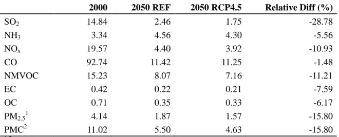
(http://www.airqualitymodeling.org/cmaqwiki/index.php?title=CMAQv5.0_GSPRO_Example, accessed 5 September 2013) (Table A.1). If multiple sources are included in one IPCC sector (e.g., energy and industries in Table A.1), we use the mass ratio from the source that contributes the largest fraction by referring to previous studies (Reff et al., 2009; Xing et al., 2013). Then we calculate the total PM2.5 and PMC in each grid cell by dividing the reported EC and OC by their emission fractions individually, and average these two. By doing this, we increase the total PM2.5 emissions of the RCPs by incorporating the inorganic components of primary PM, such as sulfate and nitrate. We check these results by comparing the total 2000 PM2.5 emissions of 4.14 Tg yr-1 in this study (Table 2.2) with other studies, finding that it is comparable to the total of 4.69 Tg yr-1 in 2001 from the U.S. NEI (http://www.epa.gov/ttnchie1/trends/, accessed 5 October 2013). Our calculated PM2.5 emission is also lower than the estimated 5.53 Tg yr-1 in 2000 by Xing et al. (2013), which used an activity data based approach to develop consistent temporally-resolved emissions from 1999 to 2010.
in 2050 (28.78%). Large spatial variations in emissions reductions are also seen over the U.S., with the largest reductions seen on the east and west urban areas of U.S. for most air pollutants and smaller reductions in the Great Plains (Fig. A.4-A.10).
Biogenic emissions are estimated using the Biogenic Emission Inventory System (BEIS v3.14), which responds to the changing climate for different scenarios. It is configured to run on-line in CMAQ, and calculates the emissions of 35 chemical species including 14 monoterpenes and 1 sesquiterpene. We assume that land use and land cover will stay constant in the future for the purpose of estimating biogenic emissions. The on-line option of lightning is also turned on to calculate the NOx emissions by estimating the number of lightning flashes based on the modeled convective precipitation, which also changes with climate. We prepare the ocean/land mask for the domain to calculate sea salt emissions which can be significant in coastal environments (Kelly et al., 2010). We also use the BEIS on-line calculation for natural soil NOx emissions.
2.2.3 Regional air quality model and dynamical chemical BCs
The latest CMAQ model (https://www.cmascenter.org/cmaq/index.cfm, accessed 15 June 2012) is used to perform the regional air quality simulations with the CB05 chemical mechanism and updated toluene reactions. The model incorporates the newest aerosol module (AE6),
including features of new PM speciation (Reff et al., 2009), oxidative aging of primary organic carbon (Simon and Bhave, 2012), and an updated treatment and tracking of crustal species (e.g., Ca2+, K+, Mg2+) and trace metals (e.g., Fe, Mn) (Fountoukis and Nenes, 2007). Several other enhancements in v5.0 of CMAQ were discussed by Appel et al. (2013) and Nolte et al. (2015), and there are no significant changes for the aerosol module between v5.0 and v5.0.1
configured with 34 vertical layers, with the lowest level being 34 m high, to the highest level at 50 hPa. The horizontal resolution is 36 km by 36 km for the CONUS domain. PM2.5 is calculated from the CMAQ output as the sum of the species EC, OC, secondary organic aerosol (SOA), non-carbon organic matter (NCOM), nitrate (NO3-), sulfate (SO42-), ammonium (NH4+), sodium (Na+), chloride (Cl-), eight crustal and trace metal species, and other unspeciated fine PM (OTHER).
The dynamical BCs for this study are provided by the global MZ4 simulations of
WEST2013. The hourly boundary values from MZ4 are horizontally interpolated from coarser resolution to the regional finer resolution, and also vertically interpolated as MZ4 and CMAQ have different vertical layers. Chemical species are mapped between MZ4 and CMAQ v5.0.1, due to the different chemical mechanisms used by these two models, following the descriptions of Emmons et al. (2010) and ENVIRON (
http://www.camx.com/download/support-software.aspx, accessed 19 September 2013). For the chemical species in CMAQ that do not exist in MZ4, values are set to defaults as suggested by the CMAQ website.
2.2.4 Scenarios
We simulate scenarios in CMAQ comparable to WEST2013, except that we carry out one extra scenario to quantify the co-benefits from domestic versus foreign GHG mitigation (Table 2.1). S_2000 is conducted to evaluate CMAQ model performance and to compare with future scenarios. For this study, we run four scenarios in 2050. The differences between S_RCP45 and S_REF are the total co-benefits on U.S. air quality from global GHG mitigation. The emission benefit from the first mechanism is calculated as the difference between S_Emis and S_REF, and the meteorology benefit is calculated as S_RCP45 minus S_Emis. By comparing S_Dom
with S_Dom, we quantify the co-benefits from domestic and foreign GHG mitigation. In
estimating the co-benefits of domestic reductions, we account for the influences of global climate change as a foreign influence (as most GHG emissions are global), assuming that U.S. air
pollutant emissions have small effects on global or regional climate, such as through aerosol forcing. In each scenario, we fix global methane at concentrations given by the RCPs (Table 2.1), and account for methane changes as a foreign influence, neglecting the fraction of global
methane emissions that are from the U.S. All scenarios are set up as continuous runs, with S_2000 running from September, 2000 to December, 2003, with the first four months in 2000 as spin-up. The future scenarios are run from September, 2049 to December, 2052 with the months in 2049 as spin-up. Results are presented as the average of three years.
2.3 Results
2.3.1 CMAQ model evaluation
The CMAQ model has been broadly used to study regional future air quality (Hogrefe et al., 2004; Tagaris et al., 2007; Nolte et al., 2008; Lam et al., 2011; Gao et al., 2013) and has been evaluated in many applications (Appel et al., 2010, 2011, 2013; Nolte et al., 2015). Here we evaluate the CMAQ v5.0.1 performance by comparing the model outputs from S_2000 with observations in 2000 from the Interagency Monitoring of PROtected Visual Environments (IMPROVE; http://vista.cira.colostate.edu/improve/, accessed 9 May 2014), the Chemical Speciation Network (CSN; previously known as STN,
http://www.epa.gov/ttn/amtic/speciepg.html, accessed 9 May 2014), and the Clean Air Status and Trends Network (CASTNET; http://epa.gov/castnet/javaweb/index.html, accessed 9 May 2014) for total PM2.5 and its components, and the EPA Air Quality System (AQS;
O3. We pair the model outputs with observations in space and time, and calculate four groups of statistics to evaluate model performance: Median Bias (MdnB, µg m-3 for PM2.5 and ppb for O3), Normalized Median Bias (NMdnB, %), Median Error (MdnE, µg m-3 andppb) and Normalized Median Error (NMdnE, %) (Appendix A). Median metrics are used here instead of the mean, as for data with non-normal distributions (i.e., PM species) the median gives a better representation of the central tendency of the data (USEPA 2007). For O3 evaluation, we use both the maximum daily 1-hour (1hr_O3) and Maximum Daily 8-hour Average (MDA8), and also calculate these metrics with a cutoff value of 40 ppb for the observed O3 to evaluate the model’s reliability in predicting ozone values relevant for the NAAQS (USEPA, 2007). Model performance is not expected to be perfect as meteorology does not correspond with actual year 2000 meteorology, and emissions are derived from global datasets rather than specific emissions for the U.S.
For total PM2.5, overall model performance is good and the NMdnE for IMPROVE and CSN are less than 50%, with slight differences in performance (Table 2.3). CMAQ
underestimates PM2.5 in these two networks and also its components in all three networks (Table A.2), except that it overestimates SO42- compared with IMPROVE, and NH3+ with CSN.
2.3.2 Air quality changes in 2050
Here we show the seasonal and spatial patterns of future air quality changes centered in 2050 relative to 2000 from REF and RCP4.5 (Figs. A.11 to A.14). The three-year seasonal averages of PM2.5 over the entire U.S. decrease in 2050 in both S_REF and S_RCP45 compared with S_2000, especially in the Eastern U.S. and California (CA). The seasonal decreases are largest in winter, with U.S. averages in S_REF (S_RCP45) of 4.42 (4.88) µg m-3, and lowest in the summer of 1.55 (2.00) µg m-3, with annual average of 2.76 (3.23) µg m-3. The three-year seasonal averages of O3 decrease significantly in summer in both the east and west coast, with U.S. average of 6.31 (9.50) ppb in S_REF (S_RCP45). O3 increases over the Northeast and West U.S. in winter in both S_REF and S_RCP45, caused by the weakened NOx titration as a result of the large NOx decrease in the two scenarios (Table 2.2), as also reported in other studies (Gao et al., 2013; Fiore et al., 2015). The magnitude of the decreases between S_REF and S_2000 is lower than that between S_RCP45 and S_2000, as the REF scenario did not apply a GHG mitigation policy, and thus has less emission reductions.
changes in 2050 for S_REF relative to 2000 between CMAQ and MZ4 are similar, except that the magnitudes of the changes are smaller than those for S_RCP45 (Fig. A.15).
2.3.3 Total co-benefits for U.S. air quality from global GHG mitigation
Projected three-year average PM2.5 concentrations in 2050 in both scenarios (S_REF and S_RCP45) are higher in the Eastern U.S. and the west coast of CA, and lower in the Western U.S. (Fig. 2.3). The total co-benefits for U.S. air quality (S_RCP45 minus S_REF) show notable decreases of major air pollutants in 2050. The total co-benefits for PM2.5 over the U.S. show a significant spatial gradient over the U.S. domain, greatest in the eastern U.S., especially urban areas, as well as CA, ranging from 0.4 to 1.0 µg m-3, and least in the Rocky Mountains and Northwest with values below 0.4 µg m-3. The total co-benefits for PM2.5 averaged over the U.S. is 0.47 µg m-3, with the largest contribution from organic matter (OM, including primary OC, SOA and NCOM), accounting for the 45% of the total (0.21 µg m-3), followed by sulfate (0.11 µg m-3) and ammonia (0.05 µg m-3) (Fig. A.16). The total co-benefits are highest in fall, with U.S. domain average of 0.55 µg m-3, and lowest in spring (0.41 µg m-3) (Fig. 2.4). Notice that the region with greatest co-benefits shifts from Central areas in winter and spring to the East in summer and fall, with the largest component of OM also shifting from primary OC to SOA (Fig. A.17).
ppb, unlike PM2.5 which is higher over urban regions. The uniformity of the total O3 co-benefits suggests that they are strongly influenced by global O3 reductions.
The total co-benefit for PM2.5 from this study (0.47 µg m-3 over U.S.) is lower than WEST2013 (area-weighted three-year averages of 0.72 µg m-3 over U.S.), especially over the Northwest and Central of U.S. (Fig. A.18). Analyzing the components of PM2.5, we find that this difference is mainly caused by OM, with a U.S. annual average of 0.40 µg m-3 in WEST2013 and 0.21 µg m-3 in this study (Fig. A.19). For other components (EC, SO42-, NO3- as reported in MZ4 of WEST2013), the CMAQ results are slightly lower than WEST2013 but share a similar spatial pattern (Fig. A.20-A.22). We expect that the total co-benefits of PM2.5 in this study might be higher than WEST2013, as we account for inorganic primary PM emissions in SMOKE. A possible explanation may be that different chemical mechanisms and deposition processes are adopted for organic aerosols in MZ4 and CMAQ, which may make a shorter atmospheric lifetime for PM in CMAQ than that in MZ4. The differences of the meteorology (e.g., the precipitation and temperature) between the downscaled WRF and the GFDL could also contribute to this difference. Total co-benefit of O3 from this study (3.55 ppb over U.S.) is comparable to WEST2013 (3.71 ppb) in both the magnitude and spatial distribution (Fig. A.23).
2.3.4 Co-benefits from the two mechanisms
from OM (0.172 µg m-3over the U.S.), followed by sulfate (0.107 µg m-3) and ammonia (0.048 µg m-3). Slowing climate change only accounts for 4% of the U.S. average total PM2.5 decreases (0.02 µg m-3). It also has different signs of effect over the U.S., reducing PM2.5 in the Southern U.S. but increasing in the North.
For O3, the emission benefit is also larger than the climate benefit, accounting for 89% of the total O3 decreases averaged over the U.S. The emission benefit for O3 over the U.S. domain is 3.16 ppb, and much more uniform over the U.S., slightly higher over Northeast and Northwest. Slowing climate change accounts for 0.39 ppb O3 decreases, 11% of the total and mainly in the Great Plains and the East, where temperatures are cooler under RCP4.5 compared with RCP8.5 (Fig. 2.1). The dominance of the emission co-benefit over the climate co-benefit for both PM2.5 and O3 is consistent with WEST2013.
2.3.5 Co-benefits from domestic and foreign GHG mitigation
For O3, foreign countries’ GHG mitigation has a much larger influence on the U.S.,
accounting for 76% (2.69 ppb) of the total O3 decrease, compared with 24% from domestic GHG mitigation (Fig. 2.7). The U.S. experiences greater O3 decreases in the North than the South, which is likely influenced in part by the air quality improvement in Western Canada as a result of slowing deforestation due to the climate policy in RCP4.5 (West et al., 2013). This large influence of foreign reductions for O3 highlights the importance of global methane reductions in RCP4.5 and global emission reductions, particularly in Asia and intercontinental transport.
2.3.6 Regional co-benefits and variability
We then quantify the co-benefits over nine U.S. climate regions defined by the National Oceanic and Atmospheric Administration (Fig. A.24), and their domestic and foreign
components. The Central, Southeast, Northeast and South regions have the largest total
co-benefits for PM2.5 (regional annual means of 0.78, 0.75, 0.62 and 0.62 µg m-3), and the Northwest has the lowest total co-benefits (0.16 µg m-3)(Fig. 2.8). Domestic GHG mitigation has the largest effect over these same regions and lowest effects over Northwest and West North Central, with means of 0.13 µg m-3. Foreign co-benefits are greatest over the South, Southwest, Central and Southeast, and lowest over Northwest (Table A.3). As a fraction of the total co-benefits, the domestic co-benefit is highest in the Northeast, East North Central and Central accounting for more than 80% of the total, while foreign co-benefits are highest over Southwest, South and West North Central, accounting for about 40% of the total.
and Southeast, with regional means of 1.25, 1.16 and 1.14 ppb, and lowest over Northwest (0.4 ppb). In general, foreign mitigation contributes more in the west than the east, most likely influenced by intercontinental transport from Asia. It is highest in the Northwest, West North Central and Northeast, with regional means of 3.75, 3.45 and 3.45 ppb. The fraction of co-benefits from foreign mitigation is larger than 60% in most regions, highest over the Northwest (90%), and lowest over the Southeast (57%).
We also evaluate the variability in co-benefits for the three years simulated (Table A.3). Over the U.S., the coefficient of variation (CV) for the total co-benefits for PM2.5 (7%) is much lower than that of the total co-benefits for O3 (37%), which is controlled by the intercontinental transport and global CH4. The Southeast has the highest CV (29%) for the total co-benefits of PM2.5, while other regions are lower than 15%, lowest in the East North Central and Northeast (3%). Southwest and South have the highest CV (70%, 69%) for the total co-benefits of O3, and lowest in Northwest (21%). For regions with higher variability, longer simulations would be desirable to better quantify the annual average co-benefits.
2.4 Discussion
The co-benefits we present here are specific to the reference (REF) and mitigation (RCP4.5) scenarios we choose, and results would differ for other baseline and mitigation scenarios. The estimated co-benefits also depend on participation of many nations in the mitigation policies, and delaying participation will likely change the co-benefits.
mechanisms between the global and the regional model. The resolution we are using for this study (36km by 36 km) is fine enough for us to analyze the co-benefits at a state level, but insufficient to fully resolve urban areas. Finer resolution simulations (such as 12 km by 12 km) with CMAQ or other CTMs can be carried out to better quantify the co-benefits over urban areas.
For this study, uncertainties and errors may exist under the assumptions and choices we make for each model. For example, the co-benefits of PM2.5 have large contributions from OC and SOA over the Central and East U.S. (Fig. 2.4, Fig. A.16). However, our model evaluations show that CMAQ greatly underestimates the OC concentration compared with surface
observations. We have not included the model evaluation for the SOA due to the limitation of the observation datasets, even though recent studies found that the CMAQ also greatly
underestimated the SOA species (Baek et al., 2015; Hayes et al., 2015; Woody et al., 2015). New gas-phase and aqueous-phase oxidation pathways for SOA formation are found to play
significant roles in producing organic aerosols (Lin et al., 2014; Pye and Pouliot, 2012; Pye et al., 2013), which are missing in the CMAQ version used in this study. The underestimation of the both OC and SOA in the current CMAQ model would greatly reduce the total co-benefits on both air quality and reduced premature mortality estimated from this study. We use BEIS model to estimate the biogenic VOC (BVOC) emissions, but studies have shown that the BVOCs from the Model of Emissions of Gases and Aerosols from Nature (MEGAN) are higher than those from BEIS by a factor 2 (Pouliot, 2008; Pouliot and Pierce, 2009), which highlights the uncertainty in representing these emissions and simulating both PM2.5 and O3 (Hogrefe et al., 2011).
results (Unger, 2014; Heald and Spracklen, 2015). When we process the global anthropogenic emissions with SMOKE, we back-calculate the total PM2.5 and PMC from OC and BC, which introduces inorganic PM emissions and may make our results for co-benefits of PM2.5 higher. By doing this, we account for missing emissions but also increase the total uncertainties in the emission inventory. Spectral nudging is adopted in this study to restrain WRF from drifting from the GCM, which has been shown to be better for some meteorological variables, but spectral nudging better for others (Bowden et al., 2012, 2013; Liu et al., 2012; Otte et al., 2012).
Moreover, only one model is used at each step during downscaling, and ensemble model means can be used to reduce the single model’s variability. Simulations are based on three-year
averages, due to computational limitations, but these three years may reflect meteorological variability and not only climate change. This uncertainty may be greater for the total co-benefits of O3, for which we see greater year-to-year variations than for PM2.5. CMAQ simulations could be performed over more years to reduce the influence of the climate variability. In separating domestic and foreign co-benefits, we assume that global and regional climate will be controlled by foreign GHGs emissions, and not influenced by GHG mitigation in the U.S., which may also introduce errors into our results. We similarly attribute the global methane change as a foreign influence, as U.S. methane emissions are a small fraction of the global.
2.5 Conclusions
Climate polices to control GHG emissions will not only have the benefit of slowing climate change, but can also have co-benefits of improved air quality. Previous co-benefits studies focus mostly on local or regional GHG reductions. As a result, these studies omit air quality benefits outside of the domain considered, and neglect benefits from global GHG
global and regional GHG mitigation on regional air quality over U.S. at fine resolution in 2050, building on the global co-benefits study from West et al. (2013). The co-benefits of global GHG mitigation on U.S. air quality are discussed through two mechanisms: reduced co-emitted air pollutants and slowing climate change and its influence on air quality. We also quantify the co-benefits from domestic GHG mitigation versus foreign countries’ reduction.
We find that there are significant benefits for both PM2.5 and O3 over U.S. by 2050 from the global GHG mitigation in RCP4.5. The total co-benefits for PM2.5 are higher in the east than the west, with an average of 0.47 µg m-3 over U.S. For O3, the total co-benefits are fairly uniform across the U.S. at 2-5 ppb, with U.S. average of 3.55 ppb. The benefits from reductions of co-emitted air pollutants have a greater influence on both PM2.5 (accounting for 96% of total
decreases) and O3 (89% of the total decreases) than the second mechanism via slowing climate change, consistent with West et al. (2013).
2.6 Figures and Tables
Table 2. 1. List of CMAQv5.0.1 simulations in this study. Hourly BCs are from the MOZART-4 (MZ4) simulations of WEST2013. We fix the methane (CH4) background concentrations in CMAQ consistent with the RCP scenarios and WEST2013.
Years Scenario Emissions Meteorology BCs CH4
2000 S_2000 2000 2000 MZ42000 1766 ppbv
2050
S_REF REF RCP8.5 MZ4 REF 2267 ppbv
S_RCP45 RCP4.5 RCP4.5 MZ4 RCP4.5 1833 ppbv
S_Emis RCP4.5 RCP8.5 MZ4 e45m85b 1833 ppbv
S_Dom RCP4.5 for U.S., REF for Can, Mexa
RCP8.5 MZ4 REF 2267 ppbv
a
the part of Canada and Mexico in the domain. b
Table 2. 2. Anthropogenic emissions in the U.S. for major air pollutants in 2000 and 2050 from REF and RCP4.5 (Tg yr-1), and the relative differences (Relative Diff)
between RCP4.5 and REF in 2050 ((RCP4.5 - REF)/REF×100).
2000 2050 REF 2050 RCP4.5 Relative Diff (%)
SO2 14.84 2.46 1.75 -28.78
NH3 3.34 4.56 4.30 -5.56
NOx 19.57 4.40 3.92 -10.93
CO 92.74 11.42 11.25 -1.48
NMVOC 15.23 8.07 7.16 -11.21
EC 0.42 0.22 0.21 -7.59
OC 0.71 0.35 0.33 -6.17
PM2.51 4.14 1.87 1.57 -15.80
PMC2 11.02 5.50 4.63 -15.80
1,2
Table 2. 3. Evaluation of the S_2000 simulation (average of three years modeled) with surface observations in 2000 for PM2.5 (µg m-3) and O3 (ppb).
2000 2050 REF 2050 RCP4.5 Relative Diff (%)
SO2 14.84 2.46 1.75 -28.78
NH3 3.34 4.56 4.30 -5.56
NOx 19.57 4.40 3.92 -10.93
CO 92.74 11.42 11.25 -1.48
NMVOC 15.23 8.07 7.16 -11.21
EC 0.42 0.22 0.21 -7.59
OC 0.71 0.35 0.33 -6.17
PM2.51 4.14 1.87 1.57 -15.80
PMC2 11.02 5.50 4.63 -15.80
1,2
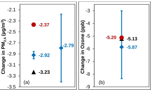
Fig. 2. 2. Comparison of annual U.S. average concentration changes for RCP4.5 in 2050 relative to 2000, for this study (black triangle), MZ4 from WEST2013 (red circle), and the ensemble mean (blue diamond) and multi-model range from ACCMIP (blue lines), for (a) PM2.5, and (b) O3. In panel a, the total PM2.5 reported by the ACCMIP models is shown on the left, and the PM2.5 estimated as a sum of species BC+OA+SOA+SO4+NO3+NH4+0.25*SeaSalt+0.1*Dust following Fiore et al. (2012) and Silva et al. (2013) shown on the right. Values shown are the average of three years for CMAQ and MZ4, and 5 to 10 years for ACCMIP for three models (LMDzORINCA, GFDL-AM3 and GISS-E2-R) that report O3 and two models (GFDL-AM3 and GISS-E2-R) that report PM2.5.
-2.92 -2.79 -2.37 -3.23 -3.5 -3.3 -3.1 -2.9 -2.7 -2.5 -2.3 -2.1 C hange in P M2.5 ( µ g/ m 3) -5.87 -5.13 -5.20 -9 -8 -7 -6 -5 -4 -3 C hange in O z one ( ppb)
Fig. 2. 8. Mean values of domestic (blue) and foreign co-benefits (red) for U.S. average (a) annual PM2.5, and (b) ozone season MDA8 O3. The numbers below each bar are the percentage (%) of the foreign co-benefit.
25% 25% 38% 47% 40% 16%
17% 17%
15% 26% -1 -0.9 -0.8 -0.7 -0.6 -0.5 -0.4 -0.3 -0.2 -0.1 0 PM 2 .5 µg m -3 Domestic Foreign (a)
90% 74% 86%
75% 72%
CHAPTER 3. CO-BENEFITS OF GLOBAL, DOMESTIC, AND SECTORAL
GREENHOUSE GAS MITIGATION ON US AIR POLLUTION AND HUMAN HEALTH IN 2050
(Yuqiang Zhang, Steven J. Smith, J. Jason West. In preparation for submission to
Environmental Research Letter)
3.1 Introduction
Exposure to fine particulate matter (PM2.5) and ozone (O3) are associated with both morbidity (e.g. hospitalizations, emergency department visits, school loss days and asthma-related health effects) and premature mortality (e.g. deaths from cardiovascular and respiratory diseases, lung cancer and so on), as revealed in epidemiological studies (US EPA, 2009, 2013). Several cohort studies have shown evidence of the PM2.5 chronic effects on mortality (Laden et al., 2006; Krewski et al., 2009; Lepeule et al., 2012). One report from Jerrett et al. (2009) demonstrated the chronic effect of O3 on human mortality.