Toward an understanding of the indirect climatic effect of aerosols

(1)

Aerosols

Thesis by

Athanasios Nenes

In Partial Fulfillment of the Requirements

for the Degree of

Doctor of Philosophy

California Institute of Technology

Pasadena, California

2003

(2)

c

° 2003 Athanasios Nenes

(3)

All men by nature desire to know.

Aristotle (Metaphysics).

(4)

Acknowledgements

I never thought that the years spent at Caltech would have such a profound effect on

me. It is not only because of the quality and level of science that takes place here; that is

well known. It is also the extraordinary people that I’ve gotten to know and become friends

with, that have made these years special.

First, I would like to thank John Seinfeld for being a wonderful advisor. He gave me

the opportunity to work in an exciting field, he let me choose my own research path, he

has been very understanding and supportive during times of personal need, and always has

been there to provide guidance and professional support. I couldn’t ask for a better mentor

and truly thank him for helping me realize a dream. I would also like to thank Rick Flagan

for his help over the years, for all the interesting and challenging conversations, and for

constantly reminding me what love for science is all about.

I would like to thank my friend and colleague Timothy Vanreken for all the fun we had

throughout the difficult years of grad school, for not hating me too much when projects

changed direction, and simply for being there when needed the most. Likewise, I would

also like to thank Peter Adams for his friendship and help during all these years. Both

of you guys have been like a “family away from home”. I hope that will never change. I

would also like to thank Serena Chung, for being such a great officemate, musical partner

and friend. I would like to thank all of the other members of the Seinfeld group, and in

particular, Patrick Chuang (who also showed me some excellent restaurants), Don Collins,

Rob Griffin, Bill Conant, Julia Lu, Tracey Rissman, David Katoshevski, and Greg Roberts.

I will always remember their friendship and have enjoyed working with them all.

(5)

has always generously offered help and advice whenever seeked for, and Bob Charlson, for

our many long and interesting discussions.

Many people made sure my life here wasn’t just science. Delores Bing and Allen Gross

provided many opportunities to play music in the Caltech music program and the

Occiden-tal College Orchestra. I was fortunate to play with very Occiden-talented musicians, particularly

Alex Dunn and Todd Murphey. I thank them both for the many moments of beautiful

music. I would also like to thank the St. Anthony’s Greek Orthodox Church for entrusting

me the role of organist during the past three years. Getting up at 8AM (give or take a

few minutes) every Sunday morning wasn’t always easy; nevertheless, it was well worth it.

Getting to know the choir director, Dr. Dimitrios Antsos, was another stroke of luck. His

friendship (and vast knowledge of music) is truly a treasure.

Of course, I cannot neglect to thank the “Latino crowd” for all the legendary parties,

asados, dinners, Semana Latina’s....

From thousands of kilometers away, I am grateful to my parents Theodosi and Maria,

and my brothers Anastasio and Dimitri, for constantly providing love and support for as

long as I can remember.

And finally, I would like to thank Luz. Her love, support and companionship has been

(6)

Abstract

This thesis is motivated by the need to improve our understanding of the aerosol indirect

effect. The activation of aerosol into cloud droplets has been extensively studied, using a

comprehensive numerical cloud droplet activation model. Using this model, the effect of

water vapor mass transfer limitations on the cloud droplet activation process was first

studied; it was found that mass transfer limitations are important for activation under

polluted conditions. The potential effect of (currently unresolved) “chemical effects” on

cloud droplet number (e.g., the presence soluble gases and surface active species) was also

assessed. It was seen that small changes in aerosol and gas-phase composition can have a

strong effect on cloud droplet number, and should be included in future estimates of the

aerosol indirect effect.

A comprehensive aerosol activation parameterization was developed for use in a

first-principle assessment of the aerosol indirect effect. This new parameterization introduces the

concept of “population splitting,” in which the droplets are separated into two populations,

each with its own growth characteristics. The effect of water vapor mass transfer limitations

is explicitly introduced. The parameterization allows for treatment of chemical effects. The

new parameterization shows excellent and robust agreement with a detailed numerical parcel

model.

Previously unidentified mechanisms of aerosol-cloud interactions were also explored.

Aerosol, when it contains black carbon, can absorb light and heat the droplet enough to

affect its activation behavior. This can affect cloud properties in numerous and

counterin-tuitive ways; black carbon heating can dissipate clouds, but may also increase cloud lifetime

(and lead to a climatic cooling) by decreasing the probability of drizzle formation.

Finally, the performance of instruments used for measuring the concentration of cloud

condensation nuclei (CCN) was assessed. Each design exhibits different limitations and

(7)

su-persaturation (< 0.1%). The performance of the instrumentation can be very sensitive

to the operating conditions. Therefore, an depth theoretical understanding of the

in-strumentation is necessary; otherwise, CCN measurements may be subject to considerable

(8)

List of Figures

1.1 Radiative budget of Earth’s climate. Red boxes indicate regions where clouds

are influential [76]. . . 2

1.2 Satellite picture at 3.5 µm wavelength of ship tracks off the West Coast of the

United States [143]. . . 3

1.3 Global, annual-mean radiative forcings (Wm−₂

) due to a number of agents

for the period from pre-industrial (1750) to present (late 1990s). Bar heights

indicate best estimate value; lack of a bar indicates no estimate is available.

The vertical line about the rectangular bar with “X” delimiters indicates an

estimate of the uncertainty range, for the most part guided by the spread in

the published values of the forcing. A vertical line without a rectangular bar

and with “O” delimiters denotes a forcing for which no central estimate can

be given owing to large uncertainties. A “level of scientific understanding”

index is accorded to each forcing, with high, medium, low and very low levels,

respectively. (Adopted from http://www.cmdl.noaa.gov/info/ipcc.html) . . . 4

1.4 Empirical relationship between cloud droplet number and sulfate mass (adopted

from [131]). . . 5

2.1 Illustration of the kinetic limitation mechanisms. . . 12

2.2 Illustration of the three types of droplet ratio profiles seen in the simulations. 16

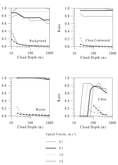
2.3 Droplet ratio as a function of updraft velocity and cloud thickness for the

background, clean continental, marine, and urban distributions of Table 1.

Solid lines represent the droplet ratio α(z), while dashed lines represent the

(14)

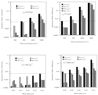
2.4 Maximum difference between thermodynamic and kinetic cloud albedo. The

single mode lognormal distribution aerosol is used with (a) number mode

ra-dius 0.03 µm, (b) number mode radius 0.1 µm, (c) number concentration of

100 cm−₃

, and (d) number concentration of 1000 cm−₃

. . . 29

2.5 Maximum difference between thermodynamic and kinetic cloud albedo. The

aerosol distributions in Table 2.1 are used with (a) given number

concentra-tions, and (d) doubled number concentrations. . . 31

3.1 Typical parcel supersaturation and droplet growth profiles for a rising

adi-abatic cloud parcel. In this calculation, the parcel rises with a velocity of

0.1 m s−₁

. The aerosol in the parcel has a typical marine size distribution

and is composed entirely of (NH4)2SO4. The initial parcel conditions are 98%

relative humidity, 800 mbar pressure, and 283 K temperature. Red curves

cor-respond to particles that form cloud droplets. Blue curves represent particles

with critical supersaturation too high to activate. The green curve corresponds

to a particle that could activate but is not exposed sufficiently long to a

su-persaturation to cause activation. The particle with the smallest dry size that

activates into a cloud droplet has a dry diameter of 0.095µm; its corresponding

K¨ohler curve is shown in the insert. . . 41

3.2 Surface tension decrease with respect to pure water as a function of water

soluble organic carbon (WSOC) concentration (expressed as moles per liter

of carbon) of cloud/fog water samples collected at Tenerife (Canary Islands)

and in the Po Valley (Italy). The observed data are fitted by the

empir-ical Szyszkowski-Langmuir equation (9), σ = K ₋ βTln(1 + αC), where

K = 72.8 kN m−1

, and C is the WSOC concentration (mol C L−1

). The

values of the empirical parameters, β and α, are β = 87 kN m−₁

K−₁

and

α(L mol−1

) is 179.9 for Po Valley 1, 628.1 for Po Valley 2, 302.1 for Tenerife

1, and 888.9 for Tenerife 2. Uncertainty associated with surface tension

mea-surements is less than 0.5%, while WSOC concentration uncertainty does not

(15)

3.3 Ambient saturation ratio in two fog simulations, with gas-phase HNO3 mixing ratios of 0.1 and 30 ppb, the former a “clean” case and the latter corresponding

to polluted conditions. The ambient cooling rate is 1 K h−1

, corresponding

to observations of radiative cooling during fog formation (32). Initial relative

humidity is 98%, and initial aerosol size distributions are log normal, consisting

of two modes, each having two submodes. Particles consist of ammonium

sulfate and insoluble material, as discussed by Kulmala et al. (26). Values are

shown in Table 3.1. . . 46

3.4 Maximum albedo difference with respect to the baseline simulation, for a

con-vective marine cloud, (a) CCN containing 10% by mass insoluble material, (b)

CCN containing 10% by mass of water-soluble organic carbon (no surface

ten-sion effects), (c) CCN containing 10% by mass of water-soluble organic carbon

(with surface tension effects), (d) completely soluble inorganic aerosol, initial

gas-phase HNO3 at 5 ppb, and (e) completely soluble inorganic aerosol, with concentrations doubled. The organic fraction is assumed to be composed of

18% (by mass) levoglucosan (C6H10O5, molar mass = 0.162 kg mol−1, density = 1600 kg m−₃

, van’t Hoff factor = 1), 41% (by mass) succinic acid (C6O4H6,

molar mass = 0.118 kg mol−₁

, density = 1572 kg m−₃

, van’t Hoff factor =

3), and 41% (by mass) fulvic acid [Suwanee River certified FA standards, US

Geological Survey, Report 87-557, 1989] (C33H32O19, molar mass = 0.732 kg mol−₁

, density = 1500 kg m−₃

, van’t Hoff factor = 5). . . 48

3.5 Maximum albedo difference with respect to the baseline simulation, for a

con-vective urban cloud, (a) CCN containing 50% by mass insoluble material, (b)

CCN containing 50% by mass of water-soluble organic carbon (no surface

ten-sion effects), (c) CCN containing 50% by mass of water-soluble organic carbon

(with surface tension effects), (d) completely soluble inorganic aerosol, initial

gas-phase HNO3 at 5 ppb, and (e) completely soluble inorganic aerosol, with

concentrations doubled. The organic fraction is assumed to be the same as for

(16)

3.6 Isopleth contours of maximum albedo difference with respect to the logarithm

of solubility (moles L−₁

) and organic mass fraction of aerosol. Surface

ten-sion effect is as described in the caption of Figure 3.2. The organic fraction

is assumed to be the same as for Figure 3.4. Marine (a) and urban (b)

con-vective clouds with an updraft velocity equal to 1 m s−₁

are assumed in these

calculations. . . 53

4.1 Droplet number concentration normalized to the baselineNd, as a function of

updraft velocity, for marine aerosol size distributions. . . 63

4.2 Same as Figure 4.1, but for the urban size distribution. . . 64

4.3 Isopleth contours of cloud droplet number concentration change (%) relative

to the baseline simulation, with respect to the logarithm of solubility (moles

L−₁

) and organic mass fraction of aerosol. Theσeffects are as described in the

text. Marine conditions and an updraft velocity equal to 1 m s−₁

are assumed

in these calculations. . . 64

5.1 Summary of cumulative CCN spectra measured for wet, transition and dry

seasons in the Amazon Basin. The error bars indicate one sigma variation

in the CCN spectra normalized to its highest supersaturation, except for the

error bars at the highest supersaturation of each spectrum. ** These error

bars represent one sigma variation in the CCN number concentration for the

selected sample period. . . 75

5.2 Modelled and measured CCN spectra for the wet and dry season. The

simu-lations (WA, WB, etc.) are defined in Table 5.1. . . 78

5.3 Cloud parcel maximum supersaturation as a function of increasing aerosol

con-centrations using the wet-season forest site CCN number distribution (WA).

Each curve represents a different updraft velocity. . . 80

5.4 Fraction of aerosol that serves as CCN, f_CCN/CN, for the measured CCN

spectra in the Amazon Basin. The error bars in this and the following figures

represent one-sigma variations for a particular season using the simulations

(17)

5.5 Ratio of cloud droplet concentration between the measured CCN spectra in the

Amazon Basin and the wet season. The wet-season forest site CCN spectrum

was used as a reference. . . 82

5.6 Ratio of effective cloud radius between the measured CCN spectra in the

Amazon Basin and the wet season. The wet-season forest site CCN spectrum

was used as a reference. . . 83

5.7 Predicted effective cloud radius as a function of increasing aerosol

concentra-tions for a variety of cloud depths. The wet-season forest site CCN spectrum

was used with an updraft velocity of 0.3 m s−₁

. The cloud depth is indicated

on each line. . . 84

5.8 Predicted maximum albedo differences among measured CCN spectra in the

Amazon Basin for different updraft velocities. The aerosol distributions in

Table 1 are used and the wet-season forest case is used as a reference. The

dashed lines represents a climatically significant radiative forcing of 1 W m−₂

or a change in cloud albedo of 0.005. . . 86

5.9 Maximum differences between thermodynamically and kinetically predicted

cloud albedo for different updraft velocities. The aerosol distributions in Table

5.1 are used. The dashed lines represent a climatically significant radiative

forcing of 1 W m−₂

or a change in cloud albedo of 0.005. . . 87

5.10 Effective radius for each distribution normalized to the mean. Wet- and

dry-season profiles from Table 5.1 are shown for an updraft velocity of 1.0 m s−₁

.

The shaded area indicates the region of reff within 5% of the mean. The

simulations (WA, WB, etc.) are defined in Table 5.1. . . 89

6.1 Direct and indirect radiative effects of aerosol, divided into those effects

un-related to aerosol absorption (a)-(d), and those related to aerosol absorption

(18)

6.3 Actinic flux under varying conditions of cloudiness and surface albedo. (a)

Vertical profile of actinic flux calculated for 3 cases: no cloud, cloud with

optical thickness τc = 5, and cloud with τc = 20. Each case considers a solar

zenith angle of 60o_{, ocean surface reflection (albedo} _∼_{0.07 for no cloud case),}

and clouds are horizontally homogeneous. (b)Actinic flux for cloud base and cloud top as a function of cloud optical depths ranging from 0 (no cloud) to

20. Three cases of surface albedo are considered: ocean reflection (explicitly

accounting for both Fresnel and bulk reflection), (b) grassland (isotropic albedo

of 0.26), and (c) snow/ice (isotropic albedo of 0.6). . . 97

6.4 Heating parameter, γa, for dry particles (contour lines) as a function of dry

particle diameter,dp, and spectrally averaged absorption efficiency,Qabs. The

heavy solid and dashed lines represent the relationship between Qabs and dp

for dry aerosols composed of 50% BC by mass and 10% BC, respectively. . . 101

6.5 Effect of droplet heating on the K¨ohler curves of particles of 0.5 µm and 1.0

µm dry diameter. Heating parameters of 0.1 and 0.2 are chosen for the two

droplet sizes, respectively. The solid curve represents the no-heating case, the

dashed curve represents the heating case. Particles are assumed to have the

hygroscopic properties of sulfate. . . 102

6.6 Effect of BC on (a) critical supersaturation, and (b) critical diameter. Four cases are considered: (6.1) 10% BC by mass and no heating; (6.2) 10% BC

and heating by a 1000 Wm−₂

actinic flux; (6.3) and (6.4) same as (6.1) and

(6.2) but for 50% BC by mass. The difference between the no heating cases

(6.1) and (6.3) is caused by the reduced sulfate mass in the 50% BC case

compared to the 10% BC case. The heating effect is apparent as a divergence

between the heating and no heating cases towards large particle sizes. The

perturbation in droplet temperature at critical diameter is shown as the thick,

gray lines in (a). The legend in (b) applies to both (a) and (b). . . 104

6.7 Illustration of the impact of actinic flux on critical supersaturation for(a)50% BC by mass, and (b) 10% BC by mass. The effect of increasing actinic flux is to increase the lowest possible critical supersaturation,slow, for particles of

a given composition and to decrease the dry particle diameter, dlow, at which

(19)

6.8 Change in critical supersaturation computed for dry particles as a function of

particle diameter and absorption efficiency, Qabs. Contours delineate values

of ∆sc. The solid and dashed lines represent the relationship between Qabs

and dp for dry aerosols composed of 100% BC and 10% BC, respectively.

The calculation of ∆sc includes the enhancement of heating caused by the

encapsulation of the soot core in the droplet. . . 106

6.9 (a)-(c) CCN spectrum calculated from size distributions assuming each par-ticle is either pure sulfate, 10% BC by dry mass, or 50% BC. Cases (a)-(b) are

calculated from [160] size distributions, case (c) from INDOEX. Effects of BC

seen in (a)-(c) are partially due to the solute effect (see Figure 6.6.) (d)-(f )

BC heating effect on CCN spectrum. The percent perturbation in CCN

spec-trum between nighttime (no heating) and daytime (heating) corresponding to

(a)-(c), respectively, are shown as a function of supersaturation for both the

10% BC and 50% BC cases. . . 109

7.1 Illustration of the BC heating scenarios considered in this study. . . 121

7.2 Parcel liquid water content (a) and supersaturation (b) profiles for four

differ-ent radiative heating scenarios. Updraft velocity is 0.25 m s−₁

and BC content

is 50%. . . 123

7.3 Parcel droplet activation ratio for the simulations of Figure 7.2. . . 124

7.4 Liquid water content between heating scenarios as a function of cloud depth.

The BC mass fraction is (a) 0.1, and (b) 0.2. The updraft velocity is assumed

to be 0.1 m s−1

. . . 125

7.5 Albedo difference between the curves of Figure 7.4, as a function of cloud

depth. . . 127

7.6 Vertical profiles of average vertical velocity (updrafts and downdrafts), average

and maximum updraft velocity for the stratocumulus cloud trajectories used

(20)

7.7 Growth of GCCN throughout a cloud column that experiences an updraft of

0.25 m s−₁

(the “NoHeat” scenario of the previous section is used to generate

the supersaturation profile). The composition of these particles is assumed

to be 10% (NH4)2SO4, 0-20% BC (the rest is dust). Curves are shown for particles with dry diameter of 5 and 10 µm. The dashed line represents the

threshold size above which the collection efficiency of the droplets is assumed

to become large. . . 130

7.8 Same as Figure 7.7, but for an updraft velocity of 0.5 m s−₁

. . . 131

7.9 Normalized droplet sizes of the heated GCCN with respect to their unheated

size, for the curves in Figure 7.7 . . . 131

7.10 Average size of GCCN as predicted by TEM for (a) pristine cloud conditions

and (b) polluted cloud conditions. The dry diameter of the GCCN is assumed

to be 5µm. The black dashed line indicates cloud base, while the grey dashed

line indicates the size beyond which the GCCN is assumed to effectively initiate

drizzle formation. . . 134

7.11 Same as Figure 7.10, but for a GCCN dry diameter of 10 µm. . . 136

8.1 Illustration of the sectional representation of (a) aerosol number distribution,

nd(Dp), and (b) supersaturation distribution,ns(Dp). . . 144

8.2 Illustration of the two sub-populations used in developing the parameterization.152

8.3 spart/smaxas a function ofsmax. Each curve corresponds to a constant updraft

velocity. . . 155

8.4 spart/smax as a function of updraft velocity. Each curve corresponds to one of

the aerosol types in Table 8.2. smax is computed using the numerical parcel

model of [117]. . . 156

8.5 Parameterization algorithm. . . 158

8.6 Fraction of aerosol that become droplets, as predicted by the new

parameter-ization and the cloud parcel model. . . 162

8.7 Droplet number concentration, as predicted by the new parameterization and

the cloud parcel model. . . 163

8.8 Droplet number concentration, as predicted by the new parameterization and

(21)

8.9 Maximum parcel supersaturation, as predicted by the new parameterization

and the cloud parcel model. . . 164

8.10 Activated droplet ratio, as a function of updraft velocity. Both the cloud

parcel model and parameterization results (with and without the effect of

the organic from changes in surface tension) are shown. The parcel model

simulations include surface tension effects from the dissolved organic. Marine

aerosol composed of 80% (NH4)2SO4 and 20% organic surfactant is used. The organic surfactant behavior is described in the text. . . 166

8.11 Fraction of aerosol that become droplets, as predicted by the [1]

parameteri-zation and the cloud parcel model. . . 168

8.12 Droplet number concentration, as predicted by the [1] parameterization and

the cloud parcel model. . . 168

9.1 The static diffusion cloud chamber (SDCC). . . 174

9.2 Maximum supersaturation (%) in the SDCC as a function of hot and cold plate

temperatures. A linear temperature profile is assumed. Water vapor pressure

is calculated from a correlation given by [143]. . . 175

9.3 The Fukuta continuous flow spectrometer (FCNS). . . 178

9.4 Typical temperature and supersaturation (%) profiles for the FCNS along a

flow section, for developed inlet conditions. . . 178

9.5 The Hudson continuous flow spectrometer (HCNS). . . 179

9.6 Typical supersaturation (%) profiles for the HCNS along a flow section, for

var-ious maximum temperature differences, ∆Tmax (the ∆T at the last segment).

The temperature difference between each segment is assumed to increase with

a constant step (“linear ramp”) on both cold and warm sides. The profiles are

computed using the HCNS numerical model in this paper. . . 180

9.7 The Caltech continuous flow spectrometer (CCNS). . . 181

9.8 Indicative supersaturation (%) profiles for the CCNS along a flow section, for

various maximum temperature differences. The volumetric flow rate is 0.7 l

min−₁

. The profiles are computed using the CCNS numerical model of this

(22)

9.9 The geometries used in the simple models developed for determining the

un-certainty in the temperature boundary conditions for a) the SDCC, b) the

CCNS, and c) the HCNS. . . 191

9.10 Tw−_T_f

Th−Tc contours for the CCNS as a function of paper and water film thickness.

The thickness of the metal wall is assumed to be 1 cm. . . 195

9.11 T

h f−Tfc

Th

w−Twc contours for the HCNS as a function of flow rate and water film

thick-ness. The thickness of the metal wall is assumed to be 1 cm, and no filter

paper is used. . . 198

9.12 Simulated effective radius in the SDCC view window as a function of time for

various initial particles sizes (dry diameter, µm). The temperature difference

between the two plates is assumed to be (a) 2 K (Smax= 0.15%) and (b)7 K (Smax= 1.81%). . . 204 9.13 Simulated particle concentration in the SDCC view window as a function of

time for various initial particles sizes (dry diameter, µm). The temperature

difference between the two plates is assumed to be (a) 2 K (Smax = 0.15%) and (b) 7 K (Smax= 1.81%). . . 205 9.14 Simulated particle size resolution in the SDCC view window as a function of

time for various initial particles sizes (dry diameter, µm). The temperature

difference between the two plates is assumed to be (a) 2 K (Smax = 0.15%) and (b) 7 K (Smax= 1.81%). . . 206 9.15 Supersaturation (%) profiles for different streamlines along the centerline of

the FCNS. . . 208

9.16 Simulated growth curves for various centerline streamlines of the FCNS. The

temperature difference between the tips is 5 K, and the volumetric flow rate

is 20 l min−₁

. . . 208

9.17 Experimental and simulated calibration curves for the CCNS. The different

simulation cases correspond to different values of effective wall temperature

and accommodation coefficients, the values of which are given in Table 9.5. 210

9.18 Predicted resolution ratio RSc

R_Dp for the CCNS, for different values of

˙

Vsheath

˙

Vaerosol.

The Case 3 (Table 9.5) values of effective wall temperature and accommodation

(23)

9.19 Relative critical supersaturation uncertainty as a function of critical

super-saturation, for the CCNS. The uncertainty was predicted using the curves of

Figure 9.18, and the variability of the outlet droplet diameter (calculated by

the model results). . . 214

9.20 Simulated calibration curves for the HCNS, for different temperature profiles,

and a volumetric flow rate of (a) 6 l min−₁

, and (b) 20 l min−₁

. . . 216

9.21 Experimental and simulated calibration curves for the HCNS. Non-dimensionalized

droplet diameter is plotted as a function of critical supersaturation. V is the

total volumetric flow rate, and DT is the maximum temperature difference

between the plates. V˙sheath

˙

Vaerosol = 10 in the simulations. . . 217

9.22 Predicted resolution ratio RSc

RDp for the HCNS, for different temperature profiles,

and a volumetric flow rate of (a) 6 l min−₁

, and (b) 20 l min−₁

. V˙sheath

˙

Vaerosol = 10

in these simulations. . . 219

9.23 Relative critical supersaturation uncertainty as a function of critical

super-saturation, for the HCNS. The uncertainty was predicted using the curves of

Figure 9.22, and the variability of the outlet droplet diameter (calculated by

the model results). Subplot (a) refers to a volumetric flow rate of 6 l min−₁

,

and (b) to 20 l min−₁

. V˙sheath

˙

(24)

List of Tables

2.1 Aerosol distribution parameters (rg,i inµm, Ni in cm−₃

) [160] . . . 22

2.2 Characteristics of α(z) andφ(z) profiles for single lognormal aerosol

distribu-tion runs. αmax is the maximum value of α(z), encountered at zαmax above

cloud base. . . 23

3.1 Initial aerosol size distributions and chemical composition used for the

simu-lations in Figure 3.3 . . . 55

5.1 Size distribution parameters for CCN spectra . . . 76

5.2 Properties of important components used in K¨ohler theory to estimate CCN

activity. . . 77

5.3 Simulated maximum supersaturations as a function of updraft velocity for

different periods in the Amazon Basin. . . 81

5.4 Simulated asymptotic alpha ratios (Nkn/Nth) as a function of updraft velocity

attained in the cloud parcel model for different periods in the Amazon Basin. 83

6.1 Sensitivity of K¨ohler curve to elevated droplet temperature. (When required,

a 10 µm droplet diameter is assumed.) . . . 99

7.1 Aerosol distribution parameters (geometric radiusrg,i inµm, number

concen-tration Ni in cm−3) [160] . . . 120

7.2 Effective radius (at 140 m cloud depth) and maximum supersaturation (%)

for the parcel simulations in Figures 7.4 and 7.5 . . . 124

8.1 Characteristics of single log-normal aerosol distribution runs. Pressure is 800

mbar, and temperature is 283 K. . . 160

8.2 Aerosol distribution parameters (Dg,i inµm, Ni in cm−₃

(25)

8.3 Characteristics of multiple log-normal aerosol distribution simulations. The

range in updraft velocity examined is 0.1 - 3.0 m s−₁

. Pressure is 900 mbar,

and temperature is 273 K. . . 160

8.4 Statistics of the ratio of Nd calculated from new parameterization to Nd

cal-culated from parcel model. . . 165

9.1 Transfer coefficients and source terms for the gas-phase equations. . . 185

9.2 Operating conditions and parameters for the SDCC [Roberts, G., Internal

communication, California Institute of Technology, 1999] . . . 199

9.3 Operating conditions and parameters for the FCNS [46]. . . 200

9.4 Operating conditions and parameters for the HCNS [Hudson et al., 1981;

Hud-son, 1989; Hudson, J. G., Personal communication, 2000]. . . 200

9.5 Operating conditions and parameters for the CCNS [24]. . . 201

9.6 Summary of SDCC simulations. . . 213

9.7 Predicted outlet droplet diameter variability and resulting critical

supersatu-ration uncertainty for the CCNS. . . 214

9.8 Predicted outlet droplet diameter variability and resulting critical

supersatu-ration uncertainty for the HCNS. V˙sheath

˙

(26)

Chapter 1

Preface

1.1

Introduction

It is well established that suspended particulate matter, or aerosols, can have an

impor-tant effect on the planetary radiative balance (Figure 1.1) and thus affect climate. These

climatic effects are roughly classified into two categories. First is the “direct effect”, which

refers to the direct interaction of the aerosol particles with radiation (through scattering and

absorption). Second is the so-called indirect effect, which is the change in cloud properties

that result from changes in the aerosol, which serve as cloud condensation nuclei (CCN).

It is currently believed that the indirect effect tends to cool the planet through two

mechanisms that act primarily upon liquid water boundary layer clouds. The “first” (or

“Twomey,” [156]) indirect effect is an increase in cloud droplet concentration that is a result

of increased cloud condensation nuclei concentrations from anthropogenic emissions. The

resulting clouds are believed to be more reflective, thus cool the planet. The “second”

(or “Albrect,” [10]) effect results from the increased lifetime (because the droplets that

form tend to be smaller in size and thus decrease the probability of precipitation); this

effect would increase the fractional planetary coverage, and also lead to a cooling effect.

These are not the only aerosol-cloud interactions that can affect climate, nor do all such

mechanisms cool the planet. For example, the so-called semi-direct effect, in which heating

released by the short-wave absorbing aerosol (primarily black carbon) tends to impede cloud

formation [61]; this leads to decreases in global cloud coverage, and planetary warming.

Evidence of the indirect effect can be found in many aspects of the climate system.

(27)

J.T. Houghton: “The science of climate change”

(28)

Figure 1.2: Satellite picture at 3.5 µm wavelength of ship tracks off the West Coast of the United States [143].

• CCN concentrations are greater in continental air masses (exceeding 1000 cm−₃

) than

in the marine atmosphere (which rarely exceed 100 cm−3

). At the same time,

conti-nental clouds tend to exhibit greater cloud droplet number concentrations than marine

clouds do. [127].

• Cloud droplet number concentrations tend to increase with increasing aerosol loading. This has been confirmed from modelling studies (e.g., [57, 117]) and from observations

[128, 23].

• The existence of “ship tracks,” linear features of high cloud reflectivity embedded within marine stratus clouds, are caused by aerosols emitted from ship exhausts

(Fig-ure 1.2).

1.2

Current estimates of indirect forcing

Figure 1.3 displays a quantitative comparison of each climatic forcing (including those

from greenhouse gases and aerosol), [76]. Each climatic forcing is expressed as the global

(29)

Figure 1.3: Global, annual-mean radiative forcings (Wm−2

(30)

Figure 1.4: Empirical relationship between cloud droplet number and sulfate mass (adopted from [131]).

imply that the tropospheric aerosol might have a net global cooling effect of the order of the

combined warming effect caused by greenhouse gases, which is estimated to be +2.5(_±10%) W m−₂

. To date, the best estimate of the direct climatic forcing of sulfate aerosols lies in

the range between -0.4 W m−₂

, to within a factor of 2. The indirect forcing effect is believed

to be negative in sign, but the present state of knowledge precludes even an estimate of the

magnitude. The value indicated on the plot refers to the first indirect effect, while estimates

of the second indirect effect are too uncertain even to be assigned a value by the IPCC [76].

To fully understand the indirect climate effect of aerosols, it is necessary to be able to

relate changes in atmospheric aerosol properties to changes in cloud radiative properties.

Key aerosol properties include particle size, number and composition; key cloud properties

are droplet size, number, and cloud liquid water content. Most of the global aerosol models

found in the literature explicitly resolve only aerosol mass from first principles, and cannot

provide information for an explicit treatment of aerosol-cloud interactions. Because of this,

empirical relations (such as that shown in Figure 1.4) have been used to relate aerosol

number (or mass) with and droplet concentration. The first comprehensive study using

(31)

predict cloud droplet number concentrations. The empirical approach, although a quick

way to provide a rough estimate of the magnitude of the indirect effect and uncertainties

[101, 83]; it is far from providing an estimate with high enough level of confidence. The

empirical relationship itself is subject to high uncertainty, at least an order of magnitude;

this is a result of the highly complex numerous processes of aerosol-cloud interactions which

cannot be resolved through a simple correlation with one aerosol property. This is shown by

the [83] study, where several different empirical relationships yielded estimates of the global

annual average indirect forcing between -0.40 W m−₂

and -1.78 W m−₂

. Furthermore, the

chemical composition and concentration of the aerosol, together with the underlying cloud

dynamics, vary strongly with time and location, so that simulations using first principles

seems to be the only viable route towards more confident estimates of the indirect effect.

Physically based approaches to address the aerosol indirect effect have also started to

appear. For example, [21, 22] parameterized the sulfate production to preexisting particles

by condensation of gas-phase sulfuric acid and aqueous oxidation of sulfur dioxide, and used

that for their indirect forcing estimates. [101] and [58] have developed prognostic schemes

of global cloud droplet number and used those to assess sulfate indirect effects. [53, 54]

further introduced a modal aerosol microphysical algorithm to predict CCN concentrations

and assess indirect effects. [140] introduced a physically based methodology for assessing

the first and second indirect effects. All of these studies provide important contributions,

but clearly a substantial amount of work needs to be done, before the confidence level in

these global simulations is improved.

1.3

The challenges of indirect forcing

Understanding the indirect climate effect of aerosols requires establishing a link between

changes in atmospheric aerosol properties to changes in cloud radiative properties. This is

indeed a monumental task. Some of the major issues that involve aerosol-cloud interactions

and their incorporation into GCMs are

• The aerosol mass - aerosol number relationship. Most GCMs handle aerosol on a mass basis, which is sufficient for direct forcing calculations, but cannot be used

for indirect forcing. Aerosol number, size, and composition are the parameters that

(32)

size-resolved aerosol global simulation using a sectional approach. Such algorithms

have started to appear (e.g., [159, 8]). The former study utilizes an algorithm that

con-serves mass, but not number; only [8] uses an algorithm that accurately and efficiently

conserves aerosol number and mass concentrations, a prerequisite for reliable indirect

forcing calculations. Further developments to include size resolved simulations of sea

salt, mineral dust and carbonaceous aerosol would provide the information needed for

an in-depth analysis of the contribution of each species to the indirect effect.

• The treatment of cloud formation in global models. This is probably the largest source of uncertainty surrounding indirect forcing of aerosols. Explicitly resolving

cloud formation in global models is a task that far exceeds anything computationally

feasible, as it covers a wide range of length scales: from hundreds of kilometers (which

are relevant for large scale systems) down to meters (which are relevant for individual

updrafts). The size of a typical global model grid cell is on the order of a hundred

kilometers, and can only resolve the largest of cloud systems. Cloud-resolving large

eddy simulations (LES) can possibly address these small length scales, but global

models are far from being able to achieve this. As a consequence, global models

heavily rely on parameterizations to account for all such sub-grid processes, such as

cloud formation and aerosol-cloud interactions. Current parameterizations are very

simplistic, and unable to capture the complexities of aerosol-cloud interactions. This

is a particularly important issue in the aerosol indirect effect, as all its mechanisms

act on subgrid scales.

• The link between aerosol and cloud droplet formation. This relationship has to consider a multitude of parameters that can affect the formation of cloud droplets,

such as varying aerosol composition, and the behavior of complex (and poorly

under-stood) carbonaceous aerosol. Furthermore, the treatment should allow for generalized

representations of aerosol size and composition, and not rely on prescribed size

dis-tributions (e.g., lognormal). Essential is the ability to account for externally mixed

aerosol; CCN that result from mixing of heterogeneous aerosol populations occurs

frequently, and affects clouds that are most susceptible to changes in aerosol.

The challenges, however, are not limited to the theory and modelling of

(33)

to provide model input and also used for assessment of model performance. For example,

the measurement of CCN concentrations is in itself a challenge; a theoretical understanding

of the different measurement methodologies, in both their strengths and limitations, is

essential for evaluating instrumental uncertainties.

1.4

Organization of Thesis

The motivation of this thesis is to improve our understanding of the complex and

nu-merous mechanisms of aerosol-cloud-climate interactions, and the instrumentation used in

CCN measurements. In Chapter 2, we study the dynamics of aerosol activation into cloud

droplets, and study under which conditions mass transfer limitations on the growth of cloud

condensation nuclei (CCN) may have a significant impact on the number of droplets that can

form in a cloud. In Chapters 3 and 4, the sensitivity of cloud droplet number concentration

to CCN chemical effects (such as dissolution of soluble gases and slightly soluble substances,

surface tension depression by organic substances and accommodation coefficient changes) is

assessed by using a cloud parcel model. Chapter 5 assesses the impact of biomass-burning

aerosol on cloud properties in the Amazon Basin and identifies the physical and chemical

properties of the aerosol that influence droplet growth. Chapters 6 and 7 study previously

unidentified cloud microphysical effects of black carbon inclusions in cloud droplets.

Chap-ter 8 develops a novel parameChap-terization of cloud droplet activation intended for use in a

global model. Chapter 9 theoretically analyzes the behavior and performance of four cloud

condensation nucleus (CCN) instruments. Finally, Chapter 10 presents a summary and

(34)

Chapter 2

Kinetic limitations on cloud

droplet formation and impact on

cloud albedo

Note: This chapter appeared as reference [117].

2.1

Abstract

Under certain conditions mass transfer limitations on the growth of cloud condensation

nuclei (CCN) may have a significant impact on the number of droplets that can form in a

cloud. The assumption that particles remain in equilibrium until activated may therefore

not always be appropriate for aerosol populations existing in the atmosphere. This work

identifies three mechanisms that lead to kinetic limitations, the effect of which on activated

cloud droplet number and cloud albedo is assessed using a one-dimensional cloud parcel

model with detailed microphysics for a variety of aerosol size distributions and updraft

ve-locities. In assessing the effect of kinetic limitations, we have assumed as cloud droplets

not only those that are strictly activated (as dictated by classical K¨ohler theory), but also

unactivated drops large enough to have an impact on cloud optical properties. Aerosol

num-ber concentration is found to be the key parameter that controls the significance of kinetic

effects. Simulations indicate that the equilibrium assumption leads to an overprediction of

droplet number by less than 10% for marine aerosol; this overprediction can exceed 40%

for urban type aerosol. Overall, the effect of kinetic limitations on cloud albedo can be

considered important when equilibrium activation theory consistently overpredicts droplet

(35)

limitations is less than 0.005 for cases such as marine aerosol; however albedo differences

can exceed 0.1 under more polluted conditions. Kinetic limitations are thus not expected

to be climatically significant on a global scale, but can regionally have a large impact on

cloud albedo.

2.2

Introduction

Much of the uncertainty associated with quantifying the indirect climatic effect of

aerosols originates in the complex relationship between aerosols and cloud droplets.

Ap-proximate analytical expressions that predict those aerosol particles that activate to form

cloud droplets have been proposed for implementation in general circulation models (GCMs)

[56, 99, 3]. These parameterizations generally rely on the assumption that particles are at

equilibrium with the ambient (supersaturated) water vapor concentration until activated

as cloud condensation nuclei (CCN). The number of droplets formed in a cloud can

there-fore be estimated from the number of CCN active at the maximum supersaturation in the

cloud updraft. The problem of droplet nucleation parameterization is then reduced to the

problem of determining the maximum supersaturation in the cloud parcel.

The assumption that all particles respond instantaneously to any changes in

supersat-uration leads to a problem: the amount of water absorbed by the largest aerosol particles

when they activate can be larger than the amount of water vapor available in the cloud

parcel. This problem, known for a long time, is not serious when predicting the number

of droplets, because although not activated, these particles have an equilibrium saturation

ratio very close to unity, as activated particles do. As a consequence, their growth can be

parameterized as if they were activated. In addition, the number of large particles that give

rise to this problem are usually negligible compared to the concentration of smaller particles

of the distribution, so the errors in cloud droplet number overall are expected to be small.

The assumption of equilibrium, however, can lead to a discrepancy in droplet number

as a result of mass transfer limitations. [22] have shown that under certain circumstances

growth kinetics may retard the growth of CCN sufficiently to limit the number of activated

droplets formed. By comparing the timescale for particle growth at equilibrium with that

for actual condensational growth, [22] conclude that particles with critical supersaturation

(36)

do not activate. This suggests that equilibrium models that diagnose droplet formation

from maximum supersaturation may systematically overestimate the number of activated

droplets formed. Such a systematic bias could have implications for estimates of indirect

aerosol radiative forcing of climate. It is difficult, however, to draw firm conclusions simply

from a comparison of timescales because growth kinetics depend on the full time history

of supersaturation and particle growth. Furthermore, the timescales controlling the growth

of the droplets change drastically as the populations grow. A more conclusive method of

evaluating the importance of growth kinetics is obtained by explicitly simulating the

ki-netic growth process and then comparing the simulated number of droplets formed with

that predicted by equilibrium theory for the same CCN concentration and maximum

su-persaturation.

Furthermore, it is incorrect to consider cloud drops as only those that are strictly

acti-vated (as defined by K¨ohler theory); the presence of large unactiacti-vated droplets cannot be

neglected. This issue becomes even more important when slightly soluble substances are

present in the aerosol [93]. The condensational growth of an aerosol population prescribes

that particles with very large dry diameters, although not activated, lead to roughly the

same size of activated droplets and thus belong to the cloud droplet population. With this

in mind, one can define as CCN all particles that produce droplets that are larger than the

smallest particle that is strictly activated. This cloud droplet definition differs slightly from

that given by [123]; we do not consider as droplets all the particles that exceed their critical

diameter or have a critical supersaturation lower than ambient supersaturation, but only

those comparable in size to those that are strictly activated.

Based on the previous discussion, the inertial mechanism of [22] is believed not to

contribute to any bias in the predicted droplet number when the equilibrium assumption is

invoked. However, there are other kinetic limitation mechanisms that produce particles that

are much smaller than activated drops; in this sense, these mechanisms act to decrease the

number of cloud droplets from that predicted strictly on the basis of equilibrium activation.

This study will focus mainly on these mechanisms.

In the sections that follow, the mechanisms that lead to kinetic limitations in cloud

droplet formation are presented. The models used for evaluating kinetic effects are then

described, together with the relevant criteria used for assessing the potential climatic

(37)

Figure 2.1: Illustration of the kinetic limitation mechanisms.

and aerosol types, from which conclusions can be derived regarding the effect of kinetic

limitations on cloud droplet number concentration and albedo.

2.3

Kinetic limitation mechanisms

There are three kinetic limitation processes that can inhibit the formation of cloud

droplets. These mechanisms will be explained with the help of Figure 2.1, which illustrates

typical cloud parcel and droplet equilibrium supersaturation profiles (S and Seq,

respec-tively) as a function of cloud depth, as predicted by adiabatic parcel theory. Each aerosol

equilibrium curve corresponds to particles containing a different amount of solute. The

equilibrium curves vary with respect to cloud depth as a consequence of droplets changing

size as they traverse through the cloud column. According to equilibrium activation theory,

any particle with a critical supersaturation, Sc, less than the maximum supersaturation,

Smax, encountered in the parcel will activate. However, the time which particles are exposed to a supersaturation level is a crucial parameter; that time must be sufficiently long to

(38)

when the wet diameter exceeds its critical value. Furthermore, to ensure constant growth

of the droplet, the ambient supersaturation should be high enough for activated droplets to

continuously grow throughout the duration of cloud formation.

The yellow curve of Figure 2.1 represents an aerosol particle that activates and remains so

throughout the entire time of cloud formation. The critical supersaturation of the particle,

Sc3, is less thanSmax; the time needed for activation is also less than the time during which

S _≥Sc3. When this particle activates, its equilibrium curve will be at a maximum (with

Seq=Sc); subsequently, the particle is activated andSeqdrops. As can be seen, the particle

Seq is always less than the parcel supersaturation, so the driving force for growth, S−Seq,

is always positive. This guarantees that the particle will remain activated throughout the

cloud.

The same cannot be said for all the aerosol types depicted in Figure 2.1. The first

mech-anism that limits the formation of activated droplets is the inertial mechmech-anism described by

[22]. This mechanism is illustrated in Figure 2.1 for the particles with a critical

supersatu-ration Sc4 (blue curve). These particles have a large dry diameter and a very low critical supersaturation. The timescale of cloud formation is not sufficient for these particles to

reach their critical diameter. Nonetheless, the driving force for growth is always positive,

and these particles continuously grow, attaining a wet diameter similar (and actually larger)

to those of the activated droplets. Thus, even though these particles do not activate, they

cannot be distinguished from activated droplets, and so should be treated as such.

The red curve corresponds to a particle with a relatively high critical supersaturation,

Sc1. The time during whichS > Sc1 is not sufficient for activation. As a result, the particle initially grows, but subsequently evaporates to become an interstitial aerosol particle. This

kinetic effect is the second of the three mechanisms identified, and is termed the “evaporation

mechanism.” Although this is an inertial mechanism (in the sense that small particles do not

respond fast enough to changes in ambient supersaturation), a different name is assigned

because the particles affected behave much differently than those subject to the inertial

mechanism of [22].

Finally, some particles can initially activate but become interstitial aerosol through the

third mechanism, the so-called “deactivation mechanism.” This is illustrated in Figure 2.1

(39)

initially. However, after a while, the parcel supersaturation drops below the droplet Seq.

When this happens, the growth driving force,S₋Seq, becomes negative, and these droplets

begin evaporating. The rate of evaporation can be quite fast, and the droplet may deactivate

and become part of the interstitial aerosol, thus decreasing the number of cloud droplets.

This mechanism is not a result of mass transfer kinetic limitation, but rather a dynamic

effect arising from the limited available water vapor; water transfers from activated drops

to other sizes that can still grow.

The deactivation and evaporation mechanisms render the affected aerosol much smaller

than the activated droplet size, leading to considerably smaller contribution to cloud optical

properties. On the other hand, whereas the inertial mechanism prevents droplets from

activating, it does not produce droplets that are differentiated from other activated droplets

as the other two mechanisms do. When using the equilibrium assumption, it is expected that

the inertial mechanism does not lead to any bias in predicted droplet number. The same

cannot be said for the evaporation and deactivation mechanisms, which tend to decrease

the number of cloud droplets that are formed. Therefore using the equilibrium assumption

in the presence of these two mechanisms will tend to overestimate the droplet number.

In summary, if kinetic limitations affect mainly larger particles (through the inertial

mechanism), the equilibrium assumption should not induce a large error in predicted droplet

number. However, if kinetic effects apply mainly to the smaller particles of a distribution,

not only can the equilibrium assumption yield large error in predicted droplet number, but

the droplet number will be sensitive to fluctuations in parcel supersaturation. Any factor

that can influence supersaturation history (such as mode radius, number concentration, and

updraft velocity) will, in turn, affect all the relevant timescales and thus the extent and type

of kinetic limitations.

2.4

Measures of kinetic limitations

Assessing the effect of kinetic limitations on cloud droplet formation requires first the

calculation of two quantities, Neq and Nkn, the number concentrations of droplets based

on equilibrium and kinetic approaches, respectively. Neq is equal to the concentration of

particles with critical supersaturation,Sc, less than or equal to the maximum

(40)

is based on the assumption that the particles that can activate do so instantaneously, and

is the upper limit to the number of droplets that can be formed. Nkn is the actual droplet

concentration, and is equal to the number of particles that are larger than the activated

particle with the smallest dry diameter (i.e., that has a wet radius larger than its critical

value). This number contains droplets that have a critical supersaturation less than the

parcel maximum supersaturation but which are not larger than their critical size. Critical

parameters are calculated from classical K¨ohler theory (e.g., [143]).

The importance of kinetic growth limitations on droplet formation will be measured in

terms of both the activated droplet number and the cloud albedo. Based on the variation

of Nknand Neq with cloud depth, z, one can define the total droplet ratio at any height z,

α(z),

α(z) =Nkn(z)/Neq(z) (2.1)

which expresses the ratio of actual droplet number to the maximum droplets attainable at

a certain distance above cloud base. The droplet ratio includes both strictly activated and

unactivated droplets. It is also useful, when assessing kinetic effects, to examine the portion

of the droplet population that is strictly activated. For this purpose, the unactivation ratio,

φ(z), defined as the fraction of droplets that are not activated, is used:

φ(z) =Nunact(z)/Nkn(z) (2.2)

whereN_unact(z) is the number of unactivated droplets in the distribution. For example, a

φ(z) = 0.2 means that 20% of the droplets are smaller than their activation diameter and

thus are not strictly activated.

Profiles ofα(z) andφ(z) can provide insight regarding the kinetic limitation mechanisms

present. Figure 2.2 presents a qualitative sketch of the three types of α(z) profiles seen in

the simulations. Each type represents a case where different kinetic limitation mechanisms

are active. The “type 1” profile is observed when the inertial mechanism is the only type

of kinetic limitation active. In this case, φ(z) initially attains large values that decreases

further up in the cloud column (not shown), andα(z) approaches unity with increasingz. If

the evaporation mechanism is active,α(z) initially increases and approaches an asymptotic

(41)

Figure 2.2: Illustration of the three types of droplet ratio profiles seen in the simulations.

This is the “type 2” profile of Figure 2.2. Finally, if the deactivation mechanism is present,

then the droplet ratio would initially increase, reach a maximum, and then begin to decrease

as particles evaporate and deactivate.

It is difficult to determinea prioriwhen a discrepancy in cloud droplet number is

impor-tant. Placed in the context of the effect on albedo, this issue becomes more straightforward;

the discrepancy in droplet number can be considered significant when the albedo is biased

by an amount comparable to the change induced by anthropogenic effects. Furthermore,

GCMs currently implement a cloud drop number calculation for determining cloud albedo,

so it is directly relevant to examine the potential error from the equilibrium activation

as-sumption. In calculating cloud albedo, the cloud liquid water content and effective radius of

the droplet distribution are used, with the assumption that the droplet distribution is

nar-row. Furthermore, the effect of interstitial aerosol on the liquid water content and optical

(42)

2.5

Cloud parcel and albedo models

A cloud parcel model is the simplest tool that can be used to simulate the evolution of

droplet distributions throughout a non-precipitating cloud column. These models predict a

number concentration profile that starts from zero at cloud base and reaches an asymptotic

value further up. In reality, droplet number and size are also affected by turbulent mixing

and downdrafts, which cannot be correctly accounted for in a single parcel model. Near

cloud base, where kinetic effects are strongest, droplets from upper levels tend to dry out and

do not participate in the droplet distribution. Therefore, one would still expect a droplet

number concentration that is zero at cloud base and quickly reaches an asymptotic value.

Such distributions have been measured and predicted by more comprehensive models [29],

so this variation in droplet number with cloud height must be considered when calculating

optical properties. Finally, existing theoretical aerosol-cloud parameterizations in GCMs are

based on adiabatic cloud parcel model equations, and so estimating cloud albedo sensitivity

to kinetic effects is appropriately carried out using adiabatic parcel model calculations. In

order to assess the differences arising from the kinetic and thermodynamic assumptions, a

droplet growth model has been incorporated within the framework of an adiabatic parcel

model.

2.5.1 Cloud parcel model

The adiabatic cloud parcel model is based upon the parcel model described by [127] and

[143]. Conservation of heat and moisture for a rising air parcel can be expressed as

dT dt =−

gV cp −

L cp

dwv

dt (2.3)

dwv dt =−

dwc

dt (2.4)

where T is the temperature of the air, V is the updraft velocity, and wv and wc are the

mixing ratios of water vapor, and liquid water in the parcel, respectively.

In (2.4), the condensation rate for a population of water droplets consisting ofNidroplets

(43)

dwc dt =

4πρw ρa

n X i=1

Nir2i dri

dt (2.5)

where the particle growth rate is determined from,

dr dt =

G

r (S−Seq) (2.6)

withG given by

G= _ρ 1

wRT

p∗

vDv0Mw +

Lρw

k0

aT(LMwRT −1)

(2.7)

The supersaturation S is given by wv/w∗v −1. By integration of the supersaturation

balance equation, dS dt = 1 w∗ v ·_dw v

dt −(S+ 1) µ_∂w∗

v ∂T dT dt − ∂w∗ v ∂paρagV

¶¸

(2.8)

and the equilibrium supersaturation Seq is given by K¨ohler theory,

Seq= exp  

2Mwσw RT ρwri −

3nsMw

4πρw ³

r3

i −r3dry,i ´



−1 (2.9)

Here we have used the hydrostatic relation to relate changes in atmospheric pressure to

vertical velocity in (2.8). D0

v in (2.9) is the diffusivity of water vapor in air, modified for

noncontinuum effects,

D0

v =

Dv

1 + Dv

acr

q

2πMw

RT

(2.10)

whereac= 1.0 is the condensation coefficient. ka0 in (2.7) is the thermal conductivity of air

modified for noncontinuum effects,

k0

a=

ka

1 + ka

aTrρcp

q

2πMa

RT

(2.11)

where aT = 0.96 is the thermal accommodation coefficient, and ns in (2.9) is the number

(44)

ns=

4ρpενπd3i

3Ms (2.12)

wheredi is the dry particle diameter, and

ρp = [(1−ε)/ρu+ε/ρs]

−₁

(2.13)

is the mean particle density. Surface tensionσw is expressed (in J m−2) as a function of the

parcel temperatureT [143],σw = 0.0761−1.55×10−4(T−273). Other symbols are defined

in the Appendix. Equations (2.3)-(2.8) constitute a closed system of ordinary differential

equations that are solved numerically using the LSODE solver of [66].

2.5.2 Cloud albedo

Cloud albedo, Rc, is calculated based on the two-stream approximation of a

non-absorbing, horizontally homogeneous cloud [94],

Rc = τ

7.7 +τ (2.14)

whereτ is the cloud optical depth,

τ =

H Z

0

3ρawL(z)

2ρ_wr_{ef f} (z)dz (2.15)

where wL(z) is the liquid water mixing ratio profile along the cloud column, calculated

from the parcel model simulations (after transforming the Lagrangian solution into Eulerian

form by settingwL(z) =wL(t) att=z/V).ρwis the water density, ρais the air density and

r_{ef f} (z) is the cloud droplet distribution effective radius,

r_{ef f} =

∞ R

0

r3n(r)dr

∞ R

0

r2_n₍_r₎_dr

(2.16)

wheren(r) is the droplet size distribution. These expressions yield values for cloud albedo

that are of reasonable accuracy for relatively thick clouds composed of narrow distributions

(45)

Assuming that the interstitial aer

Toward an understanding of the indirect climatic effect of aerosols

Aerosols

Abstract

Contents

List of Figures

List of Tables

Chapter 1

Current estimates of indirect forcing

The challenges of indirect forcing

Organization of Thesis

Chapter 2

Introduction

Kinetic limitation mechanisms

Measures of kinetic limitations

Cloud parcel and albedo models